Prediction of Influential Operational Compost Parameters for Monitoring Composting Process

Abstract

In this study, two influential parameters were selected, pH and composting temperature, to monitor the composting process, and thus a pH prediction model and composting-temperature prediction model were constructed. We used artificial neural network-based multilayer perceptron (ANN-based MLP) to develop two prediction models. To compare the efficiency achieved using ANNs, traditional multiple-linear regression (MLR) was selected as a benchmark. Subsequently, we presented a composting flowchart to simulate real-time composting processes. Test data were collected from 13 experiments that were conducted in an open-air facility. We measured eight attributes: days being composted, pH, composting temperature, moisture content, food waste, mature compost, sawdust, and soil. Comparison of performance of 1- with 3-day-ahead prediction models revealed that the 1-day-ahead forecasts yielded superior values in terms of relative mean absolute error, relative root mean squared error, coefficient of correlation, and coefficient of efficiency than did the 2- and 3-day-ahead forecasts in both the ANN and MLR models. In predicting the maturity of food wastes, absolute time errors of degree of degradation were 0.67 and 1.22 days, respectively, when ANN and MLR models were used in 1-day-ahead prediction, which demonstrates that prediction was more accurate using ANN than using MLR. Thus, ANN-based prediction models can be regarded as being reliable, and proposed composting real-time forecast models can be effectively used in monitoring composting processes.

Introduction

Composting, which is increasingly used to treat organic household waste (Sundberg et al., 2004), is the most natural recycling method among various organic waste-disposal methods, because during composting, biological reactions mediate the self-cleaning of the environment (Emmerling and Paulsh, 2001; Slater and Frederickson, 2001; Caputo and Pelagagge, 2002; Tai and He, 2007; Lin et al., 2011). Thus, composting, which causes little environmental pollution and facilitates the beneficial use of the end products, is a favorable option available for treating food wastes (Kim et al., 2008).

In Taiwan, the government successfully launched a national-wide household food wastes recycling program in 2006, and more than 2,500 metric tons are collected daily. The food wastes typically comprise uneaten food and food preparation leftovers from residences, commercial establishments such as restaurants, institutional sources such as school cafeterias, and industrial sources such as factory lunchrooms (Zhang et al., 2007). Contents of food wastes include grains, fruits, vegetables, rice, noodles, breads, seafood, fish and meat, etc. Thus, the organic contents and the nutrients are of value to be recycled and composted (Zhang et al., 2007; Lin, 2008). Similar demands are also obvious in the major cities of the developing Asian countries, such as India, Korea, Hong Kong, Vietnam, Thailand, and China (Seo et al., 2004; Kumar et al., 2010; Lin et al., 2011, 2012).

Composting is a natural process by which microorganisms decompose organic matter into simple nutrients. Two types of composting systems are widely applied, in-vessel systems and windrow systems (Déportes et al., 1995; Huang et al. 2005; Liang et al., 2006; Maliki and Lai, 2011; Lin et al., 2012; Chen et al., 2014). Traditional windrow composting is favored by farmers for use in routine work, because this method requires low capital investment and as only limited intensive knowledge and skills are necessary to operate windrow systems; however, during waste turnover, malodorous gas may be generated and emitted when using the system. Compared with windrows, in-vessel systems require less space and they enable mixtures to be handled more uniformly and gas emissions and polluting leachates to be manipulated more effectively; however, the initial costs involved in using in-vessel systems are high (Cekmecelioglu et al., 2005).

Conversion of organic waste into compost is affected by numerous parameters that influence composting rate, the generation of malodorous gas, and the compost production cost. The operational compost parameters used to monitor the composting process include temperature, moisture content, pH, electrical conductivity, C/N, NH₃, and total coliforms (Diaz et al., 1993; Polprasert, 1996; Rantala et al., 1999; Ekinci et al., 2006; Xi et al., 2007; Lin, 2008). Liang et al. (2003) reported that a key environmental variable in composting efficiency is temperature, which not only affects microbial metabolism potently but also strongly influences microbial population dynamics (e.g., composition and density) (Namkoong and Hwang, 1997; Joshua et al., 1998). In the case of pH, the values typically increase from 4.5–5.0 in starting materials to 8.0–8.1 in the end product (Cekmecelioglu et al., 2005). During composting, adequate moisture content must be maintained to enhance microbial metabolism, and water should be added when the compost moisture content decreases (Lin, 2008). Moreover, as indicated in McCartney and Tingley (1998) and Liang et al. (2003), the moisture content of a composting blend is a critical environmental variable because it serves as a medium that transports dissolved nutrients that are required for the metabolic and physiological activities of microorganisms. Although many fundamental studies have been implemented to understand composting processes, modeling is warranted to optimize the efficiency and cost in engineering aspects.

Mathematical models of the composting process have appeared in the literature since 1976 (Mason, 2006). Mathematical models (e.g., Bach et al., 1987; Nakasaki et al., 1987; Kaiser, 1996; Stombaugh and Nokes, 1996) of the composting process have been based on the solution of heat and mass balances in time, and in a limited number of cases, spatially. Modelers have typically looked at the composting system on a macroscale, in which the focus of analytical attention has been on the reactor as a whole; however, several authors have approached the problem by starting from a microbiological point of view (Kaiser, 1996; Stombaugh and Nokes, 1996; Seki, 2000). Mason (2006) provided a comprehensive review regarding historic composting process models, structure, kinetic foundations, simulation abilities, and validation performance. The stated variables of primary interest in composting are temperature (e.g., Kaiser, 1996; Stombaugh and Nokes, 1996; Seki, 2000), moisture content (e.g., Kishimoto et al., 1987; Nakasaki et al., 1987; Ndegwa et al., 2000), oxygen concentration (e.g., Finger et al., 1976; Mohee et al., 1998), and pH (e.g., Sundberg et al., 2004; Cekmecelioglu et al., 2005).

This study sought to develop a methodology to simulate a real-time forecast process for use in composting. Since the renaissance of artificial neural networks (ANNs) in the late 1980s (caused by the introduction of the backpropagation training algorithm for feedforward ANNs, such as multilayer perceptron [MLP] neural networks), ANNs have recently emerged as widely used tools that have been reported to serve as efficient computing models that can be employed to solve challenging problems (Wei, 2013). Recently, ANNs have been applied in the air and waste management fields (e.g., Zhang et al., 2009; Boniecki et al., 2012; Chang and Lin, 2013). In this work, the ANN-based MLP neural networks were employed to develop the prediction model for the influential operational compost parameters, and to simulate real-time composting operations, which have not been reported for monitoring composting process using food waste as feedstocks. Moreover, to compare the efficiency of the ANN-based model featuring MLP, traditional multiple-linear regression (MLR) was selected as a benchmark. This article reports successful construction of a reliable prediction model that can simulate the maturing process and therefore benefit by (1) improving compost product quality and (2) reducing operational and maintenance costs.

Experiments and Data

Physical experiment method

Food wastes adopted in this research contained leftovers from fruit and vegetable markets and the kitchen and dining wastes generated at residences and schools with the carbon/nitrogen (C/N) ratio ranging between 30 and 40. Sawdust was obtained from a local wood processing company with the C/N ratio of 58. Mature compost was obtained from previous composting products with the C/N ratio at about 20.

Table 1 lists the 13 experiments performed for model simulation. All compost piles of 100 kg comprised food wastes, mature compost, saw dust, and soil. In these experiments, saw dust was used to adjust the moisture content of the initial composting mixture. Moreover, mature compost was added to enrich the microbial population and, thus, to hasten the development of the thermophilic fermentation stage (Lin, 2008; Lin et al., 2012). In other words, mature compost can be used as biofilter media to absorb and decompose odorous exhaust gas from the composting process. To enrich the model input–output patterns, the specific mixing ratios were derived randomly in these experiments, and the percentages of these four components were in the following range: 20–70%, 0–15%, 5–30%, and 5–30%. In some of the cases (Experiment Nos. 1–6, and 11), local soil was mixed into the initial composting materials, as organic-waste recycling by means of composting over landfills is one of the alternatives to manage waste in Taiwan because it is simple to apply and cost effective.

Table 1.

Experiments Performed for Model Analysis

					Mixture of initial composting material
Experiment No.	Initial pH	Initial temperature (°C)	Initial moisture content (%)	Total weight of original compost (kg)	Food waste (kg)	Mature compost (kg)	Sawdust (kg)	Soil (kg)
1	5.00	35.0	43.70	100	63	13.5	13.5	10
2	4.75	35.0	41.50	100	56	12	12	20
3	4.82	35.0	36.20	100	49	10.5	10.5	30
4	4.80	35.0	32.90	100	42	9	9	40
5	5.10	35.0	25.60	100	28	6	6	60
6	4.95	35.0	23.80	100	21	4.5	4.5	70
7	5.04	35.0	43.94	100	70	15	15	0
8	5.40	35.0	48.60	100	70	15	15	0
9	5.06	35.0	44.50	100	70	0	30	0
10	5.14	32.0	65.00	100	70	15	15	0
11	4.86	35.0	44.52	100	54	11.5	11.5	23
12	4.69	29.1	64.58	100	70	15	15	0
13	4.98	34.0	70.95	100	70	15	15	0

After mixing thoroughly, the various initial composting mixtures were composted in piles and rotated once daily. Moisture content, pH, and temperature were monitored daily before rotating compost piles. When the compost moisture content fell below 40% during the composting process, water was added to ensure 40–50% moisture content for maintaining an adequate environment to enhance microbial fermentation. As suggested by Liang et al. (2003), 50% moisture content in the composting process is necessary for obtaining adequate microbial activities. In addition, the moisture content (%, w/w) was monitored by the National Institute of Environmental Accreditation (NIEA) standard method R203.01T, whereas pH was monitored by that of NIEA R208.03C. Temperature was measured with a TES 1310 K-type digital thermometer that was equipped with a 1.2-m probe (±0.1°C sensitivity) (Lin et al., 2012). All measurements were done on samples collected at the center inside the compost piles. All compost studies were conducted in an open-air facility on the campus of the National Kaohsiung Marine University, Taiwan.

Composting data process

During the composting process, the experimental parameters that influence composting were measured. We defined two types of parameters, operational parameters and parameters of initial composting mixtures. The operational parameters measured at time t were the days being composted, denoted R_t (day), the pH value, pH_t, the composting temperature, T_t (°C), and the moisture content, Wc_t (%). The parameters of the initial composting mixtures were food waste, denoted Rf_t (%), mature compost, Rm_t (%), sawdust, Rd_t (%), and soil, Rs_t (%). Table 2 lists these eight attributes (i.e., the dataset { A } in Simulation process Section) and their mean values, domain ranges, and notations. Here, the attributes Rf_t, Rm_t, Rd_t, and Rs_t were calculated by dividing the measurements by the total weight of the original mixtures.

Table 2.

Compost Attributes Measured During Composting Processes

	Attributes
	Operational parameters				Initial composting mixtures
Statistics	Days being composted (R_t), day	pH (pH_t)	Temperature (T_t), °C	Moisture content (Wc_t), %	Food waste (Rf_t), %	Mature compost (Rm_t), %	Sawdust (Rd_t), %	Soil (Rs_t), %
Mean	15.89	6.79	52.96	41.72	0.56	0.11	0.14	0.19
Range	0 − 39	4.05 − 8.84	25.5 − 74.3	31.72 − 71.16	0.21 − 0.70	0 − 0.15	0 − 0.40	0 − 0.70

Model Analysis

The following analysis was performed using the cross-validation subsampling approach. The entire dataset was partitioned into 13 subsets (i.e., 13 experiments). During each run, one of the experiments was chosen for testing and the remaining experiments were used for training. From these 13 experiments, a total of 414 and 4,968 daily tuples were used as the testing and training datasets, respectively.

ANN model construction

As shown in Fig. 1, the pH and compost-temperature prediction models are based on the measured attributes. The input layer can be used to receive information on eight attributes that are measured during composting periods. Here, the 1- to 3-day-ahead forecasts obtained using ANN-based models are formulated as follows: \documentclass{aastex}\usepackage{amsbsy}\usepackage{amsfonts}\usepackage{amssymb}\usepackage{bm}\usepackage{mathrsfs}\usepackage{pifont}\usepackage{stmaryrd}\usepackage{textcomp}\usepackage{portland, xspace}\usepackage{amsmath, amsxtra}\pagestyle{empty}\DeclareMathSizes{10}{9}{7}{6}\begin{document} \begin{align*}\left( pH_{t + \Delta t}^{ \prime} \right) _{ \Delta t = 1 , 3} = { \rm ANN}_{ \rm pH} \left( R_t , T_t , pH_t , Wc_t , Rf_t , Rm_t , Rd_t , Rs_t \right) \tag{1}\end{align*} \end{document} \documentclass{aastex}\usepackage{amsbsy}\usepackage{amsfonts}\usepackage{amssymb}\usepackage{bm}\usepackage{mathrsfs}\usepackage{pifont}\usepackage{stmaryrd}\usepackage{textcomp}\usepackage{portland, xspace}\usepackage{amsmath, amsxtra}\pagestyle{empty}\DeclareMathSizes{10}{9}{7}{6}\begin{document} \begin{align*}\left( T_{t + \Delta t}^{ \prime} \right) _{ \Delta t = 1 , 3} = { \rm ANN}_{ \rm T} \left( R_t , T_t , pH_t , Wc_t , Rf_t , Rm_t , Rd_t , Rs_t \right) \quad\quad\quad\quad (2) ,\end{align*} \end{document}

where ANN_pH(·) and ANN_T(·) are the ANN-based models that are used to predict pH and compost temperature, respectively, which are hereafter referred to as ANN-pH and ANN-T models.

FIG. 1.

Architecture of three-layer MLP neural network. MLP, multilayer perceptron.

Algorithm

ANNs are created to simulate the nervous system and brain activity. An ANN-based MLP network was used to formulate the proposed algorithm. MLP neural networks are widely employed, because they are simple, flexible, and easy to use. MLP networks most often consist of an input layer, one or more nonlinear hidden layers, and a linear output layer. Figure 1 presents a schematic of a typical MLP network featuring three layers: an input layer, a hidden layer, and an output layer. Mathematically, a three-layer MLP comprising n₁ input nodes, n₂ hidden nodes, and n₃ output nodes can be expressed as (Wei and Hsu, 2008) \documentclass{aastex}\usepackage{amsbsy}\usepackage{amsfonts}\usepackage{amssymb}\usepackage{bm}\usepackage{mathrsfs}\usepackage{pifont}\usepackage{stmaryrd}\usepackage{textcomp}\usepackage{portland, xspace}\usepackage{amsmath, amsxtra}\pagestyle{empty}\DeclareMathSizes{10}{9}{7}{6}\begin{document} \begin{align*}y_r = f_2 \left( \mathop \sum \limits_{q = 0}^{n_2}w_{qr}^2 \cdot f_1 \left( \mathop \sum \limits_{p = 0}^{n_1} w_{pq}^1 \cdot x_p \right) \right) \quad r \in [ 1 , n_3 ] \quad\quad\quad\quad (3) ,\end{align*} \end{document}

where p is the index of input nodes, q is the index of hidden nodes, r is the index of output nodes, x_p is the input node of the input layer, \documentclass{aastex}\usepackage{amsbsy}\usepackage{amsfonts}\usepackage{amssymb}\usepackage{bm}\usepackage{mathrsfs}\usepackage{pifont}\usepackage{stmaryrd}\usepackage{textcomp}\usepackage{portland, xspace}\usepackage{amsmath, amsxtra}\pagestyle{empty}\DeclareMathSizes{10}{9}{7}{6}\begin{document} $$w_{pq}^1$$ \end{document} is the weight set connecting the input layer and the hidden layer, \documentclass{aastex}\usepackage{amsbsy}\usepackage{amsfonts}\usepackage{amssymb}\usepackage{bm}\usepackage{mathrsfs}\usepackage{pifont}\usepackage{stmaryrd}\usepackage{textcomp}\usepackage{portland, xspace}\usepackage{amsmath, amsxtra}\pagestyle{empty}\DeclareMathSizes{10}{9}{7}{6}\begin{document} $$w_{qr}^2$$ \end{document} is the weight set connecting the hidden layer and the output layer, y_r denotes the network outputs, f₁(·) is the activity function of the hidden layer, and f₂(·) is the activity function of the output layer.

The MLP network is a feedforward neural network that is trained using the most widely employed backpropagation algorithm. The inputs to a perceptron are weighted, summed over the inputs, translated, and passed through an activation function. The commonly used activity function includes linear, sigmoidal, and hyperbolic tangents. Bishop (1995) has comprehensively described feedforward neural networks and multilayer perceptrons. As the training progresses, by using the backpropagation algorithm, the weights are updated systematically and the network output is compared with the target output. The numbers of hidden layers and neurons in each layer are not constant and must be optimized. In the MLP network, the output is generated by passing signals from the input through the hidden layer to the output layer.

Model construction

Calibration of weights in the ANN-pH and ANN-T models is described. The ANN training was performed in the MATLAB environment. To train an MLP network, a three-layer feedforward network was created. The input layer featured eight neurons, the output layer had one neuron, and the number of nodes in the hidden layer was chosen using sensitivity analysis. The Levenberg–Marquardt training function was used to update the weight and bias values, because this training was performed until the error reached a minimum and remained stable. The training was stopped when the maximum of 1,000 iterations was reached. The learning rate and momentum were set to 0.1 and 0.9, respectively. A low learning rate ensures a continuous descent on the error surface, and a high momentum accelerates the training process; the values selected here are typically used in ANN training (Kim, 2008). Moreover, the tan-sigmoidal and linear activity functions were applied in the hidden and output layers, respectively. The hyperbolic tangent function was selected as the activation function for use in the hidden layer, because this function provides greater accuracy than do other sigmoidal functions (Maier and Dandy, 1998). The performance was assessed using the criterion of mean squared error (MSE): \documentclass{aastex}\usepackage{amsbsy}\usepackage{amsfonts}\usepackage{amssymb}\usepackage{bm}\usepackage{mathrsfs}\usepackage{pifont}\usepackage{stmaryrd}\usepackage{textcomp}\usepackage{portland, xspace}\usepackage{amsmath, amsxtra}\pagestyle{empty}\DeclareMathSizes{10}{9}{7}{6}\begin{document} \begin{align*} { \rm MSE } = \frac { 1 } { N } \mathop \sum \limits_ { j = 1 } ^N \left( O_j^ { \rm pre } - O_j^ { \rm obs } \right) ^2 \quad\quad\quad\quad (4) ,\end{align*} \end{document}

Where \documentclass{aastex}\usepackage{amsbsy}\usepackage{amsfonts}\usepackage{amssymb}\usepackage{bm}\usepackage{mathrsfs}\usepackage{pifont}\usepackage{stmaryrd}\usepackage{textcomp}\usepackage{portland, xspace}\usepackage{amsmath, amsxtra}\pagestyle{empty}\DeclareMathSizes{10}{9}{7}{6}\begin{document} $$O_j^{ \rm pre}$$ \end{document} is the predicted value at record j, \documentclass{aastex}\usepackage{amsbsy}\usepackage{amsfonts}\usepackage{amssymb}\usepackage{bm}\usepackage{mathrsfs}\usepackage{pifont}\usepackage{stmaryrd}\usepackage{textcomp}\usepackage{portland, xspace}\usepackage{amsmath, amsxtra}\pagestyle{empty}\DeclareMathSizes{10}{9}{7}{6}\begin{document} $$O_j^{ \rm obs}$$ \end{document} is the observed value at record j, and N is the number of daily records.

Before cross-validating a model, the suitable neurons in the hidden layer should be determined. To simplify the process, the entire dataset was partitioned into two subsets: The training subset included the first 10 experiments (Nos. 1–10), and the validating subset contained the remaining experiments (Nos. 11–13). During the training processes, the weights gradually converge to values in which input vectors produce output values as close as possible to the target output. The number of nodes in the hidden layer was chosen by analyzing sensitivity in the interval (1, 10). Table 3 lists the number of neurons in the hidden layer that were optimal for each prediction model.

Table 3.

Number of Neurons in Hidden Layer

	Number of neurons
Δt head forecast (day)	ANN-pH model	ANN-T model
Δt = 1	5	6
Δt = 2	6	6
Δt = 3	6	7

ANN, artificial neural network.

MLR model construction

To allow models to be compared, the attributes selected for the MLR models were the same as those used in the ANN-based models. Thus, the MLR models can be expressed as follows: \documentclass{aastex}\usepackage{amsbsy}\usepackage{amsfonts}\usepackage{amssymb}\usepackage{bm}\usepackage{mathrsfs}\usepackage{pifont}\usepackage{stmaryrd}\usepackage{textcomp}\usepackage{portland, xspace}\usepackage{amsmath, amsxtra}\pagestyle{empty}\DeclareMathSizes{10}{9}{7}{6}\begin{document} \begin{align*}\left( pH_{t + \Delta t}^{ \prime} \right) _{ \Delta t = 1 , 3} = { \rm MLR}_{ \rm pH} \left( R_t , T_t , pH_t , Wc_t , Rf_t , Rm_t , Rd_t , Rs_t \right) \tag{5}\end{align*} \end{document} \documentclass{aastex}\usepackage{amsbsy}\usepackage{amsfonts}\usepackage{amssymb}\usepackage{bm}\usepackage{mathrsfs}\usepackage{pifont}\usepackage{stmaryrd}\usepackage{textcomp}\usepackage{portland, xspace}\usepackage{amsmath, amsxtra}\pagestyle{empty}\DeclareMathSizes{10}{9}{7}{6}\begin{document} \begin{align*}\left( T_{t + \Delta t}^{ \prime} \right) _{ \Delta t = 1 , 3} = { \rm MLR}_{ \rm T} \left( R_t , T_t , pH_t , Wc_t , Rf_t , Rm_t , Rd_t , Rs_t \right) \quad\quad\quad\quad (6) ,\end{align*} \end{document}

where MLR_pH(·) and MLR_T(·) are the MLR models used to predict pH and T, respectively (MLR-pH and MLR-T models).

Algorithm

Regression analysis is a technique that is extensively used in predictive modeling, because regression model parameters can be interpreted readily and used easily. However, the major limitation of the simple linear regression technique (i.e., ordinary least-squares regression) is that it allows relationships to be ascertained but does not establish underlying causal mechanisms (Wei, 2012). The linear regression model is used to estimate the best-fitting linear equation that can predict the output field based on the input fields. The regression equation represents a straight line or plane that minimizes the squared differences between predicted and obtained output values. The general form of MLR in matrix notation is as follows (Blaker, 2000): \documentclass{aastex}\usepackage{amsbsy}\usepackage{amsfonts}\usepackage{amssymb}\usepackage{bm}\usepackage{mathrsfs}\usepackage{pifont}\usepackage{stmaryrd}\usepackage{textcomp}\usepackage{portland, xspace}\usepackage{amsmath, amsxtra}\pagestyle{empty}\DeclareMathSizes{10}{9}{7}{6}\begin{document} \begin{align*}\textbf{\textit{Y}} = \textbf{\textit{X}} \beta + E \quad\quad\quad\quad (7) ,\end{align*} \end{document}

where Y is the (g × 1) vector of observations, X is the (g × h) vector containing q input factors, β is the (h × 1) vector containing the regression coefficients, and E is the (g × 1) vector containing the noise terms.

Model construction

In this study, we used a stepwise regression method and specified selection criteria based on the statistical probability (p-value) associated with each field. The criteria and stepwise estimation were used to add and remove fields. The p-value used was 0.05 (Genell et al., 2010).

Model performance

After constructing and running the ANN and MLR models, results were obtained. To completely assess model performances, the criteria of relative mean absolute error (RMAE), relative root mean squared error (RRMSE), coefficient of correlation (CC), and coefficient of efficiency (COE) were used: \documentclass{aastex}\usepackage{amsbsy}\usepackage{amsfonts}\usepackage{amssymb}\usepackage{bm}\usepackage{mathrsfs}\usepackage{pifont}\usepackage{stmaryrd}\usepackage{textcomp}\usepackage{portland, xspace}\usepackage{amsmath, amsxtra}\pagestyle{empty}\DeclareMathSizes{10}{9}{7}{6}\begin{document} \begin{align*} {\rm RMAE} = \left( \frac {1} {N} {\sum \limits_{ j = 1} ^N \Big | O_j^ { \rm pre} - O_j^ {\rm obs} \Big |} \right) { \Big / } {\bar O} ^ {\rm obs} \tag { 8 } \end{align*} \end{document} \documentclass{aastex}\usepackage{amsbsy}\usepackage{amsfonts}\usepackage{amssymb}\usepackage{bm}\usepackage{mathrsfs}\usepackage{pifont}\usepackage{stmaryrd}\usepackage{textcomp}\usepackage{portland, xspace}\usepackage{amsmath, amsxtra}\pagestyle{empty}\DeclareMathSizes{10}{9}{7}{6}\begin{document} \begin{align*} { \rm RRMSE } = \sqrt { \frac { 1 } { N } \mathop \sum \limits_ { j = 1 } ^N \left( O_j^ { \rm pre } - O_j^ { \rm obs } \right) ^2 } \Big / { \bar O } ^ { \rm obs } \tag { 9 } \end{align*} \end{document} \documentclass{aastex}\usepackage{amsbsy}\usepackage{amsfonts}\usepackage{amssymb}\usepackage{bm}\usepackage{mathrsfs}\usepackage{pifont}\usepackage{stmaryrd}\usepackage{textcomp}\usepackage{portland, xspace}\usepackage{amsmath, amsxtra}\pagestyle{empty}\DeclareMathSizes{10}{9}{7}{6}\begin{document} \begin{align*} { \rm CC } = \frac { \mathop \sum \limits_ { j = 1 } ^N \left( O_j^ { \rm obs } - { \bar O } ^ { \rm obs } \right) \left( O_j^ { \rm pre } - { \bar O } ^ { \rm pre } \right) } { \sqrt { \mathop \sum \limits_ { j = 1 } ^N \left( O_j^ { \rm obs } - { \bar O } ^ { \rm obs } \right) ^2 \mathop \sum \limits_ { j = 1 } ^N \left( O_j^ { \rm pre } - { \bar O } ^ { \rm pre } \right) ^2 } } \tag { 10 } \end{align*} \end{document} \documentclass{aastex}\usepackage{amsbsy}\usepackage{amsfonts}\usepackage{amssymb}\usepackage{bm}\usepackage{mathrsfs}\usepackage{pifont}\usepackage{stmaryrd}\usepackage{textcomp}\usepackage{portland, xspace}\usepackage{amsmath, amsxtra}\pagestyle{empty}\DeclareMathSizes{10}{9}{7}{6}\begin{document} \begin{align*} { \rm COE } = 1 - \frac { \mathop \sum \limits_ { j = 1 } ^N \left( O_j^ { \rm obs } - O_j^ { \rm pre } \right) ^2 } { \mathop \sum \limits_ { j = 1 } ^N \left( O_j^ { \rm obs } - { \bar O } ^ { \rm obs } \right) ^2 } \quad\quad\quad\quad (11) ,\end{align*} \end{document}

Where \documentclass{aastex}\usepackage{amsbsy}\usepackage{amsfonts}\usepackage{amssymb}\usepackage{bm}\usepackage{mathrsfs}\usepackage{pifont}\usepackage{stmaryrd}\usepackage{textcomp}\usepackage{portland, xspace}\usepackage{amsmath, amsxtra}\pagestyle{empty}\DeclareMathSizes{10}{9}{7}{6}\begin{document} $${ \bar O}^{ \rm obs}$$ \end{document} is the average of observations, and \documentclass{aastex}\usepackage{amsbsy}\usepackage{amsfonts}\usepackage{amssymb}\usepackage{bm}\usepackage{mathrsfs}\usepackage{pifont}\usepackage{stmaryrd}\usepackage{textcomp}\usepackage{portland, xspace}\usepackage{amsmath, amsxtra}\pagestyle{empty}\DeclareMathSizes{10}{9}{7}{6}\begin{document} $${ \bar O}^{ \rm pre}$$ \end{document} is the average of predictions. Because small RMAE and RRMSE values and large CC and COE values typically indicate favorable performances, accurate models should have RMAE and RRMSE values close to zero and CC and COE values close to one.

The scatter plots of the observed versus predicted pH and T are shown in Figs. 2 and 3 together with the outcomes of the 1- to 3-day-ahead predictions derived using the ANN and MLR models; the figures also present the CC values. In both figures, the left and right sides are used for the ANN and MLR models, respectively. The results in Figs. 2a−c and 3a−c show that the slopes calculated are greater in the case of the ANN models than in the case of the MLR models, indicating that the estimates obtained using the ANN models were closer to the observed results than the estimates obtained using the MLR models. Moreover, the CC values calculated for all three forecasts were higher in the case of the ANN models than in the case of the MLR models.

FIG. 2.

Scatter plots of observed versus predicted values obtained using (a–c) ANN and (d–f) MLR models in 1- to 3-day-ahead pH forecasts. ANN, artificial neural network; MLR, multiple linear regression.

FIG. 3.

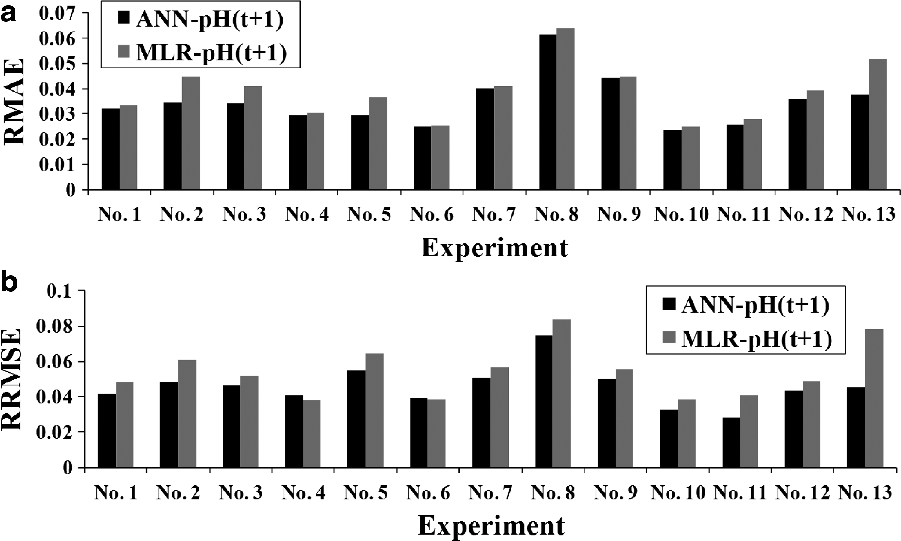
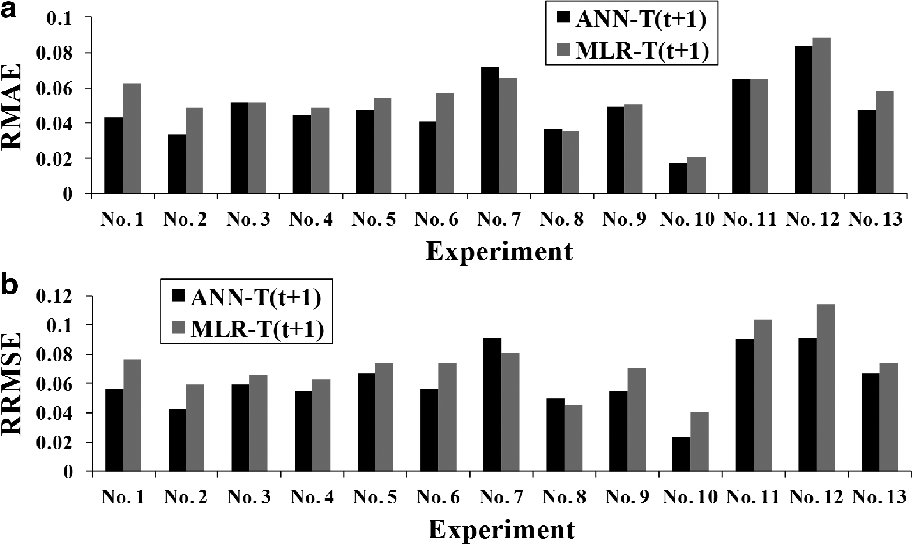
Scatter plots of observed versus predicted values obtained using the (a–c) ANN and (d–f) MLR models in 1- to 3-day-ahead T forecasts.

Figures 4 and 5 show the results of the 1-day-ahead forecast in each experiment obtained using the ANN and MLR models. In the case of pH, Fig. 4a shows that RMAE values were 0.024–0.062 in the ANN model and 0.025–0.064 in the MLR model, and Fig. 4b shows that RRMSE values were 0.028–0.074 in the ANN model and 0.038–0.083 in the MLR model. The average RMAE and RRMSE values of the two models were 0.037 and 0.049, and 0.04 and 0.056, respectively (Table 4). Similarly, in the case of temperature, the average RMAE and RRMSE values of the ANN and MLR models were 0.049 and 0.064, and 0.055 and 0.073, respectively (Table 5). These results demonstrate that the predictions obtained using the ANN models were more accurate than those obtained using the MLR models. This might be because neural networks perform favorably in applications when the functional form is nonlinear (Curram and Mingers, 1994).

FIG. 4.

(a) RMAE and (b) RRMSE values measured for ANN and MLR models in 1-day-ahead pH forecasts in each experiment conducted. RMAE, relative mean absolute error; RRMSE, relative root mean squared error.

FIG. 5.

(a) RMAE and (b) RRMSE values measured for ANN and MLR models in 1-day-ahead T forecasts in each experiment conducted.

Table 4.

RMAE, RRMSE, and COE Values Measured for ANN and MLR Models in 1- to 3-Day-Ahead pH Forecasts

	ANN-pH			MLR-pH
Δt-ahead forecast (day)	RMAE	RRMSE	COE	RMAE	RRMSE	COE
Δt = 1	0.037	0.049	0.954	0.040	0.056	0.941
Δt = 2	0.046	0.059	0.926	0.052	0.071	0.893
Δt = 3	0.053	0.076	0.864	0.064	0.088	0.820

ANN, artificial neural network; COE, coefficient of efficiency; MLR, multiple linear regression; RMAE, relative mean absolute error; RRMSE, relative root mean squared error.

Table 5.

RMAE, RRMSE, and COE Values Measured for ANN and MLR Models in 1- to 3-Day-Ahead T Forecasts

	ANN-T			MLR-T
Δt-ahead forecast (day)	RMAE	RRMSE	COE	RMAE	RRMSE	COE
Δt = 1	0.049	0.064	0.921	0.055	0.073	0.896
Δt = 2	0.062	0.081	0.879	0.077	0.101	0.813
Δt = 3	0.070	0.091	0.856	0.090	0.120	0.751

Tables 4 and 5 list the average skill scores of the 1- to 3-day-ahead pH forecast results obtained using the ANN and MLR models in terms of RMAE, RRMSE, and COE. The results obtained using the ANN-pH and MLR-pH models showed that with both models, the RMAE, RRMSE, and COE values were superior in the Δt = 1 forecasts than in the Δt = 2 and 3 forecasts. Furthermore, similar results were obtained in the temperature predictions. Thus prediction accuracy was high when the number of days was low.

Simulation and Comparison

Simulation process

As mentioned, two influential operational compost parameters were selected, pH and composting temperature, and thus two prediction models were constructed. To demonstrate the use of the two vital parameters, both temperature and pH were used to monitor the composting process. To simulate the real-time process, Fig. 6 illustrates the architecture of the real-time composting flowchart. The unit of computation interval is 1 day. A series of repetitive daily calculation steps are as follows:

Step 1: Start at time t = t₀;

Step 2: Receive eight parameters, denoted as dataset { A }_t (Table 2) from original compost at time t;

Step 3: Run the pH prediction model and the T prediction model by using the dataset { A } as inputs;

Step 4: Predict pH values of the L-d-ahead forecasts \documentclass{aastex}\usepackage{amsbsy}\usepackage{amsfonts}\usepackage{amssymb}\usepackage{bm}\usepackage{mathrsfs}\usepackage{pifont}\usepackage{stmaryrd}\usepackage{textcomp}\usepackage{portland, xspace}\usepackage{amsmath, amsxtra}\pagestyle{empty}\DeclareMathSizes{10}{9}{7}{6}\begin{document} $$\{ pH_{t + \Delta t}^{ \prime} , \Delta t \in [ 1 , L ] \} $$ \end{document} and T values of the L-d-ahead forecasts \documentclass{aastex}\usepackage{amsbsy}\usepackage{amsfonts}\usepackage{amssymb}\usepackage{bm}\usepackage{mathrsfs}\usepackage{pifont}\usepackage{stmaryrd}\usepackage{textcomp}\usepackage{portland, xspace}\usepackage{amsmath, amsxtra}\pagestyle{empty}\DeclareMathSizes{10}{9}{7}{6}\begin{document} $$\{ T_{t + \Delta t}^{ \prime} , \Delta t \in [ 1 , L ] \} $$ \end{document} ;

Step 5: Check whether \documentclass{aastex}\usepackage{amsbsy}\usepackage{amsfonts}\usepackage{amssymb}\usepackage{bm}\usepackage{mathrsfs}\usepackage{pifont}\usepackage{stmaryrd}\usepackage{textcomp}\usepackage{portland, xspace}\usepackage{amsmath, amsxtra}\pagestyle{empty}\DeclareMathSizes{10}{9}{7}{6}\begin{document} $$pH_{t + \Delta t}^{ \prime} < 8$$ \end{document} and \documentclass{aastex}\usepackage{amsbsy}\usepackage{amsfonts}\usepackage{amssymb}\usepackage{bm}\usepackage{mathrsfs}\usepackage{pifont}\usepackage{stmaryrd}\usepackage{textcomp}\usepackage{portland, xspace}\usepackage{amsmath, amsxtra}\pagestyle{empty}\DeclareMathSizes{10}{9}{7}{6}\begin{document} $$T_{t + \Delta t}^{ \prime}$$ \end{document} < 40°C. If yes, then record current time t_final = t+Δt and go to Step 6; otherwise, update time t = t + 1 and go to Step 7;

Step 6: Acquire compost product at time t_final derived from model prediction;

Step 7: Check whether t > d_max (where d_max is defined as maximal experimental days, set to 70 days). If yes, then the experiment is a failure, so go to Step 8; otherwise, repeat Steps 2–6;

Step 8: Stop at time t = t_final.

FIG. 6.

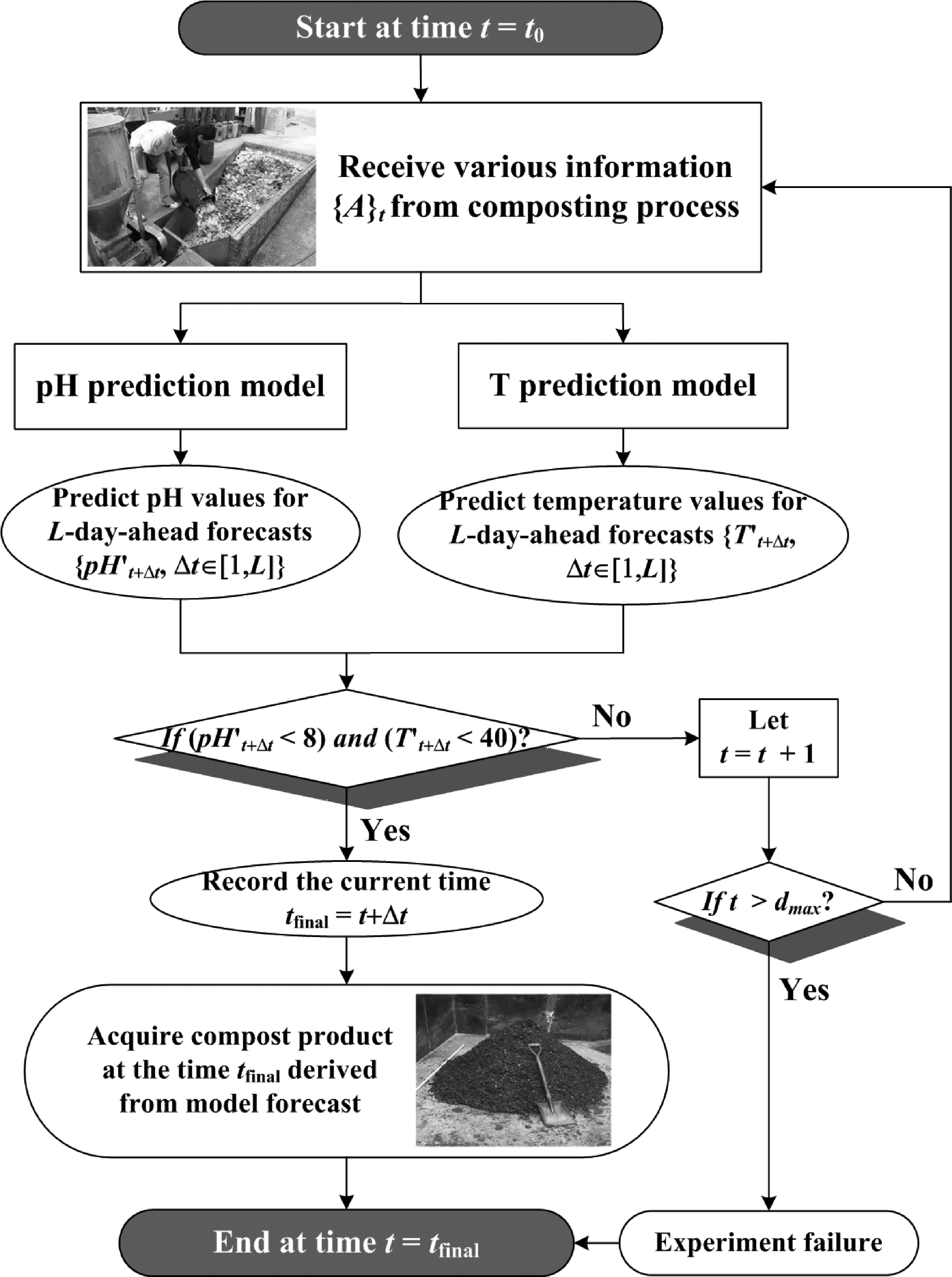
Architecture of composting real-time forecast process.

The criteria used for judging compost products are noted in Step 5; both temperature and pH were used to monitor the composting process and to evaluate the final mature product because of two reasons. According to the recommendations of Lin (2008), empirically, the composting process reached maturity and was ended at temperatures between 20 and 40°C in the experimental environment. Therefore, we assumed that 40°C could be used to stop modeling the composting process. Second, as mentioned in the preceding section, compost pH typically increases from 4.5–5.0 initially to 8.0–8.1 in the end product (Sundberg et al., 2004; Cekmecelioglu et al., 2005). Thus, we assumed that pH 8.0 will stop the composting process. In the following sections, we sequentially describe the models used for predicting pH and temperature.

Simulation results

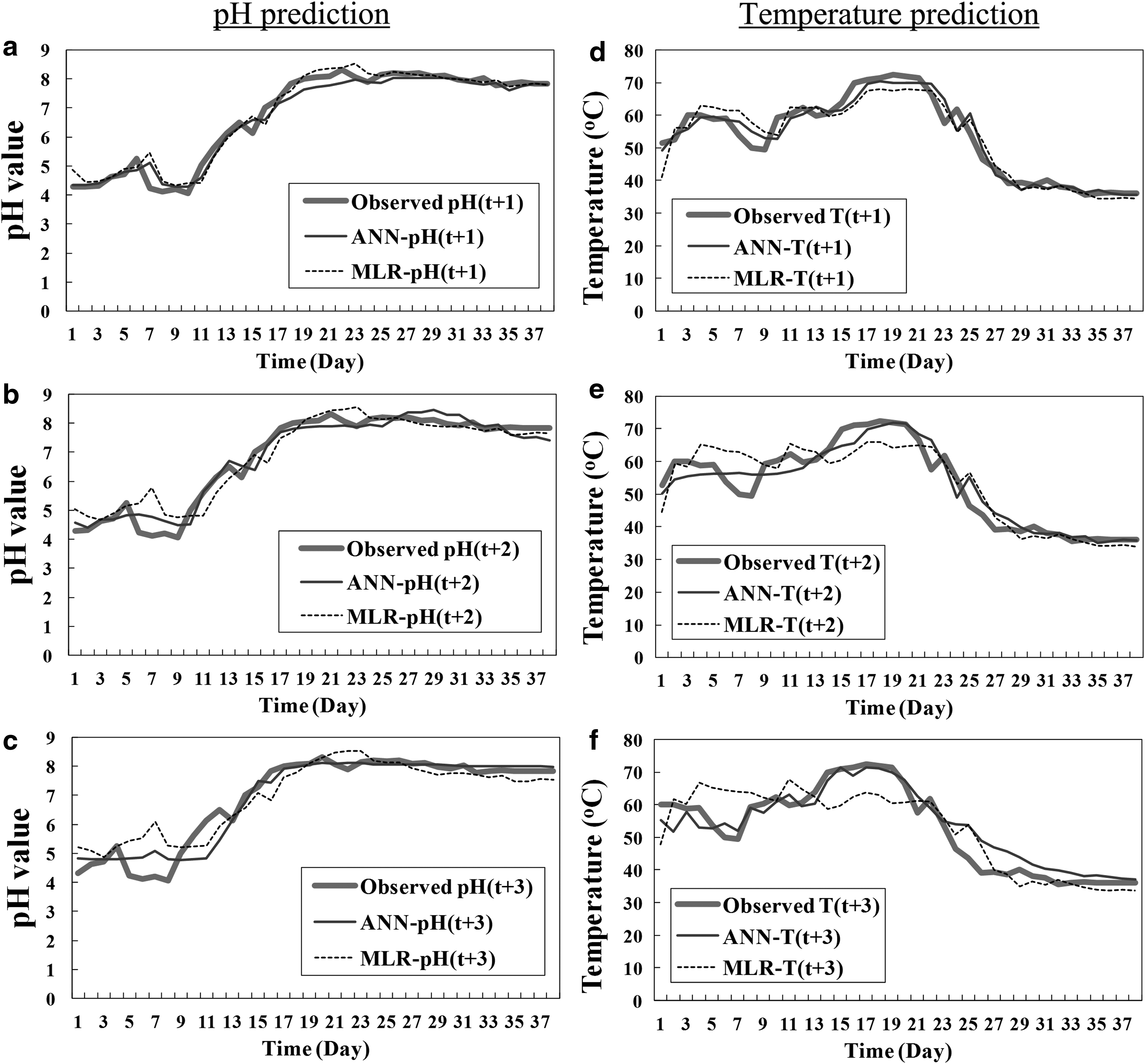
To evaluate the effectiveness of the presented methodology regarding the real-time forecast process of composting, two experiments (Nos. 1 and 12) were selected for simulation. The variations between the observed values and the predicted values obtained using the ANN- and MLR-based models of pH and temperature are plotted in Figs. 7 and 8.

FIG. 7.

Simulations of composting real-time forecast model in Experiment No. 1: (a–c) show 1- to 3-day-ahead predictions of pH; and (d–f) temperature predictions.

FIG. 8.

Simulations of composting real-time forecast process in Experiment No. 12: (a–c) show 1- to 3-day-ahead predictions of pH; and (d–f) temperature predictions.

Experiment No. 1

Variation of compost pH is shown in Fig. 7a−c. The observed records (Fig. 7a) show that the pH at t = 1 is 4.30 and that the pH reaches 8.31 on the 21st day before gradually decreasing to a steady value <8.0 on the 30th day. In the case of the ANN-pH and MLR-pH forecasts in Δt = 1, the pH values peak and then decrease slightly to a steady value <8.0 on the 30th and 29th days, respectively.

The variation of compost temperature is shown in Fig. 7d−f. The observed temperature records (Fig. 7d) show that T at t = 1 is 51.5°C and that fermentation temperature between 50 and 60°C is maintained from the start to the 13th day. Afterward, T increases rapidly, peaks at 72.4°C on the 18th day, and then gradually decreases to a steady value <40°C on the 31st day. In the case of the ANN-T and MLR-T forecasts in Δt = 1, the temperatures reach maximal values around 70°C and then decrease to T < 40°C on the 31st and 30th days, respectively.

Based on the proposed composting real-time forecast process (Fig. 6), we examined the conditions related to degree of degradation (i.e., “if ( \documentclass{aastex}\usepackage{amsbsy}\usepackage{amsfonts}\usepackage{amssymb}\usepackage{bm}\usepackage{mathrsfs}\usepackage{pifont}\usepackage{stmaryrd}\usepackage{textcomp}\usepackage{portland, xspace}\usepackage{amsmath, amsxtra}\pagestyle{empty}\DeclareMathSizes{10}{9}{7}{6}\begin{document} $$pH_{t + \Delta t}^{ \prime} < 8$$ \end{document} ) and ( \documentclass{aastex}\usepackage{amsbsy}\usepackage{amsfonts}\usepackage{amssymb}\usepackage{bm}\usepackage{mathrsfs}\usepackage{pifont}\usepackage{stmaryrd}\usepackage{textcomp}\usepackage{portland, xspace}\usepackage{amsmath, amsxtra}\pagestyle{empty}\DeclareMathSizes{10}{9}{7}{6}\begin{document} $$T_{t + \Delta t}^{ \prime} < 40$$ \end{document} )?”), and we determined that (1) the observed records showed that the mature product can be obtained on the 31st day; and (2) using the ANN- and MLR-based models on Δt = 1 day, the mature product was predicted to be obtained on the 31st and 30th days, respectively. Furthermore, in the case of Δt = 2 and 3, the mature compost product was predicted to be obtained, respectively, on the 31st and 29th days by using the ANN model, and on the 33rd and 28th days by using the MLR model. Thus, in this experiment, prediction accuracy was higher using the ANN model than using the MLR model.

Experiment No. 12

Figure 8 presents the variations of compost pH and temperature. The observed records show that pH and T at t = 1 are 4.55 and 46.30°C, respectively (Fig. 8a, d), after which they rise rapidly and peak at 8.31 and 72.6°C on the 11th and 8th days, respectively, and then gradually decrease to steady values <8.0 and <40°C on the 26th and 18th days, respectively. Therefore, the mature product can be obtained on the 26th day.

Using the ANN and MLR model forecasts in Δt = 1, the variations of compost pH and temperature show that under the mature composing conditions, the compost product is predicted on the 25th and 24th days, respectively (Fig. 8a, d). Moreover, in the case of Δt = 2, the mature product is predicted on the 25th day by using the ANN-based model and on the 27th day by using the MLR-based model; with Δt = 3, the mature compost product is predicted on the 23rd and 21st days by using the ANN- and MLR-based models, respectively.

All experiments

To assess the performance level of the composting real-time prediction based on all experiments, the absolute time error of degree of degradation (ET_dd) was defined and used to compute the average time of the absolute errors: \documentclass{aastex}\usepackage{amsbsy}\usepackage{amsfonts}\usepackage{amssymb}\usepackage{bm}\usepackage{mathrsfs}\usepackage{pifont}\usepackage{stmaryrd}\usepackage{textcomp}\usepackage{portland, xspace}\usepackage{amsmath, amsxtra}\pagestyle{empty}\DeclareMathSizes{10}{9}{7}{6}\begin{document} \begin{align*} { \rm ET} _ { \rm dd } = \frac { 1 } { m } \sum \limits_ { k = 1 } ^m \Big | T_k^ { est } - T_k^ { obs } \Big | \quad\quad\quad\quad (12) ,\end{align*} \end{document}

Where \documentclass{aastex}\usepackage{amsbsy}\usepackage{amsfonts}\usepackage{amssymb}\usepackage{bm}\usepackage{mathrsfs}\usepackage{pifont}\usepackage{stmaryrd}\usepackage{textcomp}\usepackage{portland, xspace}\usepackage{amsmath, amsxtra}\pagestyle{empty}\DeclareMathSizes{10}{9}{7}{6}\begin{document} $$T_k^{est}$$ \end{document} is the predicted arrival time of degree of degradation in Experiment No. k, \documentclass{aastex}\usepackage{amsbsy}\usepackage{amsfonts}\usepackage{amssymb}\usepackage{bm}\usepackage{mathrsfs}\usepackage{pifont}\usepackage{stmaryrd}\usepackage{textcomp}\usepackage{portland, xspace}\usepackage{amsmath, amsxtra}\pagestyle{empty}\DeclareMathSizes{10}{9}{7}{6}\begin{document} $$T_k^{obs}$$ \end{document} is the observed arrival time of degree of degradation in Experiment No. k, and m is the total number of experiments. Here, the smaller the ET_dd values, the more accurate the predictions.

Figure 9 illustrates the prediction performance levels of the ANN and MLR models in terms of the ET_dd measurements obtained using all experiments. In 1-day-ahead prediction, the ET_dd values are 0.67 and 1.22 days for the ANN and MLR models, respectively; these values calculated for the ANN model are also lower than those for the MLR model in 2- and 3-day-ahead predictions. Thus, the ANN model demonstrated accurate prediction ability. Comparison of the ET_dd values of the three lead times (Fig. 9) shows that the highest ET_dd values occur in 3-day-ahead predictions, which indicates that the uncertainty in predicting the time required for compost to mature increases with increasing lead times.

FIG. 9.

Average error rates of ANN- and MLR-based composting real-time forecast models.

Conclusions

Physical and chemical parameters affect the fermentation process. The information regarding these predicted parameters during the composting process can be referenced for design and operation of future composting plants. The findings of this study contribute toward the development of an effective and reliable prediction model for use in monitoring composting processes.

This work presents ANN- and MLR-based real-time composting forecast models that are developed to predict the influential operational compost parameters and to further simulate the time of the composting process. We conducted 13 experiments in an open-air facility on the campus of the National Kaohsiung Marine University, Taiwan. The composting mixtures comprised food waste, mature compost, sawdust, and soil, and both temperature and pH were measured to monitor the composting process and to evaluate the final product's maturity. Here, the prediction results are compared by using CC, RMAE, RRMSE, and COE values, and the results include the 1- to 3-day-ahead forecasts obtained using the two models. The pH and temperature predictions obtained using the ANN models have CC values of 0.979 and 0.956 in 1-day-ahead forecasts and greater slopes than the predictions obtained using the MLR models, which have CC values of 0.972 and 0.941. Similar results are obtained for 2- and 3-day-ahead forecasts. Thus, the ANN-model estimates are closer to the observed results than the estimates obtained using the MLR model. In terms of performance RMAE, RRMSE, and COE values, the results show that the pH and temperature predictions obtained using the ANN model are more accurate than those obtained using the MLR model in 1- to 3-day-ahead forecasts. In using ANN and MLR models to predict the maturity of food waste composts, the absolute time errors of degree of degradation are 0.67 and 1.22 days, respectively, in 1-day-ahead prediction, again indicating that prediction using ANN is more accurate than that using MLR.

The aforementioned results indicate that the methodology of the real-time composting forecast process developed in this study can be effectively used to predict composting time. Finally, the study's limitations and our suggestions for future studies are, for example, that the proposed methodology can be applied only in windrow systems; thus, complex in-vessel systems such as the negative-pressure aeration system could be studied in the future. Moreover, we used pH and temperature as indicators during the composting process. However, these indicators of maturity should be used carefully, because a stabilized temperature does not always indicate stabilized compost. This might suggest that the biological process slowed down, possibly because of a lack of moisture. Regarding the mixing ratios of the original compost, the materials are confined to percentage ranges. When a statistical data-driven model (such as ANN) is compelled by data, the model accuracy might decrease when the mixing ratio distinctly differs from the percentage ranges.

Footnotes

Acknowledgments

Support for this study under Grant No. MOST103-2111-M-464-001 provided by the Ministry of Science and Technology, Taiwan is greatly appreciated. The authors also acknowledge the constructive comments of the reviewers.

Author Disclosure Statement

No competing financial interests exist

References

Bach

P.D.

, Nakasaki

, Shoda

, and Kubota

(1987). Thermal balance in composting operations. J. Ferment. Technol., 65, 199.

Bishop

(1995). Neural Networks for Pattern Recognition. New York: Oxford University Press, p. 504.

Blaker

(2000). Minimax estimation in linear regression under restrictions. J. Stat. Plan. Inference., 90, 35.

Boniecki

, Dach

, Pilarski

, and Piekarska-Boniecka

(2012). Artificial neural networks for modeling ammonia emissions released from sewage sludge composting. Atmos. Environ., 57, 49.

Caputo

A.C.

, and Pelagagge

P.M.

(2002). RDF production plants: I. Design and costs. Appl. Therm. Eng., 22, 423.

Cekmecelioglu

, Demirci

, Graves

R.E.

, and Davitt

N.H.

(2005). Applicability of optimised in-vessel food waste composting for windrow systems. Biosyst. Eng., 91, 479.

Chang

Y.J.

, and Lin

M.D.

(2013). Compromising economic cost and air pollutant emissions of municipal solid waste management strategies by fuzzy multiobjective optimization model. J. Air Waste Manag. Assoc., 63, 712.

Chen

W.H.

, Lin

Y.C.

, Lin

J.H.

, Yang

P.M.

, and Jhang

S.R.

(2014). Treating odorous and nitrogenous compounds from waste composting by acidic chlorination followed by Alkaline sulfurization. Environ. Eng. Sci., 31, 583.

Curram

S.P.

, and Mingers

(1994). Neural networks, decision tree induction and discriminant analysis: An empirical comparison. J. Oper. Res. Soc., 45, 440.

10.

Déportes

, Benoit-Guyod

J.L.

, and Zmirou

(1995). Hazard to man and the environment posed by the use of urban waste compost: A review. Sci. Total Env., 172, 197.

11.

Diaz

L.F.

, Savage

G.M.

, Eggerth

L.L.

, and Golueke

C.G.

(1993). Composting and Recycling Municipal Solid Waste. Boca Raton, FL: Lewis Publishers, p. 121.

12.

Ekinci

, Keener

H.M.

, and Akbolat

(2006). Effects of feedstock, airflow rate, and recirculation ratio on performance of composting systems with air recirculation. Bioresour. Technol., 97, 922.

13.

Emmerling

, and Paulsh

(2001). Improvement of earthworm (Lumbricidae) community and activity in mine soils from open-cast coal mining by the application of different organic waste materials. Pedobiologia, 45, 395.

14.

Finger

S.M.

, Hatch

R.T.

, and Regan

T.M.

(1976). Aerobic microbial growth in semi-solid matrices: Heat and mass transfer limitations. Biotechnol. Bioeng., 18, 1193.

15.

Genell

, Nemes

, Steineck

, and Dickman

P.W.

(2010). Model selection in medical research: A simulation study comparing Bayesian model averaging and stepwise regression. BMC Med. Res. Methodol., 10, 108.

16.

Huang

G.H.

, Chi

G.F.

, and Li

Y.P.

(2005). Long-term planning of an integrated solid waste management system under uncertainty—II. A North American case study. Environ. Eng. Sci., 22, 835.

17.

Joshua

R.S.

, Macauley

B.J.

, and Mitchell

H.J.

(1998). Characterization of temperature and oxygen profiles in windrow processing systems. Compost. Sci. Util., 6, 15.

18.

Kaiser

(1996). Modelling composting as a microbial ecosystem: A simulation approach. Ecol. Model., 91, 25.

19.

Kim

J.D.

, Park

J.S.

, In

B.H.

, Kim

, and Namkoong

(2008). Evaluation of pilot-scale in-vessel composting for food waste treatment. J. Hazard. Mater., 154, 272.

20.

Kim

Y.S.

(2008). Comparison of the decision tree, artificial neural network, and linear regression methods based on the number and types of independent variables and sample size. Expert Syst. Appl., 34, 1227.

21.

Kishimoto

, Preechaphan

, Yoshida

, and Taguchi

(1987). Simulation of an aerobic composting of activated sludge using a statistical procedure. MIRCEN J. 3, 113.

22.

Kumar

, Ou

Y.L.

, and Lin

J.G.

(2010). Co-composting of green waste and food waste at low C/N ratio. Waste Manag. 30, 602.

23.

Liang

, Das

K.C.

, and McClendon

R.W.

(2003). The influence of temperature and moisture contents regimes on the aerobic microbial activity of a biosolids composting blend. Bioresour. Technol., 86, 131.

24.

Liang

, Leonard

J.J.

, Feddes

J.J.R.

, and McGill

W.B.

(2006). Influence of carbon and buffer amendment on ammonia volatilization in composting. Bioresour. Technol., 97, 748.

25.

Lin

(2008). A negative-pressure aeration system for composting food wastes. Bioresour. Technol., 99, 7651.

26.

Lin

, Wu

E.M.Y.

, Lee

C.N.

, and Kuo

S.L.

(2011). Multivariate statistical factor and cluster analyses for selecting food waste optimal recycling methods. Environ. Eng. Sci., 28, 349.

27.

Lin

, Sheu

D.S.

, Lin

T.C.

, Kao

C.M.

, and Grasso

(2012). Thermophilic biodegradation of diesel oil in food waste composting processes without bioaugmentation. Environ. Eng. Sci., 29, 117.

28.

Maier

H.R.

, and Dandy

G.C.

(1998). The effect of internal parameters and geometry on the performance of back-propagation neural networks: An empirical study. Environ. Model. Softw., 13, 193.

29.

Maliki

A.D.

, and Lai

K.M.

(2011). Design and application of a pre-composting test step to determine the effect of high fat food wastes on an industrial scale in-vessel composting system. Int. Biodeter. Biodegr., 65, 906.

30.

Mason

I.G.

(2006). Mathematical modelling of the composting process: A review. Waste Manag. 26, 3.

31.

McCartney

, and Tingley

(1998). Development of a rapid moisture content method for compost materials. Compost Sci. Util., 6, 14.

32.

Mohee

, White

, and Das

(1998). Simulation model for composting cellulosic (bagasse) substrates. Compost Sci. Util., 6, 82.

33.

Nakasaki

, Kato

, Akiyama

, and Kubota

(1987). A new composting model and assessment of optimum operation for effective drying of composting material. J. Ferment. Technol., 65, 441.

34.

Namkoong

, and Hwang

E.Y.

(1997). Operational parameters for composting night. Compost Sci. Util., 5, 46.

35.

Ndegwa

P.M.

, Thompson

S.A.

, and Merka

W.C.

(2000). A dynamic simulation model of in-situ composting of caged layer manure. Compost Sci. Util., 8, 190.

36.

Polprasert

(1996). Organic Waste Recycling: Technology and Management, 2nd ed. Chichester: Wiley, p. 69.

37.

Rantala

P.R.

, Vaajasaari

, Juvonen

, Schultz

, Joutti

, and Makela-Kurtto

(1999). Composting of forest industry wastewater sludges for agriculture use. Water Sci. Technol., 40, 187.

38.

Seki

(2000). Stochastic modeling of composting processes with batch operation by the Fokker–Planck equation. Trans. ASAE., 43, 169.

39.

Seo

J.Y.

, Heo

J.S.

, Kim

T.H.

, Joo

W.H.

, and Crohn

D.M.

(2004). Effect of vermiculite addition on compost produced from Korean food wastes. Waste Manag. 24, 981.

40.

Slater

R.A.

, and Frederickson

(2001). Composting municipal waste in the UK: Some lessons from Europe. Resour., Conserv. Recycling, 32, 359.

41.

Stombaugh

D.P.

, and Nokes

S.E.

(1996). Development of a biologically based aerobic composting simulation model. Trans. ASAE., 39, 239.

42.

Sundberg

, Smars

, and Jonsson

(2004). Low pH as an inhibiting factor in the transition from mesophilic to thermophilic phase in composting. Bioresour. Technol., 95, 145.

43.

Tai

H.S.

, and He

W.H.

(2007). A novel composting process for plant wastes in Taiwan military barracks. Resour. Conserv. Recycling., 51, 408.

44.

Wei

C.C.

(2012). Wavelet support vector machines for forecasting precipitations in tropical cyclones: Comparisons with GSVM, regressions, and numerical MM5 model. Weather Forecast. 27, 438.

45.

Wei

C.C.

(2013). Soft computing techniques in ensemble precipitation nowcast. Appl. Soft Comput., 13, 793.

46.

Wei

C.C.

, and Hsu

N.S.

(2008). Multireservoir flood-control optimization with neural-based linear channel level routing under tidal effects. Water Resour. Manag., 22, 1625.

47.

B.D.

, Huang

G.H.

, Zhang

G.J.

, Wei

Z.M.

, Qin

X.S.

, and Liu

H.L.

(2007). A temperature-guided three-stage inoculation method for municipal solid wastes composting. Environ. Eng. Sci., 24, 745.

48.

Zhang

, El-Mashad

H.M.

, Hartman

, Wang

, Liu

, Choate

, and Gamble

(2007). Characterization of food waste as feedstock for anaerobic digestion. Bioresour. Technol., 98, 929.

49.

Zhang

, Li

W.W.

, Zeng

G.M.

, Tang

, Feng

C.L.

, Huang

D.L.

, and Li

Y.P.

(2009). Novel neural network-based prediction model for quantifying hydroquinone in compost with biosensor measurements. Environ. Eng. Sci., 26, 1063.