Predicting Life Cycle Failures of On-Site Wastewater Treatment Systems Using Generalized Additive Models

Abstract

Poor performance of on-site wastewater treatment systems (OWTS) poses local and regional risks to public health and environmental quality. In the United States, local regulations control system design through permits issued at the time of installation. However, regulatory focus on one-time controls does not account for factors that influence performance after installation, notably asset management choices made by residential property owners. We develop a statistical method to predict performance over the OWTS life cycle to identify vulnerabilities and potential controls that reduce the risk of failure and contaminant release. A regression model based on Generalized Additive Models for location, scale and shape uses data from public records of reported OWTS failures, repairs and replacements, inspections, and assessed property values from Boulder County, Colorado, which has 14,300 OWTS. Severity of required system repairs and replacements over a 40-year period was associated with five factors: structural value, house square footage, number of required inspections, homeowner expenditures, and frequency of OWTS upgrades. Model results suggested that mandatory inspections through a mechanism such as renewable permits would significantly reduce life cycle repair/failure frequency and severity, lowering OWTS costs to owners and reducing public exposure to wastewater contaminants.

Introduction

In the United States, the array of strategies and technologies for wastewater collection, treatment, and discharge forms an organizational continuum from centralized publicly owned wastewater collection and treatment works (POTWs) to owner-operated on-site wastewater treatment systems (OWTS). POTWs treat wastewater flows from 10 to over 10⁶ m³/day and operate with discharge permits issued through the National Pollutant Discharge Elimination System (NPDES) that require regular monitoring and reporting of compliance. The capacity range of OWTS serving a family or small commercial enterprise is much narrower, with flows typically less than 8 m³/day (Crites and Tchobanoglous, 1998). Permits are typically issued by local agencies at the time of installation with no requirements for monitoring or reporting of performance unless the OWTS fails and triggers regulatory action.

POTWs and OWTS have a historical relationship. As the association of fecal waste with outbreaks of cholera and other water-borne diseases became known in the latter half of the nineteenth century, unregulated on-site systems for collection, passive treatment, and storage using privies, vaults, and cesspools were replaced by centralized sewer systems better able to handle increasing wastewater flows as residential piped water supply and use of flush toilets became widespread (Cosgrove, 1909; Burian et al., 2000). As a result, centralization and modernization of wastewater treatment have been linked, and while the technologies for on-site systems have improved, scientific knowledge, tradition, and prevailing public opinion lead many engineers, public health officials, policy makers, and the general public to favor centralized infrastructure over owner/user operated systems (EPA, 1997, 2002b; Burian et al., 2000; Etnier et al., 2005, 2007). Because of this history, OWTS may be inaccurately associated with isolated rural residences or considered a temporary solution to be replaced by centralized collection and treatment.

In fact, reliance on OWTS to provide a significant portion of global sanitation is growing especially in regions where no sanitation infrastructure exists. Currently, decentralized typically user-owned and maintained OWTS serve ∼25% of the population in the United States (EPA, 2003, 2008a), with over 25 million OWTS installed in suburban, high population density areas (EPA, 2008a). Due to continued land development outside existing collection system boundaries, limited treatment plant capacity, and the cost of new centralized wastewater infrastructure, ∼30% of new residential developments in the United States are constructed with septic systems (EPA, 1997, 2002a, 2002b, 2003). In 2005, it was estimated that OWTS served ∼26 million homes, many in urbanized communities, discharging four billion gallons of effluent per day (U.S. Census Bureau, 2006). The City of Los Angeles, for instance, has over 11,500 residential OWTS and many are located near impaired water bodies with elevated levels of nitrate and coliform indicator bacteria (“LA Sewers,” 2013).

However, unlike centralized facilities operating with NPDES permits, the performance of OWTS is not routinely documented, since monitoring of operations or discharged water quality is not required. The U.S. EPA estimates that 10% to 20% of OWTS in fact do not treat wastewater to acceptable levels (EPA, 2003) and some states estimate failure rates to be as high as 50% (EPA, 2002b). While one individual system failure may not pose a public health threat because the impacts are localized, the aggregate contaminant release from a cluster of poorly performing OWTS can have negative local and watershed-scale consequences. A survey of state water quality agencies ranked OWTS as the third greatest threat to groundwater quality, behind underground storage tanks and landfills (EPA, 1998).

Part of the challenge of ensuring OWTS functionality stems from their characteristic as impure public goods that have attributes of both common property resources associated with public goods, such as environmental quality and open access resources (OARs), which have undefined ownership and are often privatized. As an OAR, an OWTS creates externalities that generate public costs associated with environmental degradation or threats to public health (Turvey 1963; Hardin 1968). Without controls, the private responsibility of OWTS operation and maintenance required for the protection of the public resource, that is, the environment, creates an incentive to opt out of potentially costly maintenance activities, since opting in may offer no immediate benefit to the individual owner/user and opting out is seen as having a small and even undetected impact. Public Goods Theory implies that some regulation of the private right to use the environment as a waste sink is necessary to prevent the general degradation of environmental quality (Mohamed, 2009).

A comprehensive review of state-based OWTS regulations conducted by D'Amato et al. (2008) found that while most states regulate OWTS, regulations are by no means uniform. Furthermore, those states that have more extensive controls focus on installation, siting, and design factors contributing to OWTS failure, which have been widely studied. Existing OWTS performance models incorporate spatial, topographical, hydrologic, and other physical characteristics to identify locations where installing an OWTS may result in a high risk of failure (Hudson, 1986; Joubert et al., 2004; Cromer, 1999a, 1999b; Brown and Root Services, 2001; Kenway et al., 2001; Chen and Herr, 2002; McGuinness and Martens, 2003; Carroll et al., 2006; Oosting and Joy, 2011). However, a significant fraction of properly designed OWTS fail, indicating that technology-based design standards are not the only factors influencing system performance over what is presumed to be a very long life cycle on the order of 30 years or more (EPA, 2002b). OWTS may be designed and operated in a way that optimizes treatment performance and decreases both the frequency and resulting reparative costs of OWTS malfunctions, ultimately improving the overall system performance life (McKinley and Siegrist, 2011).

The premise of this research is that reliance on design-based standards is insufficient to insure OWTS performance over the system life and that the role of factors associated with system maintenance, owner knowledge, and usage must be considered. Moreover, as demand for use of increasingly sophisticated OWTS technologies for removal of nutrients or emerging trace contaminants grows, the number and complexity of owner-dependent operations will likely increase. Increasing dependence on OWTS as a global sanitation strategy underscores the need to understand how human/social variables such as organization, user motivation, and knowledge influence operation of OWTS. (Kaminsky and Javernick-Will, 2013).

Statistical modeling has been applied only recently to performance-based diagnostics of wastewater systems. Multivariate regression analysis using Generalized Linear Models (GLM) has been used to model treatment system response to water quality and wastewater variables (e.g., Weirich et al., 2011, 2015; Towler et al., 2013) adapting an approach used more widely in stochastic weather generation (e.g., Furrer and Katz, 2007; Kleiber et al., 2012, 2013; Verdin et al., 2015). Weirich et al. (2011) used GLM to predict the likelihood of POTW compliance with NPDES permit discharge limits using Discharge Monthly Report data in the U.S. EPA Integrated Compliance Information System (ICIS) (EPA, 2008b). Applying a similar inductive statistical approach to characterize OWTS performance would allow us to observe what practices, if any, differentiate well- and poor-performing OWTS based on the historical performance of real systems over a defined life.

Objectives

The objective of this study was to (1) identify user-associated factors that affect lifetime OWTS performance and (2) develop a predictive model to guide effective management of these systems by owners, environmental and public health agencies, and servicers.

Since no public data analogous to ICIS are available for on-site systems, the first component of this study is acquisition of data from OWTS permit and tax assessment records. In the absence of effluent quality data, information on costs associated with inspection, maintenance, repair, and replacement of OWTS components, which are public records, serves as a surrogate measure of poor performance. It should be noted that modeled outcomes based on this type of data also may provide highly communicable cost/benefit information to stakeholders, especially OWTS owners.

Because OWTS records are typically collected and maintained by county health departments; Boulder County Colorado was chosen as the site for data collection. The Boulder County Public Health Department oversees permits for 14,300 OWTS and also conducts comprehensive permit and public education programs (“SepticSmart Program,” 2015). Variables generated from collected data are then subjected to a regression modeling approach, Generalized Additive Models for Location, Scale and Shape (GAMLSS) (Rigby and Stasinopoulos, 2005) to select the postinstallation factors associated with the level of OWTS performance over the system's expected life. The predictive model will enable regulators to define actionable management guidelines for postinstallation practices that can be incorporated into county or state regulations to improve OWTS reliability and save owners the costs of catastrophic failure. In addition, the model will provide a means to communicate wastewater management alternatives and associated financial trade-offs to communities in a quantifiable and comparable way.

Methods

The methods of this study are discussed in the three following sections: (1) data collection; (2) selection of the performance indicator and ten user-associated independent variables; and (3) development of the GAMLSS method for simulation of OWTS performance.

Data collection

The Boulder County OWTS study site is located in the Boulder Creek-St. Vrain Creek watershed in northeastern Colorado, encompassing an area of ∼190,000 hectares and 300,000 residents (U.S. Census Bureau, 2015). There are over 14,300 OWTS in the County serving ∼50,000 residents as well as 21 POTWs with a total capacity of 110,000 m³/d serving the rest of the population (BCPH, 2013; EPA, 2008b). Estimated flow from the 14,300 OWTS is ∼27,000 m³/d, based on a residential flow of 2 m³/d (EPA, 1980). OWTS are located in a highly variable terrain, including mountain communities at elevations exceeding 2,600 m and residents on the eastern plans at 1,600 m. Approximately, two-thirds of the OWTS for which the County has any records received permits at the time of installation.

The OWTS sample consisted of failed or poorly functioning systems selected by searching the database of repair permits maintained by the Boulder County Public Health (BCPH) Department. Repair permits were screened to select for OWTS having conditions associated with visible failures such as wastewater surfacing, odor or mechanical malfunctions resulting in system repairs, and replacement or reported functional breakdown. The search returned 215 properties with reported OWTS failures from 2003 to 2013. While the permit database contains applications dating back over 50 years, records of specific reasons for permits did not begin until 2003, limiting the documented failures to after 2003 repair permits. That said, many of the early repair permits available documented visible failures, but the evidence exists in the form of hand written notes on the permit applications and therefore was not searchable in the database. From 215 OWTS in the original sample, only systems that had a County-approved inspection at the time of installation were selected for analysis. This reduced the number of properties in the sample from 215 to 120. Using only permitted sites provides a control for siting and design criteria set by the County. The fact that over half the failed systems in the County met initial design and siting standards supports the premise of this study that design standards are not sufficient to ensure performance.

The selected OWTS sample is distributed throughout the County area (Fig. 1) and captures variability in neighborhood/community affluence, housing density, and distance to professional OWTS servicers. The breadth of geographic and demographic attributes of the sample is selected to enable the application of results in other communities/regions.

FIG. 1.

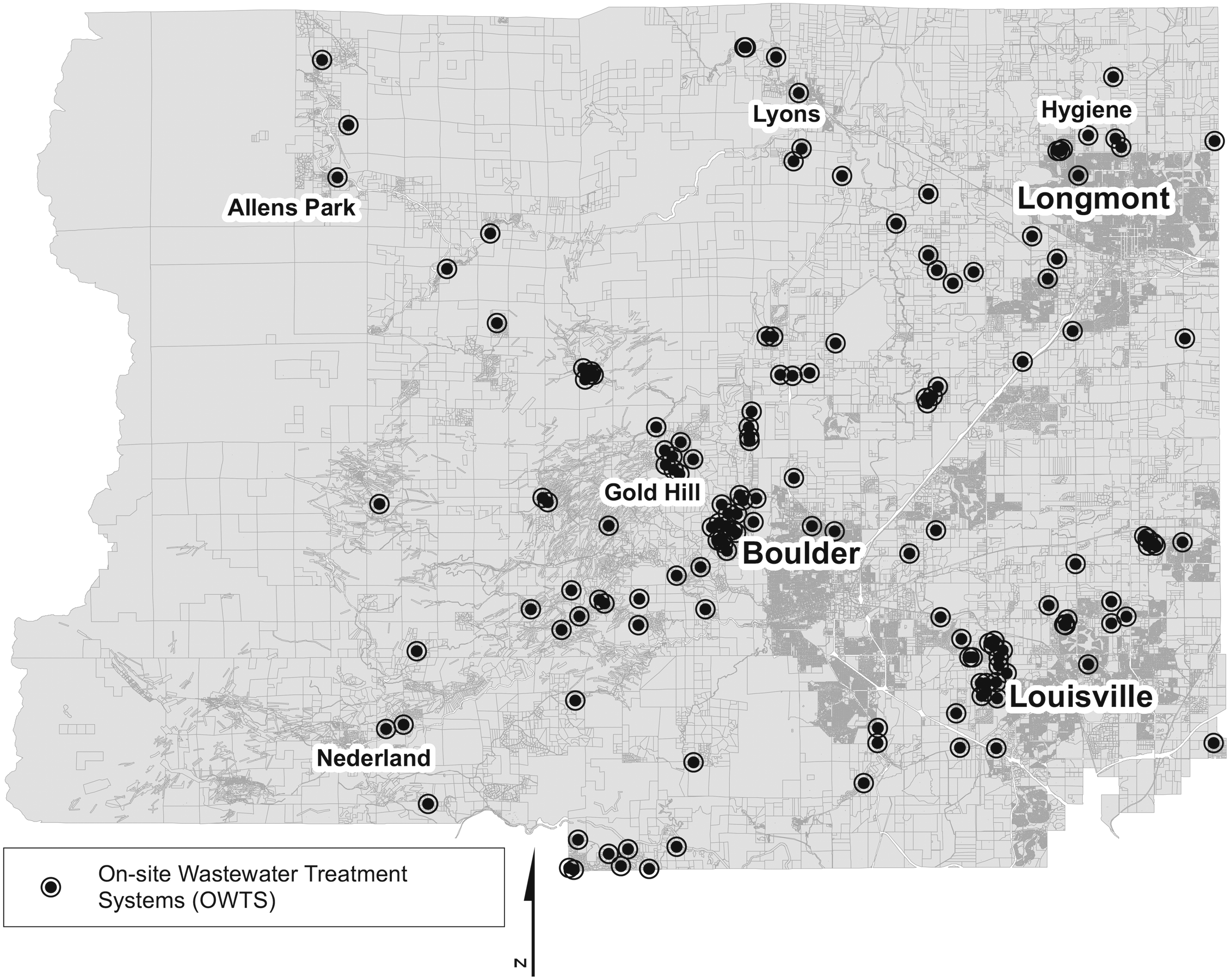
Geographic distribution of sampled on-site wastewater treatment systems (OWTS) repair permits in Boulder County, Colorado (Boulder County Public Health, 2013).

Information in the repair permit applications for each of the 120 OWTS, primarily scanned hand-written originals, was coded to define a failure measure and quantified attributes of the properties and the owners' operation and maintenance history.

Variable definition

Dependent variable

Failure has been generally defined as not meeting some designated performance standard (Etnier et al., 2005). However, there is no recognized definition of OWTS failure. Failure has been commonly used in the OWTS industry and in the literature to specify major operational faults described above and loss of equipment integrity, such as cracking of septic tanks and/or piping. For this study, the failure measure for each OWTS is the sum of the estimated cost of all repairs requiring a permit, annualized to a 40-year period of record from 1973 to 2013. Thus, failure incorporates both the frequency of major repairs and their magnitude, producing the dependent variable (Y) of annual repair severity expressed in U.S. dollars.

Repairs were classified into minor, moderate, and major, using cost estimates provided by BCPH staff, as described in the next section. The 40-year life cycle was selected based on the average length of time between the installation inspection and the date of the most recent repair permit.

For this study, a minor repair, defined by BCPH, is any repair to the septic tank or pipes. Moderate repairs refer to extraordinary maintenance or replacement of the soil treatment unit (STU). Failure of both the septic tank and STU constitutes a major repair often requiring replacement of all OWTS components.

The cost estimates for minor, moderate, and major repairs are based on the results of an informal survey of OWTS installers and servicers conducted by the BCPH over 10 years ago. Due to property slope, size, water table levels, soil substrate, and location, the cost of any type of repair can vary widely. For example, the BCPH estimated cost of a moderate repair of the STU ranged from $4,860 to $21,800. However, the estimates provide relative benchmarks for minor, moderate, and major repair costs adequate for modeling the severity distribution, which can be updated as new cost information is available. The average of the range of estimated repair costs for each category was as follows: minor, $3,066; moderate, $9,173; and major, $14,866. The repair cost does not include the cost of the repair permit, which is uniform for all repairs, or the cost to hire an engineer for more significant restorations. Engineering costs were excluded from this study because they vary greatly based on attributes associated with the system's location and design complexity. While this information affects the total cost of repair, the infrastructure and labor costs of each repair type included in our analyses differentiate between the types of failures and their relative severity.

Figure 2 shows the sample distribution of the annualized repair severity variable as a histogram along with admissible probability density functions, which will be further discussed in the OWTS Repair Severity Model section. The data appear to be categorical in nature, even though cost of repair is a continuous variable. Approximately, 60% of the sample has a repair severity value estimated to be $372 per year.

FIG. 2.

Distribution of OWTS annual repair severity data measured as cost (USD) compared to the Weibull and gamma regressions for the 120 OWTS in the sample.

Independent variables

Using information from the Boulder County Assessor's property tax database, property inspection documents, and repair/replacement applications, ten independent variables were defined, which map to six categories that previous researchers have related to long-term OWTS performance (Kaminsky and Javernick-Will, 2013). The categories are technical, referred to herein as physical status (PHYS); organizational (ORG), related to the degree of community or institutional control; economic status of owner (ECON); owner knowledge of system operation (KNOW); user motivation (UM), related to interests affecting owner choices; and other (OTHER). The ten variables related to these categories are described in Table 1. The independent variable values for each OWTS for the 40-year period from 1973 to 2013 are coded and stored with the associated annual repair severity values and unique land parcel ID for each OWTS site.

Table 1.

Independent Variables Hypothesized to Influence OWTS Performance with Definitions, Sources, and Category Type

Variable	Symbol	Variable definition	Relation to variable	Category
Property transfer inspections	PT	The number of property transfers after 2008 with documented inspections.	The Property Transfer Regulation effective since 2008 states that before property sale or title transfer, the owners of the dwelling have to obtain a certified inspection and disclose any system issues to the buyer. The value represents the frequency of regulated system inspection.	ORG
Property sales (after 2008)	PS	Total number of times a property changed ownership after 2008		UM/KNOW
Property sales (before 2008)	EPS	Frequency of title transfers and sales between 1973 and 2008		UM/KNOW
Loan inspections	LI	Total number of documented OWTS inspections that occurred as a result of a loan application.	Before 2008, Boulder County recorded nonmandatory OWTS inspections recommended by some mortgage lenders, such as USDA, VA, and FHA, with further tests and repairs if problems were found.	ORG
Water supply	WS	0 = private water supply (i.e., wells and cisterns)1 = public water supply (i.e., supplied by municipality or water district)	Availability of private water supplies may be associated with greater demand and OWTS loading (Nauges and Van den Berg, 2006). OWTS owners with private wells may be more likely to protect their water source.	UM/OTHER
Structural value	SV	Assessed value of structure, excluding land value, in USD	The structural value of the house is used as a proxy for income and ability to pay for repairs and maintenance (Nieswiadomy and Molina, 1989).	ECON
Living area	LA	Living area in square feet	Statistically, larger homes consume more water, increasing the wastewater load to the system (Mayer and DeOreo, 1999).	ECON/TECH
Change in bedroom count	RC	The difference between the number of bedrooms when the permit was issued and at the time of the last repair	The number of bedrooms is considered to be associated with OWTS loading and typically is used to specify OWTS sizing.	TECH
Change in bathroom count	BC	The difference between the number of bathrooms when the permit was issued and at the time of the last repair	Number of bathrooms is a greater factor in OWTS loading than the number of bedrooms, although two are often related.	TECH
Upgrades	UP	Cost of OWTS upgrades resulting from added bedrooms	Upgrades can be systems retrofitted to accommodate increased hydraulic loading.	OTHER

OWTS repair severity model

We used a variation of the Generalized Linear Model (GLM) regression method to evaluate the relationship between the annual repair severity of the sample OWTS population and the independent variables in Table 1. The application of the identified relationships is then used to predict the estimated annual repair severity of the larger OWTS population (Dowdy et al., 2004).

The GLM provides a more flexible approach to regression than a standard linear regression model. In the GLM, the response variable, Y, is assumed to be a realization from any distribution in the exponential family. \documentclass{aastex}\usepackage{amsbsy}\usepackage{amsfonts}\usepackage{amssymb}\usepackage{bm}\usepackage{mathrsfs}\usepackage{pifont}\usepackage{stmaryrd}\usepackage{textcomp}\usepackage{portland, xspace}\usepackage{amsmath, amsxtra}\pagestyle{empty}\DeclareMathSizes{10}{9}{7}{6}\begin{document} \begin{align*}Y \,\sim \,( G ) ({\theta}) \tag{1}\end{align*} \end{document}

where G(.) is any exponential type distribution and θ is the set of parameters that define G. A link function, η, relates the expected value of θ and consequently that of Y( θ ), as a linear function of independent variables or covariates X , as follows: \documentclass{aastex}\usepackage{amsbsy}\usepackage{amsfonts}\usepackage{amssymb}\usepackage{bm}\usepackage{mathrsfs}\usepackage{pifont}\usepackage{stmaryrd}\usepackage{textcomp}\usepackage{portland, xspace}\usepackage{amsmath, amsxtra}\pagestyle{empty}\DeclareMathSizes{10}{9}{7}{6}\begin{document} \begin{align*}\eta ( E ( \bold\theta ) ) = \textbf{\textit{X}} { \bold\beta}^T \tag{2}\end{align*} \end{document}

where η(.) is the link function, β ^T is the vector of model parameters and X is the set of covariates. The residuals are defined as follows: \documentclass{aastex}\usepackage{amsbsy}\usepackage{amsfonts}\usepackage{amssymb}\usepackage{bm}\usepackage{mathrsfs}\usepackage{pifont}\usepackage{stmaryrd}\usepackage{textcomp}\usepackage{portland, xspace}\usepackage{amsmath, amsxtra}\pagestyle{empty}\DeclareMathSizes{10}{9}{7}{6}\begin{document} \begin{align*}\varepsilon = Y - E \;( Y ) \tag{3}\end{align*} \end{document}

They are assumed to be normally distributed and uncorrelated as with a standard linear regression (McCullagh and Nelder, 1989). E(Y) is the expected value of Y determined from the model.

Standard linear models require Y to be from a normal distribution. Consequently, to model variables that are non-negative, positively skewed, discrete, or binary violates the normality assumption and thus cannot be readily modeled using a standard linear model. Assuming a binomial distribution for the response variable reduces the GLM to a logistic regression; a Poisson distribution makes it a Poisson regression model and so on (McCullagh and Nelder, 1989). Of course, a normal distribution assumption reduces this to a standard linear regression. The ability to model a variety of distributions in the exponential family is the major advantage of GLM (McCullagh and Nelder, 1989). Replacing G(.) with an extreme value distribution allows this approach to model extremes as shown in the modeling of extremes in water turbidity by Towler et al. (2013).

Since every OWTS in the sample was repaired at least once, the response variable Y for all 120 systems is greater than zero and a positively skewed distribution—as displayed in Fig. 2. The gamma distribution has been used in a GLM of POTW compliance data that also are positively skewed (Weirich et al., 2011). However, the OWTS data have long tails due to members of the sample with extremely high or low values of repair severity, and the Weibull distribution is better suited to capture tail behavior compared to the gamma distribution (e.g., Katz et al., 2002). While GLM provides computational flexibility, the assumption that the dependent variable Y must be represented by a distribution in the exponential family restricts its ability to model data using, for example, a Weibull distribution, which is not part of this family. Furthermore, the GLM framework is largely for modeling a single parameter of the distribution with a link function. To overcome this limitation, Rigby and Stasinopoulos (2001; 2005) and Akantziliotou et al. (2002) introduced generalized additive models for location, scale, and shape (GAMLSS). GAMLSS relax the exponential family distribution constraint for the response variable and allow a larger distribution family, including those with long tails such as Weibull. Furthermore, it can admit additive functions of the independent variable that can be linear or nonlinear, providing more flexibility in modeling.

Like GLM, for GAMLSS, a smooth link function, g_k(.), transforms the expectation of each parameter in the representative Y distribution, \documentclass{aastex}\usepackage{amsbsy}\usepackage{amsfonts}\usepackage{amssymb}\usepackage{bm}\usepackage{mathrsfs}\usepackage{pifont}\usepackage{stmaryrd}\usepackage{textcomp}\usepackage{portland, xspace}\usepackage{amsmath, amsxtra}\pagestyle{empty}\DeclareMathSizes{10}{9}{7}{6}\begin{document} $$f ( y_i \mid \theta^i )$$ \end{document} , to a set of predictors. The probability distribution function is conditional on θⁱ, where \documentclass{aastex}\usepackage{amsbsy}\usepackage{amsfonts}\usepackage{amssymb}\usepackage{bm}\usepackage{mathrsfs}\usepackage{pifont}\usepackage{stmaryrd}\usepackage{textcomp}\usepackage{portland, xspace}\usepackage{amsmath, amsxtra}\pagestyle{empty}\DeclareMathSizes{10}{9}{7}{6}\begin{document} $$\theta^i = ( \theta_{i1} , \theta_{i2} , \ldots , \theta_{ik} )$$ \end{document} is a vector of k parameters, where k depends on the distribution type. \documentclass{aastex}\usepackage{amsbsy}\usepackage{amsfonts}\usepackage{amssymb}\usepackage{bm}\usepackage{mathrsfs}\usepackage{pifont}\usepackage{stmaryrd}\usepackage{textcomp}\usepackage{portland, xspace}\usepackage{amsmath, amsxtra}\pagestyle{empty}\DeclareMathSizes{10}{9}{7}{6}\begin{document} \begin{align*}g_k ( \theta_{ik} ) = \eta_k = \textbf{\textit{X}}_k \beta_k + \sum \limits^{J_{k}}_{j = 1} h_{jk} x_{jk} \tag{4}\end{align*} \end{document}

Each parameter, θ_ik, is related to the set of explanatory variables, X _k, and a parametric vector, β _k. The term \documentclass{aastex}\usepackage{amsbsy}\usepackage{amsfonts}\usepackage{amssymb}\usepackage{bm}\usepackage{mathrsfs}\usepackage{pifont}\usepackage{stmaryrd}\usepackage{textcomp}\usepackage{portland, xspace}\usepackage{amsmath, amsxtra}\pagestyle{empty}\DeclareMathSizes{10}{9}{7}{6}\begin{document} $$\sum \nolimits^{J_{k}}_{j = 1} h_{jk}x_{jk}$$ \end{document} represents the random component and can be either a semiparametric or nonparametric additive model (Rigby and Stasinopoulos, 2005).

To determine the impact of user operations on the expected annual repair severity of OWTS over a 40-year period, all independent variables and variable interactions were incorporated in the GAMLSS using the GAMLSS package in the open-source statistical program R (www.r.project.org), and all combinations of variables were tested to determine the distribution parameters, θⁱ, using the Akaike Information Criteria (AIC, Akaike, 1974). AIC select a best model by considering all the possible subsets of the independent variables from the fit model. For each model, the generalized Akaike Information Criteria (GAIC), specific to GAMLSS, are calculated as follows: \documentclass{aastex}\usepackage{amsbsy}\usepackage{amsfonts}\usepackage{amssymb}\usepackage{bm}\usepackage{mathrsfs}\usepackage{pifont}\usepackage{stmaryrd}\usepackage{textcomp}\usepackage{portland, xspace}\usepackage{amsmath, amsxtra}\pagestyle{empty}\DeclareMathSizes{10}{9}{7}{6}\begin{document} \begin{align*}GAIC = - 2 \hat\ell ( \theta ) + ( N * k ) \tag{5}\end{align*} \end{document}

where \documentclass{aastex}\usepackage{amsbsy}\usepackage{amsfonts}\usepackage{amssymb}\usepackage{bm}\usepackage{mathrsfs}\usepackage{pifont}\usepackage{stmaryrd}\usepackage{textcomp}\usepackage{portland, xspace}\usepackage{amsmath, amsxtra}\pagestyle{empty}\DeclareMathSizes{10}{9}{7}{6}\begin{document} $$\hat\ell ( \theta )$$ \end{document} is the logarithm of the model likelihood function reflecting the subset of explanatory variables that are obtained from the iterated weighted least squares method (IWLS), N is the penalty for additional parameters, which has a default value of 2, typical for AIC, and k is the number of model parameters. The model with the lowest GAIC is selected as the ‘best model’ (Stasinopoulous et al., 2008).

Cross-validation

To evaluate the model performance on an independent data set, a random number of observations, ∼15% of the total data set or about 18 points, are dropped. The model is fitted to the remaining ∼85% of the data and used to predict the dropped values, and performance measures such as R² (square of the correlation coefficient between the observed and model predicted values) and RMSE (root mean squared error) are computed. This is repeated a thousand times, and the measures are displayed as boxplots to provide insights into the variability of the model skill.

Sensitivity analysis

The range of cost estimates for minor, moderate, and major repairs motivated us to consider the sensitivity of the Weibull model to changing costs. Because the BCPH cost estimates are over 10 years old, the possibility of underestimating the annual repair severity is the greater concern. Therefore, the sensitivity analysis consists of generating two new models using the following repair cost conditions. Model II: sensitivity to the cost of major repairs only by retaining the average cost for the minor and moderate repairs used in the original model (Model I), but increasing the cost for the major repairs to the high value of the range; Model III: increasing the cost of repairs for all repair categories to the high value in the range.

Results

A GAMLSS belonging to the Weibull distribution family was fit to the dependent variables and annual repair severity data, using the log link function. The GAMLSS of repair severity is represented as follows: \documentclass{aastex}\usepackage{amsbsy}\usepackage{amsfonts}\usepackage{amssymb}\usepackage{bm}\usepackage{mathrsfs}\usepackage{pifont}\usepackage{stmaryrd}\usepackage{textcomp}\usepackage{portland, xspace}\usepackage{amsmath, amsxtra}\pagestyle{empty}\DeclareMathSizes{10}{9}{7}{6}\begin{document} \begin{align*}Y \,\sim\, WEI ( \mu , \sigma ) \tag{6}\end{align*} \end{document}

where Y is the response variable, annual repair severity, and μ and σ are the scale and shape parameters, respectively, of the Weibull distribution (WEI). The best model of the scale and shape parameters based on GAIC resulted in the following expressions. \documentclass{aastex}\usepackage{amsbsy}\usepackage{amsfonts}\usepackage{amssymb}\usepackage{bm}\usepackage{mathrsfs}\usepackage{pifont}\usepackage{stmaryrd}\usepackage{textcomp}\usepackage{portland, xspace}\usepackage{amsmath, amsxtra}\pagestyle{empty}\DeclareMathSizes{10}{9}{7}{6}\begin{document} \begin{align*} \begin{split} log \ E ( \mu ) & = 5.96+ 7.54e - 8 * SV + 2.96e - 5 \ \\& * LA - 0.05 * UP - 1.4 * PT - 0.10 \ \\& * PS - 1.21 * ( UP * PT ) - 0.001 \ \\& * ( SV * PT ) - 1.40e - 6 * ( SV * PT ) \\& - 1.64 * ( PT * PS )\end{split} \tag{7}\end{align*} \end{document} \documentclass{aastex}\usepackage{amsbsy}\usepackage{amsfonts}\usepackage{amssymb}\usepackage{bm}\usepackage{mathrsfs}\usepackage{pifont}\usepackage{stmaryrd}\usepackage{textcomp}\usepackage{portland, xspace}\usepackage{amsmath, amsxtra}\pagestyle{empty}\DeclareMathSizes{10}{9}{7}{6}\begin{document} \begin{align*}log \ E ( \sigma ) = 1.023 \tag{8}\end{align*} \end{document}

Equations (6) and (7) indicate that OWTS performance is related to five of the ten individual independent variables and four combinations of the variables. The individual factors selected are the assessed structural value of the home (SV), square footage of the home (LA)—both are considered proxies for household affluence or ability to pay, the number of complete required system inspections (PT) as a result of the 2008 Boulder County Property Transfer regulation for OWTS, the total number sales after 2008 where a property transfer inspection was not documented (PS), and the frequency and cost of OWTS upgrades resulting from adding a bedroom (UP).

The expected value of the shape parameter E(σ) is a constant estimated by fitting a Weibull distribution to the observed data. It is common in these models with a smaller number of data that, such as the case here, the GAIC keep the shape parameter constant, as varying the shape parameter can make the model fit highly variable and the results difficult to interpret. The nonlinear combination of the five variables describing both the scale and shape parameters creates the Weibull distribution for each observation; therefore, each OWTS observation has a unique scale with a constant shape.

The Analysis of Variance (ANOVA) table (model I in Table 2) shows the significance of each variable in the model based on its p-value. The significance threshold was set at 0.1 (i.e., 90% confidence) for this study. The four combined variables, UP*PT, LA*PT, SV*PT, and PT*PS, are significant at greater than 90% confidence. Of the individual variables, only the number of property transfers after 2008 when a full inspection was required met the significance criterion. While not all of the individual variables are significant at 90% confidence or higher (i.e., p-value <0.01) in the best model, the best model from GAIC or other such criteria selects the group of variables that jointly improve the estimation of annual repair severity. However, the variables that are not significant tend to have coefficient values close to zero. With one exception, an increase in the value of individual and combined factors, including the variable number of required inspections after 2008, PT, was associated with a decrease in annual repair severity, as reported under Model I in Table 2, column 2.

Table 2.

Reliability Model (Model 1) ANOVA Table and Model Sensitivity to Repair Cost Estimates

GAIC	Model I 1533.79				Model II 1769.30		Model III 1766.75
Covariate	Influence	Estimate	Std. error	P-value	Estimate	P-value	Estimate	P-value
μ coefficients
(Intercept)	+	5.96	0.09	<0.001	6.62	<0.001	6.85	<0.001
RC		—	—	—	0.13	0.082	—	—
SV	+	7.54e-7	3.23e-7	0.82	4.99e-7	0.197	—	—
LA	+	2.96e-5	5.02e-5	0.56	—	—	—	—
UP	−	0.05	0.08	0.53	0.38	0.122	−0.05346	0.59
PT	−	1.4	0.42	0.001	−0.32	0.054	−0.36371	0.02
PS	−	0.10	0.08	0.20	−0.12	0.336	−0.06832	0.47
UP^*PT	−	1.21	0.40	0.003	−1.99	<0.001	−1.84926	0.003
PT^*PS	−	1.64	0.44	<0.001	−2.00	<0.001	−1.83440	<0.001
LA^*PT	−	0.001	2.08e-4	<0.001	—	—	—	—
SV^*UP		—	—	—	−2.60e-6	0.001	—	—
UP^*PS		—	—	—	0.37	0.091	—	—
SV^*PT	+	1.40e-6	3.16e-6	<0.001	—	—	—	—
σ coefficients
(Intercept)		1.023	0.07	<0.001	0.776	<0.001	0.853	<0.001

Shaded entries are the variables that are consistently associated with repair severity in all three scenarios.

GAIC, generalized Akaike Information Criteria.

Model diagnostics

The GAMLSS [Eqs. (6) and (7)] provide the best estimate of the two parameters of the Weibull distribution describing the repair severity for each observation as a function of the selected independent variables. Consequently, the median and the 95% confidence intervals can be obtained from the estimated sample distribution. While a predictive model encompassing both extreme and the median results would be ideal, the primary concern is whether the model is a good predictor of annual repair severity for the average OWTS. Average system performance as reflected by the expected annual repair severity over the system's life is a potential decision factor for homeowners and can aid community and regional planning and management decisions when comparison of the costs of on-site and centralized systems is desirable.

The observed values and the predicted annual repair severity costs have an R² of 0.406, indicating that the model captures ∼40% of the overall variability. R² values less than 50% are acceptable in behavioral and social science fields, where typically the percentage of variance accounted for is smaller given the inherent variability of human nature (Hunter and Schmidt, 2004). Furthermore, even with a low R² value, the presence of statistically significant predictors still allows important conclusions to be drawn about how variations in the predictor values are associated with changes in the annual repair severity.

Figure 3 shows the annual repair severity in dollars for each system in the sample compared to the model expected value and 95% confidence interval. The figure shows that the model underpredicts the extremes and predicts well near the central values for annual repair severity. This suggests that there are additional variables that potentially contribute to the likelihood of highly performing systems—those requiring few repairs—and systems requiring frequent and costly major repairs that are ultimately more vulnerable to failure. The confidence intervals (Fig. 3) are asymmetric and shifted in the same direction as the repair severity, suggesting that they are able to capture the variability well—unlike traditional regression approaches, which provide symmetric intervals. Figure 4 shows the observed and modeled values for annual repair severity as boxplots, as a function of the significant and highly influential variable, of a number of property transfers after 2008 with required inspections (PT). No property had more than one required inspection after 2008; however, even one inspection had a clear beneficial impact on annual repair severity, as captured in the Weibull regression.

FIG. 3.

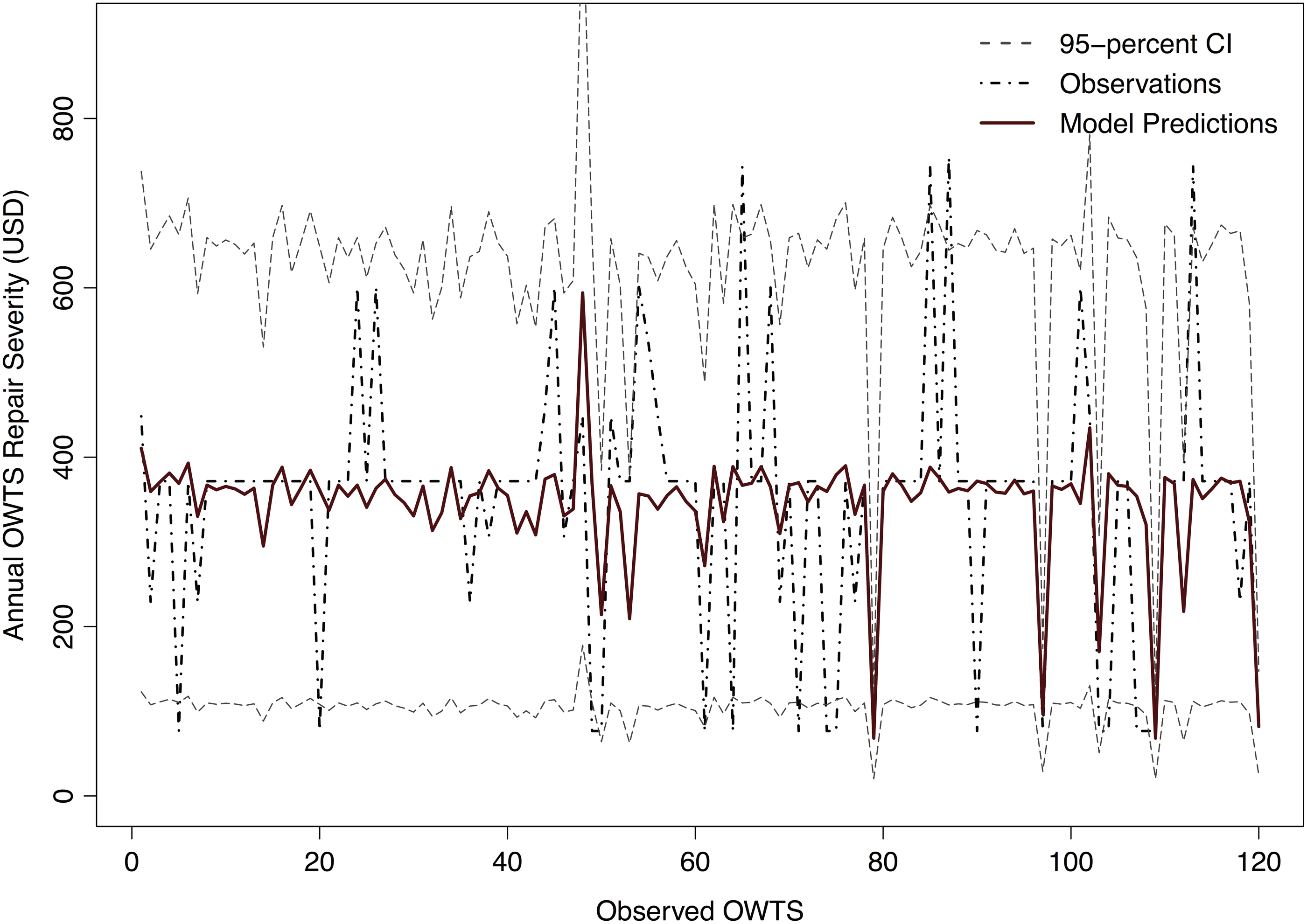
Predicted annual repair severity (USD) and 95% confidence limits using the fitted Weibull distribution parameters compared to the observed values for all 120 OWTS in the sample.

FIG. 4.

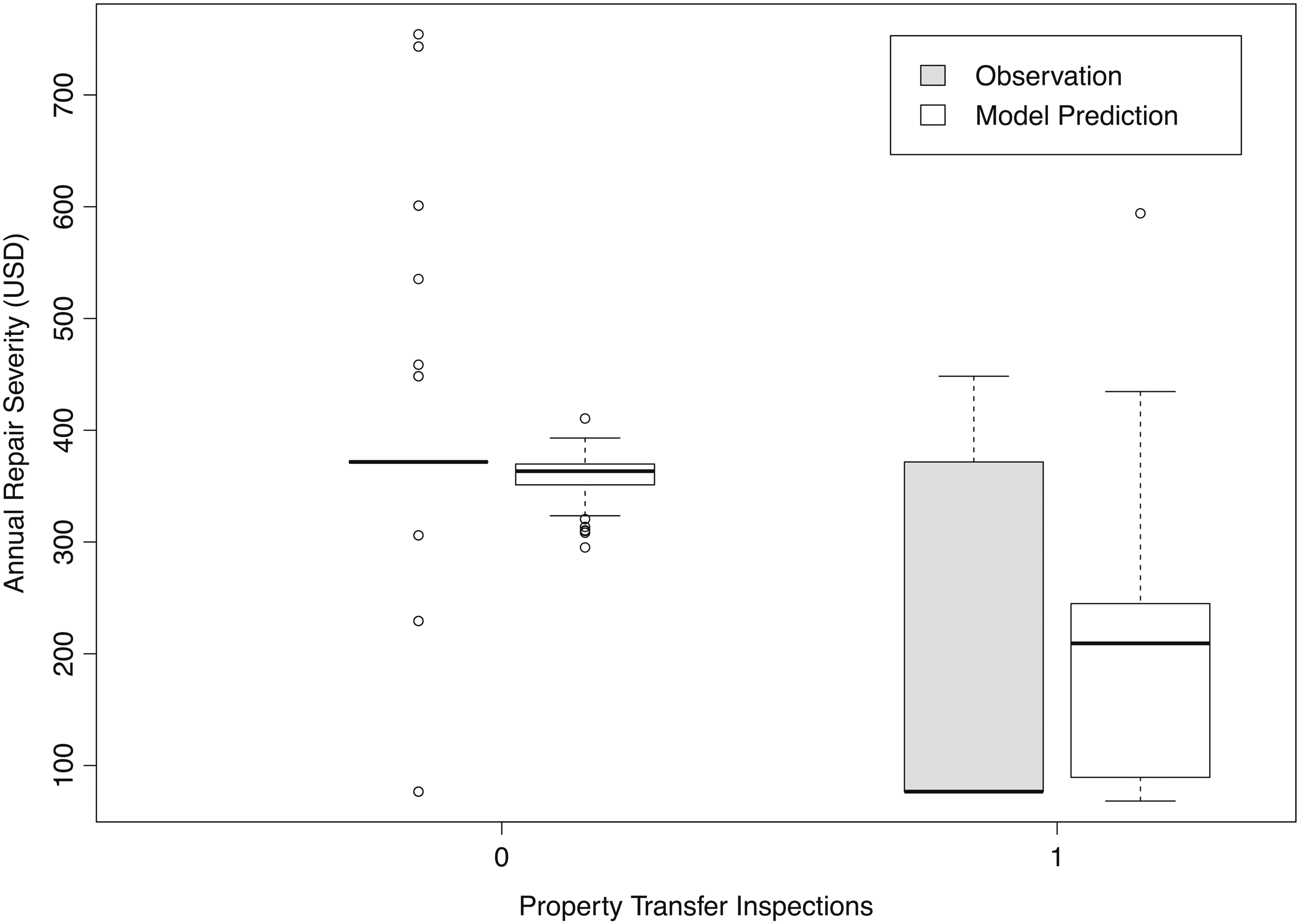
Relationship between predicted (Weibull) and actual annual repair severity costs and the number of property transfer inspections for 120 OWTS.

Figure 5 has spatial plots of the observed and predicted values of annual repair severity. While OWTS requiring moderate to major repairs are distributed throughout the County, the model does capture some spatial clustering of systems that had a history of higher cost repairs.

FIG. 5.

GIS map of observed annual repair severity (a) compared to the model estimates of annual repair severity (b). The windows zoom in on a selection of OWTS in and around the city of Boulder (refer to Fig. 1) to highlight the model's ability to capture annual repair severity based on the selected covariates.

As mentioned in the model description, the model residuals have to satisfy the assumption of normality, independence, and constant variance (i.e., homoscedasticity). These provide a set of measures for testing the model adequacy shown in Fig. 6. The histogram supports the assumption of normally distributed residuals, and the ACF is minimal suggesting independence of the residuals. The heteroscedasticity plot shows no clear trend in residuals as a function of the estimated value of Y. Some of the structure in this latter plot is perhaps due to the categorical nature of the data. From the autocorrelation plot, it is apparent that while the correlation appears to be minimal, there is significant autocorrelation at the first lag, that is, one residual is correlated with the other, indicative of spatial correlation. This could be due to local factors such as topography and age of the neighborhood. Hierarchical models, where the residuals are modeled as a spatial Gaussian process, are attractive alternatives to capturing the residual structure.

FIG. 6.

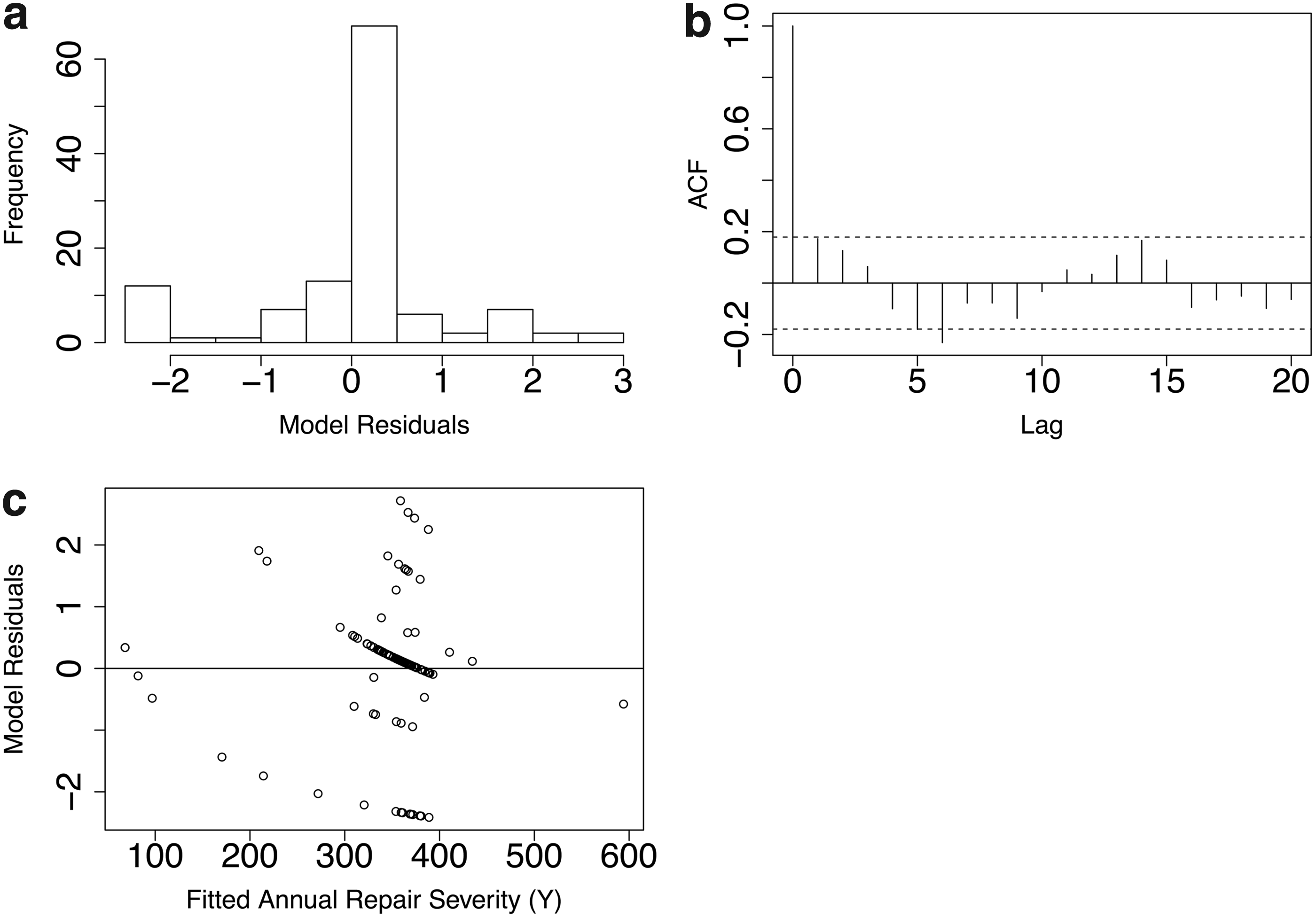
GAMLSS diagnostic plots. (a) Residuals histogram showing Normality, (b) Autocorrelation Function (ACF) distribution, and (c) constant variance plot of residuals testing for error heteroscedasticity.

Model cross-validation

The variability of the predicted RMSE and R² skill measures during cross-validation is shown as boxplots in Fig. 7. The relatively large variability in R² and RMSE is to be expected since the extremes cannot be modeled well without including them in the model fitting. The spread of both the skill indicators illustrates that the model is best applied to prediction within the original sample range and is least efficient in predicting extreme values of annual repair/replacement severity. The R² values of the cross-validation models range from approximately 0.1 to 0.8 and reflect the possibility that in each simulation some number of extreme values could be dropped resulting in under- or overprediction of annual repair severity. However, the low median RMSE value of ∼$134 indicates that a significant portion of the predictions differs only slightly from the annual repair severity observations, even after dropping 15% of the data.

FIG. 7.

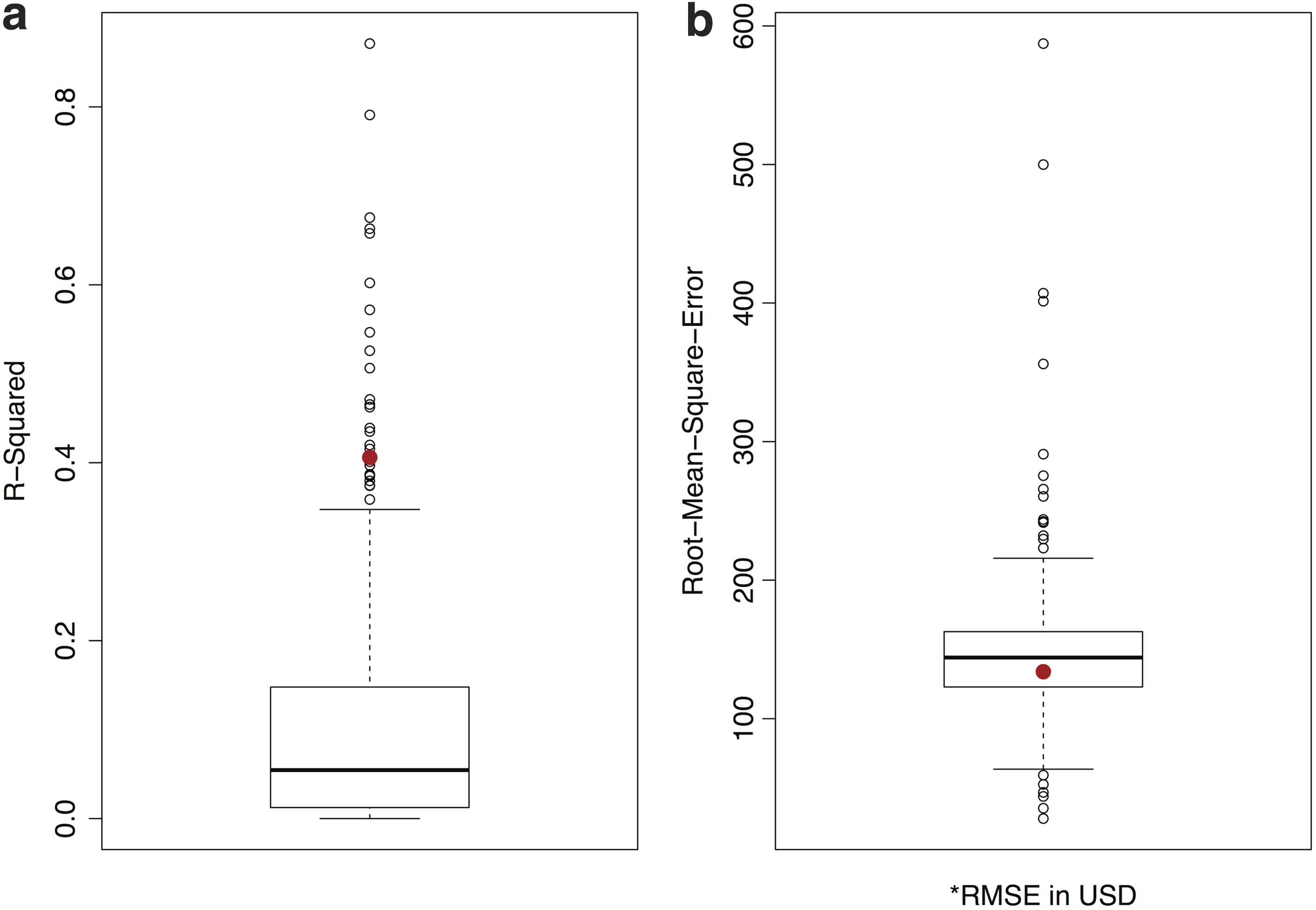
Skill of the Wiebull model of annual repair severity model skill as distributions of R² (a) and root mean squared error (RMSE) (b) of iterated regressions with 15% of observations dropped RMSE in hundreds of dollars. The red (plot in color) points are the R² and RMSE from the original reliability model.

Model sensitivity to cost estimates

Table 2 has the results of the sensitivity analysis comparing the original simulation (Model I), based on the average cost in each repair category to results from simulations using cost estimates in Models II and III. The covariates consistently associated with annual repair severity are UP, PT, PS, and the interaction between the number of upgrades and property transfer inspections (UP:PT). In addition, their influence on the likelihood of a high-cost annual repair severity is consistently negative with one exception in Model II where the likelihood of a high annual repair severity increases with an increased number of system upgrades. As the severity weighting is shifted using higher repair cost estimates, some of the covariates relevant in the initial GAMLSS, for example, LA, become insignificant to determining annual repair severity. However, the coefficient estimates of those variables in the initial model (Model I) are approximately zero, indicating that even in the initial model they have a lesser influence on annual repair severity than the highlighted more robust variables. Figure 8 shows the adjusted annual repair severity distributions based on the different cost estimates as well as the representative Weibull fit to each distribution. Figure 9 illustrates the sensitivity of the residuals of the GAMLSS to changes in cost estimates. Positive residuals in Fig. 9 indicate an overestimation of annual repair severity, whereas negative residuals reveal an underestimation of repair/replacement costs. Residuals based around zero demonstrate where the predicted value is close to the real annual repair severity value. In general, both positive and negative residuals increased along with cost estimates for both major and all repairs implying greater uncertainty in predictions of repair severity. This is not unexpected, as the predicted annual repair severity values also increase as a function of higher costs.

FIG. 8.

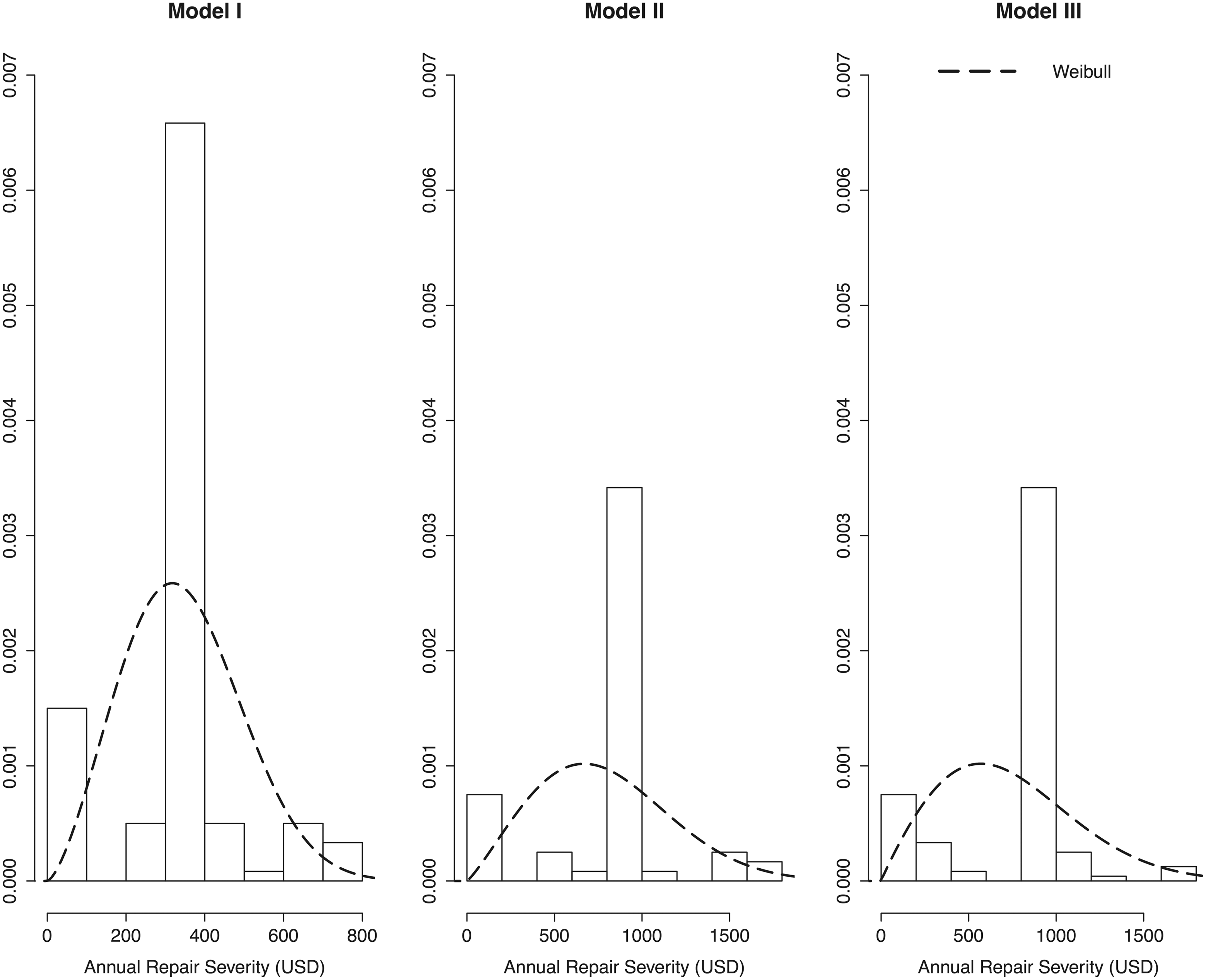
Estimated cost distributions for Models I, II, and III and their Weibull representation.

FIG. 9.

Sensitivity of model skill to repair cost estimates used to calculate annual repair severity. Model I is the original Weibull regression using the average of BCPH cost ranges for all repair categories; Model II is the Weibull regression substituting a higher cost estimate for major repairs; Model III is the Weibull regression with the higher cost estimate for all three categories of repairs.

Discussion

Public Good theory provides a policy framework for recommending increased regulation of OWTS (Mohamed, 2009). Health and environmental impacts of appreciable levels of OWTS failure and repair, aggravated by the growing density of these systems, are an additional motivation for new regulations requiring regular inspection and maintenance. However, new regulations have associated costs for both individual owners and for local health departments charged with maintaining records and processing permits. Results of this study provide data-based support for mandatory inspections that reduce repair frequency and cost over the OWTS life and a credible estimate of the benefits of increased oversight. In fact, the predicted benefit of inspections is conservative, since the Boulder County inspection/repair requirement only takes effect when a property is transferred. It may well be the case that a universal requirement for regular OWTS inspections through means such as a renewable permit would have an even larger benefit in improving OWTS reliability.

Two factors, SV and LA, have been considered as indicators of household affluence (Harlan et al., 2009). The GAMLSS showed a slight positive association of both with annual repair severity. Interestingly, this result goes against the common assumption that an increased ability to pay increases the likelihood of homeowner attention to maintenance and system performance. This counterintuitive result could be attributed to the location of these homes. In Boulder County, many larger high-value homes outside POTW service areas are located in mountainous areas far from maintenance services. Some may have STUs located in terrain, where a failure may not be noticed by either residents or neighbors. In addition, more expensive homes may be sold less often so that structural value is negatively related to mandatory inspections.

Finally, UP was associated with a decrease in predicted annual repair severity for OWTS. One explanation is that when a home's size is increased through remodeling and construction, the County requirement for expanded or appropriately upgraded systems would have an effect similar to property transfer inspections resulting in less frequent and less severe repairs. The relationship suggests that increasing system capacity also may benefit performance.

While individual variables such as inspections and repairs associated with property transfers, sales after 2008 and system upgrades decrease the likelihood of a high annual repair severity, inclusion of combined variables, especially those containing after 2008 property transfers, and improved the Weibull model skill. An interaction between individual variables with the same influence on the likelihood of a high annual repair severity amplifies those individual performance effects and increases the overall skill of the model. However, the small coefficient values for some of the combined variables such as structural value and regulated property transfers indicate that their effect on the expected value of annual repair severity was small. In general, LA and SV in combination with PT allow the model to discriminate between what might be considered a moderate range and a high range of annual repair severity values. While removing the two variables is an option given their p-values, they not only improve the skill of the model but also minimize GAIC compared to model versions without them. This indicates that while household affluence may not directly relate to annual repair severity, both indicator variables provide a nonarbitrary amplification of the highly significant covariate, PT, and capture the nonlinear effect of the interaction on OWTS performance.

Some spatial clustering of OWTS repair severity (Fig. 5) and autocorrelation of residuals (Fig. 6) suggest that not all factors determining OWTS failure are captured in the Weibull regression. Both geographic clustering and autocorrelation may be explained by factors such as weather, soil and groundwater conditions, and distance from OWTS servicers and from other residences. As an attractive extension of this research, the relationship between OWTS repair severity and location can be explored using spatial modeling of the GAMLSS residuals in a hierarchical modeling approach or a Bayesian method (e.g., Verdin et al., 2015). Another potential extension of this study exists in the discretized characteristic of the data (Fig. 2), which lends itself to a categorical modeling approach using a binomial or multinomial logistic regression analyses (e.g., Towler et al., 2013) to estimate risk, particularly quantifying the likelihood of high repair severity occurrences.

Summary

As the use of owner-operated on-site sanitation technologies increases, life cycle costs and long-term sustainability, including environmental and health impacts, become more relevant to reducing the risk of human and environmental exposure to wastewater contaminants. This research identified factors unique to minimally regulated OWTS that may guide future planning to enable better OWTS management over the system life. In the absence of comprehensive monitoring data, the product of the cost and frequency of system repairs and replacement, annualized over a 40-year lifetime, denoted as “annual repair severity,” is proposed as a measure of system failure. Data from 120 OWTS in Boulder County, Colorado, are fit by regression (GAMLSS) modeling, with the best fit provided by the Weibull distribution. In general, variables associated with more frequent owner management of OWTS were predictive of long-term system integrity. The most important was the frequency of inspections by professional servicers, typically accompanied by maintenance and minor repairs. This result suggests that mandatory inspections through a mechanism such as renewable permits would significantly reduce life cycle repair/failure frequency and severity, lowering OWTS costs to owners and reducing public exposure to wastewater contaminants. The statistical model is skilled at predicting repair severity in the midrange of the data distribution, with an expected annual repair/replacement cost between $350 and $400 per year, over the 40-year life cycle. The observed and modeled annual repair severity values were correlated with an R² value of 0.406, with larger discrepancies at the high values of annual repair severity, which fell in the range of $600 to $800 per year. The model dependence on inspection frequency as a principal determinant of repair severity was not sensitive to the cost estimates assigned to each category, indicating general applicability of the model results.

Footnotes

Acknowledgments

This material is based on work supported by the National Science Foundation Graduate Research Fellowship under Grant No. DGE 1144083. The authors would like to acknowledge the assistance of the staff of Boulder County Public Health Department who provided data and other information on OWTS in the Boulder County.

Author Disclosure Statement

No competing financial interests exist.

References

Akantziliotou

, Rigby

R.A.

, and Stasinopoulos

D.M.

(2002). The R implementation of generalized additive models for location scale and shape. In: Stasinopoulos

and Touloumi

(Eds.) Statistical Modelling in Society: Proceedings of the 17th International Workshop on Statistical Modelling. Chania, Greece.

Akaike

(1974). A new look at the statistical model identification. IEEE Trans. Automatic Trans., 19, 716.

BCPH. (2013). Boulder Coutny Public Health (BCPH) OWTS Repair Permit Data. Boulder, CO: BCPH.

Brown and Root Services. (2001). On-site Sewage Risk Assessment System. Bankstown: NSW Department of Local Government.

Burian

, Nix

, Pitt

, and Durrans

(2000). Urban wastewater management in the United States: Past, present, and future. J. Urban Technol., 7, 33.

Carroll

, Goonetilleke

, Thomas

, Hargreaves

, Frost

, and Dawes

(2006). Integrated risk framework for onsire wastewater treatment systems. Environ. Manage., 38, 286.

Chen

, and Herr

(2002). Comparison of BASINS and WARMF models: Mica Creek Watershed. Sytech Engineering, Inc. Electric Power Research Institute (EPRI), Palo Alto, CA and NCSAI Research Triangle Park, NC.

Cosgrove

(1909). History of Sanitation. Pittsburgh: Standard Sanitary Mfg. Co.

Crites

, and Tchobanoglous

(1998). Small and Decentralized Wastewater Management Systems. WCB McGraw-Hill Companies, Inc., Boston, MA.

10.

Cromer

(1999a). TRENCH 3.0 Preview: A computer application for site assessment and system sizing in Patterson, R. A. On-site '99 Conference: Making on-site wastewater systems work. Armidale: University of New England, pp. 85–88.

11.

Cromer

(1999b). TRENCH 3.0: An AIEH computer software application for managing on-site wastewater disposal. Environ. Health Rev. pp. 23–25.

12.

D'Amato

, Bahe

, Bounds

, Comstock

, Konsler

, Liehr

, et al. (2008). Factors Affecting the Performance of Primary Treatment in Decentralized Wastewater Systems. Alexandria: WERF & IWA.

13.

Dowdy

, Wearden

, and Chilko

(2004). Statistics for Research (3rd ed.). Hoboken, NJ: John Wiley & Sons, Inc.

14.

EPA. (1980). Design Manual: Onsite Wastewater Treatment and Disposal Systems. Office of Water. Washington, DC: EPA 625/1–80-012.

15.

EPA. (1997). Response to Congress on Use of Decentralized Wastewater Treatment Systems. U.S. EPA. Washington, DC.

16.

EPA. (1998). National Water Quality Inventory: 1996 Report to Congress. Washington, DC. EPA 841-R-97–008.

17.

EPA. (2002a). The Clean Water and Drinking Water Infastructure Gap Analysis. Office of Water. Cincinnati: U.S. EPA.

18.

EPA. (2002b). Onsite Wastewater Treatement Manual. U.S. EPA. Washington, DC.

19.

EPA. (2003). Voluntary National Guidelines for Management of Onsite and Clustered (Decentralized) Wastewater Treatment Systems. U.S. EPA. Washington, DC.

20.

EPA. (2008a). Septic System Fact Sheet. U.S. EPA. Washington, DC.

21.

EPA. (2008b). Enforcement and Compliance History Online (ECHO). Available at: <www.epa-echo.gov/echo/compliance_report_water.html> (accessed January 9, 2009).

22.

Etnier

, Pinkham

, Crites

, Johnstone

, Clark

, and Macrellis

(2007). Overcoming Barriers To Evaluation And Use Of Decentralized Wastewater Technologies And Management. Alexandria: WERF & IWA.

23.

Etnier

, Willetts

, Mitchell

, Fane

, and Johnstone

(2005). Decentralized Wastewater System Reliability Analysis Handbook. Project No. WU-HT-03–57. Prepared for the National Decentralized Water Resources Capacity Development Project, Washington University, St. Louis, MO, by Stone Environmental, Inc., Montpelier, VT.

24.

Furrer

, and Katz

(2007). “Generalized linear modeling approach to stochastic weather generators.” Climate Res. 34, 129.

25.

Hardin

(1968). The tragedy of the commons. Science. 162, 1243.

26.

Harlan

S.L.

, Yabiku

S.T.

, Larsen

, and Brazel

A.J.

(2009). Household water consumption in an arid city: affluence, affordance, and attitudes. Soc. Nat. Resour., 22, 691.

27.

Hudson

J.F.

(1986). Forecasting Onsire Soil Absorption System Failure Rates. Urban Systems Research & Engineering, Inc. Cincinnati: U.S. EPA.

28.

Hunter

J.E.

, and Schmidt

F.L.

(2004). Methods of Meta-Analysis: Correcting Error and Bias in Research Findings. Sage Publications, Inc. Thousand Oaks, CA.

29.

Joubert

, Hickey

, Kellogg

, and Gold

(2004). Wastewater Planning Handbook: Mapping Onsite Treatment Needs, Pollution Risks, and Management Options Using GIS. Univerity of Rhode Island, Cooperative Extension. Kingston: National Decentralized Water Resources Capacity Development Project (NDWRCDP).

30.

Kaminsky

, and Javernick-Will

(2013). Contested factors of sustainability: Construction and management of household on-site wastewater treatment systems. J. Constr. Eng. Manage., 139, A4013004.

31.

Katz

R.W.

, Bush

G.S.

, and Naveau

(2002). Statistics of extremes in hydrology. Adv. Water Resour., 25, 1287.

32.

Kenway

, and Irvine

(2001). Sewage Pollution Risk Assessment for Environmental Health. Environmental Health Conference. Bathurst.

33.

Kleiber

, Katz

, and Rajagopalan

(2012). “Daily spatiotemporal precipitation simulation using latent and transformed Gaussian processes.” Water Resour. Res., 48, 1.

34.

Kleiber

, Katz

, and Rajagopalan

(2013). “Daily minimum and maximum temperature simulation over complex terrain.” Ann. Appl. Stat., 7, 588.

35.

“LA Sewers.”. LA Sewers. City of Los Angeles Department of Public Works. (2013). Available at: <http://lasewers.org/private_sewers_septic/septic_systems/index.htm> (accessed April 29, 2015.)

36.

Mayer

, and DeOreo

(1999). Residential End Uses of Water. American Water Works Association (AWWA), American Water Works Association Research Foundation (AWWARF). AWWA. Denver, CO.

37.

McCullagh

, and Nelder

(1989). Generalized Linear Models (2nd Edition ed.). Chapman: Hall/CRC, London.

38.

McKinley

J.W.

, and Siegrist

R.L.

(2011). Soil clogging genesis in soil treatment units used for onsite wastewater reclamation: a review. Crit. Rev. Environ. Sci. Technol., 41, 2186.

39.

McGuinness

, and Martens

(2003). GIS-based model to assess potenital risk of individual onsite effluent management systems: development Assessment Module (DAM). Onsite '03 Conference: Future directiosn for onsite systems-Best management practices. Armidale: University of New England, pp. 265–271.

40.

Mohamed

(2009). Why households in the United States do not maintain their septic systems and why state-led regulations are necessary: explanations from public goods theory. Int. J. Sustainable Dev. Plann., 4, 42.

41.

Nauges

, and Van den Berg

(2006). Water Markets, Demand and Cost Recovery for Piped Water Supply Services: Evidence from Southwest Sri Lanka. Water and Sanitation Programme (WSP) of the World Bank. Washington, DC.

42.

Nieswiadomy

, and Molina

(1989). Comparing residential water demand estimates under decreasing and increasing block rates using household data. Land Econ. 65, 280.

43.

Oosting

, and Joy

(2011). A GIS-based model to assess the risk of on-site wastewater systems impacting groundwater and surface water. Can. Water Resour. J., 36, 229.

44.

Rigby

, and Stasinopoulos

(2005). Generalized additive models for location, scale and shape. Appl. Stat., 54, 507.

45.

Rigby

, and Stasinopoulos

(2001). The GAMLSS project: a flexible approach to statistical modelling. 16th International Workshop on Statistical Modeling. Odense, pp. 249–256.

46.

“SepticSmart Program.”. SepticSmart Program. Boulder County Colorado. (2015). Available at: <www.bouldercounty.org/env/water/pages/septicsmartindex.aspx> (accessed April 29, 2015).

47.

Stasinopoulous

, Ridby

, and Akantziliotou

(2008). Instructions on how to use the gamlss package in R. www.gamlss.org/wp-content/uploads/2013/01/gamlss-manual.pdf

48.

Towler

, Roberts

, Rajagopalan

, and Sojda

(2013). Incorporating probabilistic seasonal climate forecasts into river management using a risk-based framework. Water Resour. Res., 49, 4997.

49.

Turvey

(1963). On divergences between social cost and private cost. Economica. 30, 309.

50.

U.S. Census Bureau. (2006). American Housing Survey for the United States: 2005.Washington DC, 2006.

51.

U.S. Census Bureau. State and County Quick Facts. (2015). Available at: http://quickfacts.census.gov/qfd/states/08/08013.html (accessed September 27, 2015.)

52.

Verdin

, Rajagopalan

, Kleiber

, and Funk

(2015). A Bayesian kriging approach for blending satellite and ground precipitation observations. Water Resour. Res., 51, 908.

53.

Weirich

, Silverstein

, and Rajagopalan

(2011). Effect of average flow and capacity utilization on effluent water quality from US municipal wastewater treatment facilities. Water Res. 45, 4279.

54.

Weirich

, Silverstein

, and Rajagopalan

(2015). Resilience of secondary wastewater treatment plants: prior performance is predictive of future process failure and recovery time. Environ. Eng. Sci., 32, 222.