Modeling Total Organic Carbon Variation in a Photocatalytic Process via Stochastic Differential Equations

Abstract

Advanced oxidative processes (AOP) are an important alternative in the treatment of industrial effluents. Several studies in the literature report that the kinetic profile of organic matter oxidation presents behavior typical of pseudo-first-order reactions. Recent work indicates a conversion rate in two phases: (1) a rapid initial phase described in pseudo-first-order kinetics and (2) a decelerated phase described as pseudo-first order. Previously published work proposed an empirical stochastic model that reproduced these behaviors. In the present study, we found the average conversion degradation calculated by the stochastic model can approximate this dual-reaction rate behavior. This model thus presents a method for estimating the apparent kinetics constant from the model parameters without the need to arbitrarily separate the two conversion stages in the same oxidation process. Additionally, the model's capability to describe the conversion of organic load for different types of effluents and processes showed that this model satisfactorily describes total organic carbon conversion for three different waste (leachate, dairy, and a synthetic one involving benzoic acid) handled by different AOP. Thus, this work evidenced that the proposed model can describe diversified oxidation processes combined with the carbonaceous charge degradation contained in complex industrial effluents.

Introduction

Recent studies have applied advanced oxidative processes (AOPs) to partial or total reduction of organic load of dairy effluents (Almeida et al., 2004; Pan et al., 2006; Villa et al., 2007; Banu et al., 2008). Villa et al. (2007) evaluated Photo-Fenton/solar process efficiency in the reduction of organic load from dairy effluents of a dairy industry in the city of São Carlos, State of São Paulo, Brazil, with the aim of applying a pretreatment phase or emergency treatment. When the process efficiency was analyzed for different organic loads, total organic carbon (TOC) of 350, 2,500 and 5,000 mg/L, a TOC reduction of 90, 86, and 50, respectively, was observed, for a radiation time of 3.5 h.

Due to the complexity of recalcitrant industrial wastewater, where there is concomitant formation and degradation of various organic groups by oxidative processes, it is difficult to estimate a definite kinetic order. This problem has been discussed by other authors, for example, Orbeci et al. (2014) and Chen et al. (2011). Those authors reported antibiotics and benzoic acid degradation by photo-Fenton in two distinct phases: the first one, occurring within 10 min with a greater reaction rate (Kc₁ in the range of 10⁻¹ s⁻¹) and the second one, with a lower rate (Kc₂ in the range of 10⁻² s⁻¹). Two distinct phases were also observed by Siqueira et al. (2013) working with dye and textile effluents.

The stochastic model, here proposed, may distinguish different oxidation process phases (distinct conversion rates, including apparent reaction rate estimation). The first phase, normally with a very fast reaction, followed by a second phase, with a slower reaction rate. This double behavior is crucial, since changes in the reaction conditions of the oxidative process may influence it. Reaction conditions may include, for example, changes in reagent input flow rates, so there is no consumption of radical oxidants and/or low oxidation of the carbonaceous charge (Loures et al. 2013).

Although design of experiments (DOE) is a traditional technique for degradation of effluents by AOP modeling, it usually uses only the last data information (percentage of total degradation) obtained in each experiment of the matrix planning. Thus, a large amount of information is not used in process optimization via DOE modeling (e.g., response surface). Another important fact is that the response variables, such as chemical oxygen demand (COD), are susceptible to physical and chemical interferences. Such interference may mask the experimental measurements. A proposal to minimize these problems is presented in Siqueira et al. (2013), based on stochastic modeling. In this approach, the authors proposed an empirical model to predict the effluent degradation kinetic profile as a function of time as well as a confidence interval (CI) for the measurements for various types of industrial wastewater treated by AOP. This innovative approach has already been successfully tested on dye and textile effluents, considering COD as response variable (Siqueira et al., 2013).

This study aims to evaluate the stochastic model adjustment on describing TOC conversion for AOP-treated effluents. A comparison of model parameters relating to organic load oxidation kinetic constants is presented. In this sense, we presented a methodology for estimating these constants considering two distinct phases: a fast initial followed by a slower one. As an example, the adjustment of model is evaluated for two real effluents (dairy industry and leachate), as well as for literature experimental data (benzoic acid).

To evaluate the model, three effluents treated with different AOPs were analyzed. The choice of these effluents was due to the availability of experimental data for analysis. First, data from leachate degradation by AOP (catalytic ozonation) were analyzed. During the effluent treatment, a good density of experimental data was obtained at the beginning of the reaction.

Catalytic ozonation has shown to be effective in the removal of several organic compounds present in water and aqueous effluents. The reaction mechanism is the transfer of electrons from the metal reduced to ozone, forming Fe³⁺ ion and radical ion O₃⁻, and hydroxyl radical. In the presence of excess Fe²⁺, hydroxyl radical can oxidize a second Fe²⁺, providing a stoichiometric ratio of 0.5 moles of ozone per mole of ferrous ion (Loures et al., 2013).

Second, data, as shown in Fig. 2 of Chen et al. (2011), were extracted (digitalized) and analyzed. In this work, a synthetic effluent (benzoic acid) was treated by AOP (Fenton). Authors for such work give estimates of kinetic constants, k_obs1 and k_obs2 (here denominated as kc₁ and kc₂, respectively). These constants were compared to those estimated by the proposed technique of this article.

Efficiency of global reaction in the Fenton process is credited to the relationship among [Fe⁺²], [Fe⁺³], [H₂O₂], and characteristics of reaction medium (pH, temperature and amount of organic and inorganic constituents). In Fenton reaction, hydroxyl radicals are generated from the reduction of hydrogen peroxide, with a significant reaction rate (k = 76 L/[mol·s]). In this case, iron acts as a catalyst and is oxidized. Concomitantly, reduction of Fe³⁺ with H₂O₂ occurs, which is usually much slower than the oxidation of Fe²⁺. So, the iron exists in solution mostly in the form of Fe³⁺. Hydrogen peroxide can also act as a consumer of hydroxyl radicals, forming hydroperoxide radicals (HO₂^•). These species have a lower standard reduction potential (E° = 1.42 V) in comparison to ^•OH and the formation occurs mainly in the presence of excess H₂O₂. In this case, Fe²⁺ concentration in the reaction medium is low in relation to that of Fe³⁺, producing a slower reaction. This occurs due to the reaction between Fe³⁺ and H₂O₂ and it is slower than the decomposition of H₂O₂ in the presence of Fe²⁺ (Loures et al., 2013).

Finally, dairy effluent modeling treated by photo-Fenton was presented. On this effluent, 180 tests measuring concentration of TOC were carried out. The high number of determinations permitted to compare the distribution of probability of the stochastic model was proposed with the distribution of empirical probability generated by experimental data through the pseudo-residual technique (Zucchini and MacDonald, 2009).

In photo-Fenton reaction, Fe²⁺/Fe³⁺ is used in the presence of hydrogen peroxide under irradiation. Photon absorption by ferric ions can extend into the visible region of spectrum, depending on pH and ligands. pH influences the formation of hydroxylate species, which has a higher absorption in the visible spectrum. Among various iron complexes, the species Fe(OH)²⁺ shows maximum absorbance at about 300 nm extending to 400 nm, which enables solar-irradiated photo-Fenton reactions. Many photochemical reactions may occur in the photo-Fenton system, depending on the emission spectrum of the radiation source and on the absorbance of existing chemical species. The photolysis of H₂O₂, which generates two hydroxyl radicals, can occur simultaneously with the photo-Fenton reaction. However, its low molar absorption coefficient (18.7 L/[mol·cm] at 254 nm) makes this phase less important in the photo-Fenton process, especially, if one considers the absorption of light by iron and organic compounds (Loures et al., 2013).

Some characteristics have been emphasized to understand the challenges presented in a single model that is used to understand the effluent degradation process with several AOPs.

Chemical and microbiological composition of leachate formed in a sanitary landfill is complex and depends on several factors, such as environmental conditions, residue composition over the landfill, landfill management, and mainly, the dynamics of the decomposition process that occurs within cells in a sanitary landfill (Kjeldsen et al., 2002).

Variable composition of landfill residues can produce a percolate with high toxic metal content, xenobiotics (unknown substances to live organisms), and microorganisms that represent a risk to health (Baun et al., 2004). Leachates are composed of organic and inorganic matter. Organic fractions contain proteins, amides, amines, fat, organic acids, sugars, and other products of residue decomposition. Chemical substances contained in several product wrappers, especially cleaning products and pesticides, contribute significantly to the formation of leachate. Vegetal decomposition or wooden residues on landfills also contribute to the presence of humid compounds that are hardly degradable. The dairy segment in Brazil is relevant in the agro industrial sector, not only for commercial but also due to high pollutants (IEA, 2011; Salazar and Izário Filho, 2009). Liquid effluents of this type of industry comprised washing water from equipment and floors, sanitary sewage generated, and milk and derivative products. The generation of liquid effluents from this sector is related to the volume of water consumed, in which every liter of milk generated about 2.5 L of effluent (Pupo Nogueira et al., 2007). Effluent generated by dairy products in the milk process contains a COD of about 3,000 mg/L. In sectors with high production of cheese and derivative, the COD value is higher than 50,000 mg/L (Gavala et al., 1999). From this amount, the lipid content is higher than 100 mg/L (Hwu et al., 1998).

Dairy effluents have great amount of lipids, carbohydrates, and proteins giving the system a high organic load. They have high COD and biochemical oxygen demand (BOD₅). It is common to find values up to 10,000 and 2.50 mg/L for COD and BOD₅, respectively. In addition, a DBO₅/COD ratio of about 0.25 may be found. According to Malato et al. (2000), this ratio should be higher than 0.4 to be considered a biodegradable effluent. When disposed in water bodies, without appropriate treatment, it may reduce dissolved oxygen concentration with serious risks to the aquatic ecosystems (Cordi et al., 2008).

Several chemical, physical, and biological process techniques to treat effluents are available, as well as the combination of all these processes. However, each process has its own limitation in terms of implementation, efficiency, and costs. For this reason, it is necessary to develop the use of efficient and cheap technologies (Rey et al., 2009).

Mathematical Model

The empirical stochastic differential equation (SDE) proposes to study the variation of TOC, which is given by Equation (1) in this work, and was first studied by Siqueira et al. (2013).

In this equation, the first part represents the chemical conversion tendency for a long time. The second part represents Brownian movement modeling data dispersion (W_t). \documentclass{aastex}\usepackage{amsbsy}\usepackage{amsfonts}\usepackage{amssymb}\usepackage{bm}\usepackage{mathrsfs}\usepackage{pifont}\usepackage{stmaryrd}\usepackage{textcomp}\usepackage{portland, xspace}\usepackage{amsmath, amsxtra}\pagestyle{empty}\DeclareMathSizes{10}{9}{7}{6}\begin{document} \begin{align*} {{\rm dX}_{t}} = \left( {\rm a} + {\frac {b \cdot k} {e^ {k \cdot t}}} \right) {\rm dt} + {\frac {c} {{\rm (t + 1)}^p}} {\rm dW}_{t } \tag {1} \end{align*} \end{document}

Where a, b, c, k, and p are parameters of the model and depend on experimental conditions. X_t is the conversion of TOC at time t, in minutes. The heuristic for this proposal can be found in the properties of Equation (1). This equation shows the following properties: For each t > 0, X_t has a normal distribution with mean and variance given by [Eqs. (2 and 3)]. \documentclass{aastex}\usepackage{amsbsy}\usepackage{amsfonts}\usepackage{amssymb}\usepackage{bm}\usepackage{mathrsfs}\usepackage{pifont}\usepackage{stmaryrd}\usepackage{textcomp}\usepackage{portland, xspace}\usepackage{amsmath, amsxtra}\pagestyle{empty}\DeclareMathSizes{10}{9}{7}{6}\begin{document} \begin{align*} E (X_{t}) = a \times t + b ({1} - {e}^{- k \times t}) = { \mu _t} \tag{2}\end{align*} \end{document} \documentclass{aastex}\usepackage{amsbsy}\usepackage{amsfonts}\usepackage{amssymb}\usepackage{bm}\usepackage{mathrsfs}\usepackage{pifont}\usepackage{stmaryrd}\usepackage{textcomp}\usepackage{portland, xspace}\usepackage{amsmath, amsxtra}\pagestyle{empty}\DeclareMathSizes{10}{9}{7}{6}\begin{document} \begin{align*} { \rm Var } \left( { { X_t } } \right) = { \frac { { c^2 } } { 2p - 1 } } \cdot \left( { 1 - \frac { 1 } { { { { \left( { { \rm t } + 1 } \right) } ^ { 2p - 1 } } } } } \right) = \sigma _t^2 \tag { 3 } \end{align*} \end{document}

To make the model clearer, a scheme of parameter meaning is shown in Fig. 1.

FIG. 1.

Schematic representation of the model.

Figure 1 was plotted to better understand how model parameters influence the reaction. Parameter a defines the slope of the plateau that the reaction attains after the initial rapid conversion reaction. Parameter b marks the baseline mean value of conversion at which the effect begins. Parameters c and p relate to the dispersions and correlation of experimental data. Parameter k is related to the reaction time required to reach a plateau. By Equation (2), it can be observed for k large that the average shape of the curve shows a fast exponential growth, stabilizing at a plateau with initial value of the b parameter. After reaching this plateau, the expected value presents a linear behavior, modeled by the term a × t. In all the experimental runs analyzed, the value of the parameter is very small and in many cases, zero, considering the CI of the parameter.

Based on the model, it makes possible to approach the reaction time to reach the plateau (tpat), for k large, with the following simple Equation (4). \documentclass{aastex}\usepackage{amsbsy}\usepackage{amsfonts}\usepackage{amssymb}\usepackage{bm}\usepackage{mathrsfs}\usepackage{pifont}\usepackage{stmaryrd}\usepackage{textcomp}\usepackage{portland, xspace}\usepackage{amsmath, amsxtra}\pagestyle{empty}\DeclareMathSizes{10}{9}{7}{6}\begin{document} \begin{align*} { \rm tpat } = \frac { { 2. \ln \left( { 10 } \right) } } { k } \tag { 4 } \end{align*} \end{document}

Alternatively, tpat may be better estimated by the root of Equation (5). \documentclass{aastex}\usepackage{amsbsy}\usepackage{amsfonts}\usepackage{amssymb}\usepackage{bm}\usepackage{mathrsfs}\usepackage{pifont}\usepackage{stmaryrd}\usepackage{textcomp}\usepackage{portland, xspace}\usepackage{amsmath, amsxtra}\pagestyle{empty}\DeclareMathSizes{10}{9}{7}{6}\begin{document} \begin{align*} a \times t - b \times {e^{ - k \times t}} = 0 \tag{5} \end{align*} \end{document}

On Equation (3), it can be observed that the variability in the initial time of X_t is zero. This agrees with the initial conversion to be zero. Moreover, the variance grows of X_t that depends on the constants c and p. This behavior was also evident in the experimental runs analyzed from different types of effluent treated with AOPs. The growth rate of variability depends on the constant p. Finally, the presence of Brownian movement is justified in the existence of the phenomenon of interference between the reactants of POA that can lead to reading errors of TOC (or COD) at a given time, as discussed in the Introduction section.

The methodology to find parameters a, b, k, and p is described in the function of experimental data in Siqueira et al. (2013). The main idea comes from an initial guess for k parameter, typically k ∈ (0,2); the algorithm developed by Siqueira et al. (2013) may estimate the parameters of the model as well as the error margin. The algorithm is based on techniques for estimating SDE (Kelly et al., 2004) and sampling, called Bootstrap (Efron and Tibshirani, 1993). Parameter c, however, presented a slight modification on the estimator shown by Siqueira et al. (2013). The difference is based on the response variable TOC, in which the estimator of c is divided by 15 (Equation 6). \documentclass{aastex}\usepackage{amsbsy}\usepackage{amsfonts}\usepackage{amssymb}\usepackage{bm}\usepackage{mathrsfs}\usepackage{pifont}\usepackage{stmaryrd}\usepackage{textcomp}\usepackage{portland, xspace}\usepackage{amsmath, amsxtra}\pagestyle{empty}\DeclareMathSizes{10}{9}{7}{6}\begin{document} \begin{align*} { \rm c } = \frac { 1 } { { 15 } } \sqrt { { \frac { \sum { Q_i } } { \sum \frac { 1 } { { { { \left( { { t_i } + 1 } \right) } ^p } } } } } } \tag { 6 } \end{align*} \end{document}

Where Q_i (it may roughly be considered as a point measure of the data quadratic variation rate), being calculated as Equation (7). \documentclass{aastex}\usepackage{amsbsy}\usepackage{amsfonts}\usepackage{amssymb}\usepackage{bm}\usepackage{mathrsfs}\usepackage{pifont}\usepackage{stmaryrd}\usepackage{textcomp}\usepackage{portland, xspace}\usepackage{amsmath, amsxtra}\pagestyle{empty}\DeclareMathSizes{10}{9}{7}{6}\begin{document} \begin{align*} { Q_i } = { \frac { { { \left( { \Delta { { \rm X } _i } } \right) } ^2 } } { \Delta { { \rm t } _i } } } \tag { 7 } \end{align*} \end{document}

Numerical simulation of an SDE

In this work, the algorithm used to obtain numerical simulations of Equation (1) is according to the Euler–Maruyama method, which is easy to implement. Equation (1) can be discretized as Equation (8). \documentclass{aastex}\usepackage{amsbsy}\usepackage{amsfonts}\usepackage{amssymb}\usepackage{bm}\usepackage{mathrsfs}\usepackage{pifont}\usepackage{stmaryrd}\usepackage{textcomp}\usepackage{portland, xspace}\usepackage{amsmath, amsxtra}\pagestyle{empty}\DeclareMathSizes{10}{9}{7}{6}\begin{document} \begin{align*} { X_ { { \rm n } + 1 } } = { { \rm X } _n } + \left( { { \rm a } + { \frac { b \cdot k } { { e^ { k \cdot { { \rm t } _n } } } } } } \right) \Delta { { \rm t } _n } + \frac { c } { { { { \left( { { t_n } + 1 } \right) } ^p } } } \Delta { { \rm W } _n } \tag { 8 } \end{align*} \end{document}

In Equation (8), ΔW_n represents the increment of Wiener process, which can be calculated by a normal distribution with zero mean and variance Δt_n. Note that in Equation (8), all necessary information to estimate the value of X_n+1 depends only on the information at time t_n. In all simulations, the value of Δt_n was 0.01. All simulations were performed with SciLab5.5.2.

Confidence intervals

CIs are important tools to estimate parameters and to study the variability of the process X_t. Based on the Equation (3) for each time t, one can calculate a CI with 95% confidence for the process X_t by Equation (9). \documentclass{aastex}\usepackage{amsbsy}\usepackage{amsfonts}\usepackage{amssymb}\usepackage{bm}\usepackage{mathrsfs}\usepackage{pifont}\usepackage{stmaryrd}\usepackage{textcomp}\usepackage{portland, xspace}\usepackage{amsmath, amsxtra}\pagestyle{empty}\DeclareMathSizes{10}{9}{7}{6}\begin{document} \begin{align*} CI = E \left( {{X_t}} \right) \pm 1.96 \times dp \left( {{X_t}} \right) \tag{9} \end{align*} \end{document}

Where dp (X_t) is the square root of the Equation (3) and E(X_t) is the expected value for TOC conversion.

Thus, this work aims to extend the validation of the model proposed by Siqueira et al. (2013) for another type of effluent, besides developing new model properties and emphasizing its characteristics as a tool for AOP degradation analysis. Since the model utilizes the global information set, it makes possible to utilize the global information set to estimate individual analytic and operational measures, even though, some of them were influenced by physical or chemical interferences.

Therefore, the authors expect that the empirical stochastic model here proposed may be utilized for other types of distinct and complex industrial and natural effluents, without previous knowledge of its total composition.

Kinetical approach

This approach is presented to interpret the proposed model parameters relating to the kinetic constants (kc), as well as to propose a methodology to estimate these constants from the stochastic model (Kc). As mentioned in the Introduction section of this article, some authors reported that the treatment of different effluent types by AOP follows a pseudo-first-order behavior. Orbeci et al. (2014) and Chen et al. (2011) verified a high-order apparent reaction constant, kc₁ at the beginning of the treatment followed by another pseudo-first-order reaction, but with a low kinetic constant, kc₂. This double behavior can be approximated to the mean value of the first stochastic model at the beginning of the reaction and then to times close to tpat.

For a pseudo-first-order reaction, with kinetic constants (kc₁ and kc₂), the concentration variation rate may be approximated by Equation (10). \documentclass{aastex}\usepackage{amsbsy}\usepackage{amsfonts}\usepackage{amssymb}\usepackage{bm}\usepackage{mathrsfs}\usepackage{pifont}\usepackage{stmaryrd}\usepackage{textcomp}\usepackage{portland, xspace}\usepackage{amsmath, amsxtra}\pagestyle{empty}\DeclareMathSizes{10}{9}{7}{6}\begin{document} \begin{align*} { \frac { d { C_t } } { dt } } \approx - kc \times { C_t } \tag { 10 } \end{align*} \end{document}

Therefore, the conversion of C_t, for a small interval of time can be approximated to Equation (11). Thus, the mean conversion in a pseudo-first-order reaction is close to a linear behavior [Equation (11)]. \documentclass{aastex}\usepackage{amsbsy}\usepackage{amsfonts}\usepackage{amssymb}\usepackage{bm}\usepackage{mathrsfs}\usepackage{pifont}\usepackage{stmaryrd}\usepackage{textcomp}\usepackage{portland, xspace}\usepackage{amsmath, amsxtra}\pagestyle{empty}\DeclareMathSizes{10}{9}{7}{6}\begin{document} \begin{align*} {X_t} \approx \left( {1 - {e^{ - Kc \times t}}} \right) \approx Kc \times t \tag{11} \end{align*} \end{document} \documentclass{aastex}\usepackage{amsbsy}\usepackage{amsfonts}\usepackage{amssymb}\usepackage{bm}\usepackage{mathrsfs}\usepackage{pifont}\usepackage{stmaryrd}\usepackage{textcomp}\usepackage{portland, xspace}\usepackage{amsmath, amsxtra}\pagestyle{empty}\DeclareMathSizes{10}{9}{7}{6}\begin{document} \begin{align*} E \left( {{X_t}} \right) \approx Kc \times t \tag{12} \end{align*} \end{document}

The stochastic model [Equation (1)] also shows a linear-like behavior to mean conversion at the beginning of the treatment to t lower case as shown in Equation (13). \documentclass{aastex}\usepackage{amsbsy}\usepackage{amsfonts}\usepackage{amssymb}\usepackage{bm}\usepackage{mathrsfs}\usepackage{pifont}\usepackage{stmaryrd}\usepackage{textcomp}\usepackage{portland, xspace}\usepackage{amsmath, amsxtra}\pagestyle{empty}\DeclareMathSizes{10}{9}{7}{6}\begin{document} \begin{align*} E \left( {{X_t}} \right) = a \times t + b \left( {1 - {e^{ - k \times t}}} \right) \approx \left( {a + b \times k} \right) t \tag{13} \end{align*} \end{document}

Thus, an estimate to Kc₁ using the stochastic model parameters would be given in Equation (14). \documentclass{aastex}\usepackage{amsbsy}\usepackage{amsfonts}\usepackage{amssymb}\usepackage{bm}\usepackage{mathrsfs}\usepackage{pifont}\usepackage{stmaryrd}\usepackage{textcomp}\usepackage{portland, xspace}\usepackage{amsmath, amsxtra}\pagestyle{empty}\DeclareMathSizes{10}{9}{7}{6}\begin{document} \begin{align*} K{c_1} \approx \left( {a + b \times k} \right) \tag{14} \end{align*} \end{document}

However, as Equation (14) is only an estimate, another procedure was proposed to obtain a better adjustment to Kc₁. This procedure of effluent analyses seems to be the best in this work. In this study, the initial concentration (C₀) is considered as being constant. Conversion definition (C_t) is described as in Equation (15). \documentclass{aastex}\usepackage{amsbsy}\usepackage{amsfonts}\usepackage{amssymb}\usepackage{bm}\usepackage{mathrsfs}\usepackage{pifont}\usepackage{stmaryrd}\usepackage{textcomp}\usepackage{portland, xspace}\usepackage{amsmath, amsxtra}\pagestyle{empty}\DeclareMathSizes{10}{9}{7}{6}\begin{document} \begin{align*} {C_t} = {C_0} - {C_0}{X_t} \tag{15} \end{align*} \end{document}

This variable differential may be calculated by Equation (16). For Equation (16), it is possible to calculate the differential of the expected value for the concentration in instant t, E(C_t), resulting in Equation (17). \documentclass{aastex}\usepackage{amsbsy}\usepackage{amsfonts}\usepackage{amssymb}\usepackage{bm}\usepackage{mathrsfs}\usepackage{pifont}\usepackage{stmaryrd}\usepackage{textcomp}\usepackage{portland, xspace}\usepackage{amsmath, amsxtra}\pagestyle{empty}\DeclareMathSizes{10}{9}{7}{6}\begin{document} \begin{align*} d { C_t } = - { C_0 } \times d { X_t } = - { C_0 } \left( { \left( { a + { \frac { b \times k } { { e^ { k \times t } } } } } \right) dt + \frac { c } { { { { \left( { 1 + t } \right) } ^p } } } d { W_t } } \right) \tag { 16 } \end{align*} \end{document} \documentclass{aastex}\usepackage{amsbsy}\usepackage{amsfonts}\usepackage{amssymb}\usepackage{bm}\usepackage{mathrsfs}\usepackage{pifont}\usepackage{stmaryrd}\usepackage{textcomp}\usepackage{portland, xspace}\usepackage{amsmath, amsxtra}\pagestyle{empty}\DeclareMathSizes{10}{9}{7}{6}\begin{document} \begin{align*} dE \left( { { C_t } } \right) = - { C_0 } \left( { a + { \frac { b \times k } { { e^ { k \times t } } } } } \right) dt \tag { 17 } \end{align*} \end{document}

Calculating once more the expected value in Equation (15) and isolating C₀, the following Equation (18) is obtained. \documentclass{aastex}\usepackage{amsbsy}\usepackage{amsfonts}\usepackage{amssymb}\usepackage{bm}\usepackage{mathrsfs}\usepackage{pifont}\usepackage{stmaryrd}\usepackage{textcomp}\usepackage{portland, xspace}\usepackage{amsmath, amsxtra}\pagestyle{empty}\DeclareMathSizes{10}{9}{7}{6}\begin{document} \begin{align*} { C_0 } = { \frac { E \left( { { C_t } } \right) } { 1 - E \left( { { X_t } } \right) } } \tag { 18 } \end{align*} \end{document}

In Equation (18), it can substitute the expected value for X_t from Equation (3) and the result is given in Equation (19). \documentclass{aastex}\usepackage{amsbsy}\usepackage{amsfonts}\usepackage{amssymb}\usepackage{bm}\usepackage{mathrsfs}\usepackage{pifont}\usepackage{stmaryrd}\usepackage{textcomp}\usepackage{portland, xspace}\usepackage{amsmath, amsxtra}\pagestyle{empty}\DeclareMathSizes{10}{9}{7}{6}\begin{document} \begin{align*} { \frac { dE \left( { { C_t } } \right) } { dt } } = { \frac { - E \left( { { C_t } } \right) \left( { a + { \frac { b \times k } { { e^ { k \times t } } } } } \right) } { 1 - \left( { a \times t + b \left( { 1 - { e^ { - k \times t } } } \right) } \right) } } \tag { 19 } \end{align*} \end{document}

Defining, r(t), as in Equations (20), (19) can be rewritten as shown in Equation (21). \documentclass{aastex}\usepackage{amsbsy}\usepackage{amsfonts}\usepackage{amssymb}\usepackage{bm}\usepackage{mathrsfs}\usepackage{pifont}\usepackage{stmaryrd}\usepackage{textcomp}\usepackage{portland, xspace}\usepackage{amsmath, amsxtra}\pagestyle{empty}\DeclareMathSizes{10}{9}{7}{6}\begin{document} \begin{align*} r (t) = \frac {\left(a + \frac {b \times k} {{e}^ {k \times t}}\right)} {{1 - (a \times t + b (1 - { e}^ {-k \times t}}))} \tag { 20 } \end{align*} \end{document} \documentclass{aastex}\usepackage{amsbsy}\usepackage{amsfonts}\usepackage{amssymb}\usepackage{bm}\usepackage{mathrsfs}\usepackage{pifont}\usepackage{stmaryrd}\usepackage{textcomp}\usepackage{portland, xspace}\usepackage{amsmath, amsxtra}\pagestyle{empty}\DeclareMathSizes{10}{9}{7}{6}\begin{document} \begin{align*} { \frac { dE \left( { { C_t } } \right) } { dt } } = - r \left( t \right) \times E \left( { { C_t } } \right) \tag { 21 } \end{align*} \end{document}

In Equation (20), a mean value for r(t), in a time t, was considered a better Kc₁ estimation for t in an initial small interval [0, t_c]. Here, t_c called critical time is one estimation of the time interval where a pseudo-first-order reaction can be approximate. The t_c may be estimated from the expected values, E(X_t), considering little time intervals and a small value of the parameter a, according to Equation (22). \documentclass{aastex}\usepackage{amsbsy}\usepackage{amsfonts}\usepackage{amssymb}\usepackage{bm}\usepackage{mathrsfs}\usepackage{pifont}\usepackage{stmaryrd}\usepackage{textcomp}\usepackage{portland, xspace}\usepackage{amsmath, amsxtra}\pagestyle{empty}\DeclareMathSizes{10}{9}{7}{6}\begin{document} \begin{align*} E \left( {{X_t}} \right) = a \times t + b \left( {1 - {e^{ - k \times t}}} \right) \approx \left( {b \times k} \right) t \tag{22} \end{align*} \end{document}

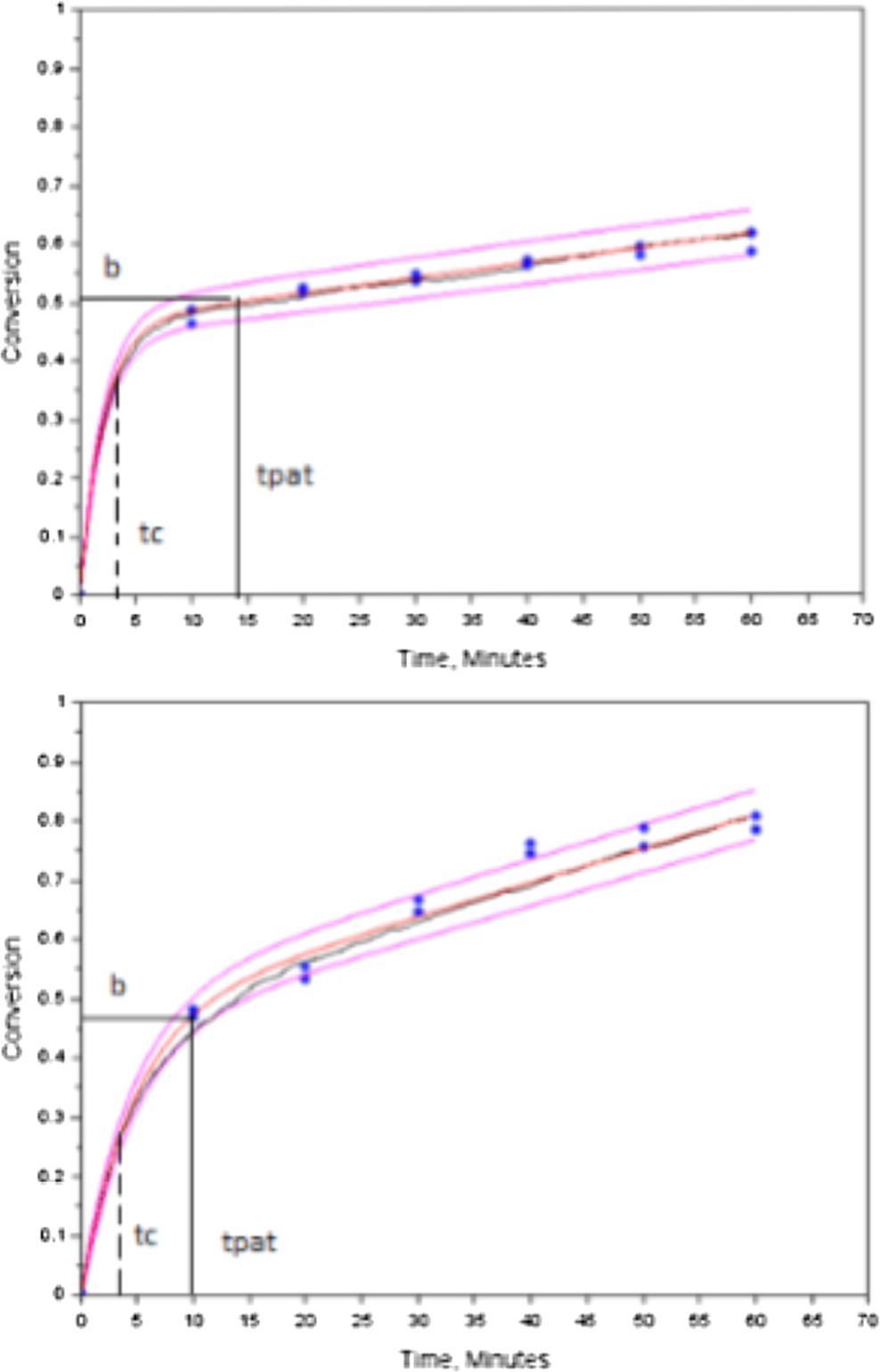
As mentioned, the b parameter value indicates the beginning of the plateau. So, we can estimate the t_c as being the instant when the line y = (b × k) t meets the b plateau value. Therefore, the estimated value for t_c is given by Equation (23). \documentclass{aastex}\usepackage{amsbsy}\usepackage{amsfonts}\usepackage{amssymb}\usepackage{bm}\usepackage{mathrsfs}\usepackage{pifont}\usepackage{stmaryrd}\usepackage{textcomp}\usepackage{portland, xspace}\usepackage{amsmath, amsxtra}\pagestyle{empty}\DeclareMathSizes{10}{9}{7}{6}\begin{document} \begin{align*} { t_c } = \frac { 1 } { k } \tag { 23 } \end{align*} \end{document}

This procedure may be visualized in Fig. 2. In this figure, the initial concentration data until t = 8 min can be approximated to a first-order equation. This value for t is near the proposed one for t_c. At this interval, the mean behavior of the stochastic model also has a good fitting to a linear profile of conversion.

FIG. 2.

Graphic representation of an estimate of initial reaction time where the degradation process (central line) can be adjusted to a linear behavior. External smooth and continue curves represent the prevision of the model. The central smooth and continue curve represents the mean value of the model. The central noise rating curve represents the stochastic simulation. The straight line connecting points on a circle is an approach to the pseudo-first order kinetic equation. The straight line with a +symbol is an approach proposed for the linear behavior based on the model.

So, considering t_c, the mean value of r(t), called Kc₁, integral values divided by t_c can be calculated as shown in Equation (24). \documentclass{aastex}\usepackage{amsbsy}\usepackage{amsfonts}\usepackage{amssymb}\usepackage{bm}\usepackage{mathrsfs}\usepackage{pifont}\usepackage{stmaryrd}\usepackage{textcomp}\usepackage{portland, xspace}\usepackage{amsmath, amsxtra}\pagestyle{empty}\DeclareMathSizes{10}{9}{7}{6}\begin{document} \begin{align*} K { c_1 } = { \frac { \mathop \int \nolimits_0^ { tc } { \frac { \left( { a + { \frac { b \times k } { { e^ { k \times t } } } } } \right) } { 1 - \left( { a \times t + b \left( { 1 - { e^ { - k \times t } } } \right) } \right) } } dt } { { t_c } } } = { \frac { ln \left( { 1 - E \left( { { C_ { tc } } } \right) } \right) } { { t_c } } } \tag { 24 } \end{align*} \end{document}

Where the average value of C_t at the point t_c, E(C_tc), may be given by Equation (25). \documentclass{aastex}\usepackage{amsbsy}\usepackage{amsfonts}\usepackage{amssymb}\usepackage{bm}\usepackage{mathrsfs}\usepackage{pifont}\usepackage{stmaryrd}\usepackage{textcomp}\usepackage{portland, xspace}\usepackage{amsmath, amsxtra}\pagestyle{empty}\DeclareMathSizes{10}{9}{7}{6}\begin{document} \begin{align*} E \left( {{C_{tc}}} \right) = a \times {t_c} + b \left( {1 - {e^{ - k \times {t_c}}}} \right) \tag{25} \end{align*} \end{document}

To estimate Kc₂, we will observe the behavior of E(C_tc) around the tpat. This is because at that instant of time we can have a possible indication of the decreasing reaction rate. In this way, the exponential term for mean concentration of the stochastic model is expanded in a Taylor series around t = tpat, according to Equation (26). \documentclass{aastex}\usepackage{amsbsy}\usepackage{amsfonts}\usepackage{amssymb}\usepackage{bm}\usepackage{mathrsfs}\usepackage{pifont}\usepackage{stmaryrd}\usepackage{textcomp}\usepackage{portland, xspace}\usepackage{amsmath, amsxtra}\pagestyle{empty}\DeclareMathSizes{10}{9}{7}{6}\begin{document} \begin{align*} & E \left( {{C_t}} \right) \approx \\ & \qquad{C_0} \left( {1 - a \times t - b \left( {1 - \left( {{e^{ - k \times tpat}} - k{e^{ - k \times tpat}} \left( {t - tpat} \right) } \right) } \right) } \right) \tag{26}\end{align*} \end{document}

For t = s + tpat, Equation (26) may be written as Equation (27) and rearranged as Equation (28). \documentclass{aastex}\usepackage{amsbsy}\usepackage{amsfonts}\usepackage{amssymb}\usepackage{bm}\usepackage{mathrsfs}\usepackage{pifont}\usepackage{stmaryrd}\usepackage{textcomp}\usepackage{portland, xspace}\usepackage{amsmath, amsxtra}\pagestyle{empty}\DeclareMathSizes{10}{9}{7}{6}\begin{document} \begin{align*} & E \left( {{C_{s + tpat}}} \right) \approx \\ & \qquad{C_0} \left( {1 - a \left( {s + tpat} \right) - b \left( {1 - \left( {{e^{ - k \times tpat}} - k{e^{ - k \times tpat}} \left( s \right) } \right) } \right) } \right) \tag{27}\end{align*} \end{document} \documentclass{aastex}\usepackage{amsbsy}\usepackage{amsfonts}\usepackage{amssymb}\usepackage{bm}\usepackage{mathrsfs}\usepackage{pifont}\usepackage{stmaryrd}\usepackage{textcomp}\usepackage{portland, xspace}\usepackage{amsmath, amsxtra}\pagestyle{empty}\DeclareMathSizes{10}{9}{7}{6}\begin{document} \begin{align*} & E \left( {{C_{s + tpat}}} \right) \approx \\ & \quad{C_0} \left( {1 - a \times tpat - b \left( {1 - {e^{ - k \times tpat}}} \right) - \left( {b \times k{e^{ - k \times tpat}} + a} \right) s} \right) \tag{28}\end{align*} \end{document}

In Equation (28), considering tpat definition, the term a × tpat + b (1−e^−k×tpat) is the value at the beginning of the plateau, that is, the value of parameter b. So, Equation (28) may be approximated by Equations (29) and (30). \documentclass{aastex}\usepackage{amsbsy}\usepackage{amsfonts}\usepackage{amssymb}\usepackage{bm}\usepackage{mathrsfs}\usepackage{pifont}\usepackage{stmaryrd}\usepackage{textcomp}\usepackage{portland, xspace}\usepackage{amsmath, amsxtra}\pagestyle{empty}\DeclareMathSizes{10}{9}{7}{6}\begin{document} \begin{align*} E \left( {{C_{s + tpat}}} \right) \approx {C_0} \left( {1 - b - \left( {b \times k{e^{ - k \times tpat}} + a} \right) s} \right) \tag{29} \end{align*} \end{document} \documentclass{aastex}\usepackage{amsbsy}\usepackage{amsfonts}\usepackage{amssymb}\usepackage{bm}\usepackage{mathrsfs}\usepackage{pifont}\usepackage{stmaryrd}\usepackage{textcomp}\usepackage{portland, xspace}\usepackage{amsmath, amsxtra}\pagestyle{empty}\DeclareMathSizes{10}{9}{7}{6}\begin{document} \begin{align*} E \left( { { C_ { s + tpat } } } \right) \approx { C_0 } \left( { 1 - b } \right) \left( { 1 - { \frac { { \frac { b \times k } { 100 } } + a } { 1 - b } } s } \right) \tag { 30 } \end{align*} \end{document}

Considering \documentclass{aastex}\usepackage{amsbsy}\usepackage{amsfonts}\usepackage{amssymb}\usepackage{bm}\usepackage{mathrsfs}\usepackage{pifont}\usepackage{stmaryrd}\usepackage{textcomp}\usepackage{portland, xspace}\usepackage{amsmath, amsxtra}\pagestyle{empty}\DeclareMathSizes{10}{9}{7}{6}\begin{document} $${C_{tpat}} = {C_0} \left( {1 - b} \right)$$ \end{document} , as the organic load that still has to be converted from instant tpat (thus resetting chronometer), name the organic load that will be transformed from C_tpat into \documentclass{aastex}\usepackage{amsbsy}\usepackage{amsfonts}\usepackage{amssymb}\usepackage{bm}\usepackage{mathrsfs}\usepackage{pifont}\usepackage{stmaryrd}\usepackage{textcomp}\usepackage{portland, xspace}\usepackage{amsmath, amsxtra}\pagestyle{empty}\DeclareMathSizes{10}{9}{7}{6}\begin{document} $$\mathop {{\tilde{C}_s}} = {C_{s + tpat}}$$ \end{document} , which is \documentclass{aastex}\usepackage{amsbsy}\usepackage{amsfonts}\usepackage{amssymb}\usepackage{bm}\usepackage{mathrsfs}\usepackage{pifont}\usepackage{stmaryrd}\usepackage{textcomp}\usepackage{portland, xspace}\usepackage{amsmath, amsxtra}\pagestyle{empty}\DeclareMathSizes{10}{9}{7}{6}\begin{document} $$\mathop {{\tilde{C}_0}} = {C_{tpat}}$$ \end{document} , according to what is used in Equation (31). \documentclass{aastex}\usepackage{amsbsy}\usepackage{amsfonts}\usepackage{amssymb}\usepackage{bm}\usepackage{mathrsfs}\usepackage{pifont}\usepackage{stmaryrd}\usepackage{textcomp}\usepackage{portland, xspace}\usepackage{amsmath, amsxtra}\pagestyle{empty}\DeclareMathSizes{10}{9}{7}{6}\begin{document} \begin{align*} E \left( { \mathop { { { \tilde C } _s } } \limits } \right) \approx { C_ { tpat } } exp \left( { - \left( { { \frac { { \frac { b \times k } { 100 } } + a } { 1 - b } } } \right) \times s } \right) \tag { 31 } \end{align*} \end{document}

An estimate to Kc₂ can be obtained by Equation (32). \documentclass{aastex}\usepackage{amsbsy}\usepackage{amsfonts}\usepackage{amssymb}\usepackage{bm}\usepackage{mathrsfs}\usepackage{pifont}\usepackage{stmaryrd}\usepackage{textcomp}\usepackage{portland, xspace}\usepackage{amsmath, amsxtra}\pagestyle{empty}\DeclareMathSizes{10}{9}{7}{6}\begin{document} \begin{align*} K { c_2 } = { \frac { { \frac { b \times k } { 100 } } + a } { 1 - b } } \tag { 32 } \end{align*} \end{document}

Finally, an estimate of E(C_t) shown in Equation (33) can be considered for times higher than tpat. \documentclass{aastex}\usepackage{amsbsy}\usepackage{amsfonts}\usepackage{amssymb}\usepackage{bm}\usepackage{mathrsfs}\usepackage{pifont}\usepackage{stmaryrd}\usepackage{textcomp}\usepackage{portland, xspace}\usepackage{amsmath, amsxtra}\pagestyle{empty}\DeclareMathSizes{10}{9}{7}{6}\begin{document} \begin{align*} & E \left( {{C_t}} \right) = {C_0} \left( {1 - E \left( {{X_t}} \right) } \right) = \\ & \qquad{C_0} \left( {1 - a \times t - b \left( {1 - exp \left( { - k \times t} \right) } \right) } \right) \approx {C_0} \left( {1 - b - a \times t} \right) \tag{33}\end{align*} \end{document}

On the contrary, when time is longer than tpat, E(C_t) may be obtained by Equation (34). \documentclass{aastex}\usepackage{amsbsy}\usepackage{amsfonts}\usepackage{amssymb}\usepackage{bm}\usepackage{mathrsfs}\usepackage{pifont}\usepackage{stmaryrd}\usepackage{textcomp}\usepackage{portland, xspace}\usepackage{amsmath, amsxtra}\pagestyle{empty}\DeclareMathSizes{10}{9}{7}{6}\begin{document} \begin{align*} \begin{split}E \left( {{C_t}} \right) & \approx {C_0} \left( {1 - b} \right) - {C_0} \left( {1 - b} \right) \left( {{a \over {1 - b}}} \right) t \\& \approx {C_{tpat}} - {C_{tpat}}{a \over {1 - b}}t\end{split} \tag{34}\end{align*} \end{document}

Equation (34) may be compared to the conversion of a zero-order reaction. It is possible to estimate the time necessary for total initial load degradation, called t1, in Equation (35). \documentclass{aastex}\usepackage{amsbsy}\usepackage{amsfonts}\usepackage{amssymb}\usepackage{bm}\usepackage{mathrsfs}\usepackage{pifont}\usepackage{stmaryrd}\usepackage{textcomp}\usepackage{portland, xspace}\usepackage{amsmath, amsxtra}\pagestyle{empty}\DeclareMathSizes{10}{9}{7}{6}\begin{document} \begin{align*} t1 = \frac { { 1 - b } } { a } \tag { 35 } \end{align*} \end{document}

Experimental Protocols

Effluents

Three different effluents were used in this work. Two of them are real effluents: from a leachate and a dairy industry. In this work, we propose to compare, when possible, kinetic constants estimated by the model, Kc₁ and Kc₂ (Method I) with those calculated by first-order kinetic equations, kc₁ and kc₂ (Method II). In the case of the leachate, the experimental data allow to separate, although in a somewhat arbitrary way, TOC conversion in two phases with different kinetic constants. For benzoic acid, we used the estimates provided by Chen et al. (2011). To the dairy effluent, no experimental data were obtained in the fast phase conversion. So, it was impossible to estimate the constant kinetic for the first phase, Kc₁. However, using the methodology proposed in this article, it is possible to estimate this constant.

Leachate was provided by VSA—Vale Soluções Ambientais Company, located in the city of Cachoeira Paulista, São Paulo, Brazil. Leachate samples were taken from passing box, from a simple and punctual source. In March 2015, 300 L of leachate was collected from the sanitary landfill to be conducted through all steps of this project. After that, effluent volume was homogenized by mechanical agitation and split on plastic drums of 50 L each and kept at 4°C. The time of leachate sampling was characterized by a low pluviometric index that did not influence directly the characteristics of leachate produced by landfill previously specified. There are no protocols for sampling, filtration, and stocking of leachate samples (Kjeldsen et al., 2002). Therefore, recommendations for preserving samples from sanitary wastewater were applied. Other studies and practice show that leachate samples are not easily degraded as sanitary wastewater samples. To each experiment performed, the required samples were collected and kept at room temperature on the same day of experiment, minimizing possible physical changes to the samples. Leachate samples collected from Sanitary Landfill of VSA–Vale Soluções Ambientais Company, have a pH of 8.5 ± 0.1. Values higher than 8.0 are characteristics of leachate in advanced stages of organic matter. This fact is interesting because the cell worked in this landfill was still receiving residues. Physical–chemical characteristics of leachate in natura are given by the following parameters: COD 3,457 mg O₂/L, TOC 1,130 mg C/L, BOD₅ 225 mg O₂/L, N-NH₃ 1,250 mg/L, total solids 10,398 mg/L, oil and fats 805 mg/L, and phenol 118 mg/L. The ratio BOD/COD is shown to be lower than 0.2, which classifies it as nonbiodegradable. More details of this procedure and characteristics can be found in Almeida et al. (2009).

Leachate was treated by AOP (catalytic ozonation). Three experimental conditions were selected, here denoted as A1, A2, and A3. In condition A1: 0.5 L O₃/min, 0.35 g/[Fe²⁺·L], and pH = 6. In condition A2: 0.25 L O₃/min, 0.5 g/[Fe²⁺·L], and pH = 3. In condition A3: 0.75 L O₃/min, 0.2 g/[Fe²⁺ L], and pH = 3.

Figure 3 presents a detailed scheme of AOP treatment for the leachate effluent. The oxidation process of the organic matter happens in the reactor (1). It contains a cylinder shape in all its extension. This reactor has the input of O₂ + O₃ (4), from the ozonator (6), introduction of the catalytic solution (7), effluent feeding (9), and sampling (11). O₂ + O₃ input is carried out by the base of the reactor (4) as microbubbles, using a porous stone from fish tanks (4a) for better adsorption of O₂ + O₃ and homogenization of oxidative system. The flow is upward in which oxygen cylinder (5) of O₂ (or an air centrifuge pump) is transformed in ozone by an electric discharge method that happens in the ozonator (6). Catalytic solution is fed (7) at 17 cm above O₂ + O₃ inlet, although at the opposite side. Solution (7a) is previously prepared in sulfuric media and introduced to the reactor by a peristaltic pump (8), which is added 10 s after the ozone input and remains 20 min of total reaction time, which is 30 min. Effluent recycle is fed after foam is broken at the entry of the reactor (9) by means of pulse pump (10). Sampling (11) is carried out manually through a glass valve open/close type that allows sampling fast and close to the system without interfering with it. Module (2) is shaped as a cone and attached to the reactor by a metallic clip (2a). It consists of a glass tube (2b) curved at 180°. This tube contains a needle in its interior (2c) projected to favor the flow, where atmospheric air is introduced by a centrifuge pump with the function of breaking superficial tension of foam (2d), whose outlet allows the attachment of a hose (2e) to the transferring of effluent to third module (3) (reservoir) connected to a pulse pump (10). This pumps liquid back to the entry of the system (9) as a recycle, not compromising the volume and reactional kinetics completing the cycle of configuration of reactor.

FIG. 3.

Layout of experimental procedure on bench-scale of the AOP treatment step for the leachate.

Literature was used in the synthetic effluent (benzoic acid) treated by AOP (Fenton + hydroxylamine). Data used were based on Chen et al. (2011), whose study monitored the conversion of Fe(III) and Fe(II) during the treatment.

Another effluent used in this study came from a dairy industry located in the city of Guaratinguetá, region of Vale do Paraíba in the State of São Paulo, Brazil. Details on sampling, collecting, preservation, and characteristics of the effluent may be found in Loures et al. (2014). Dairy effluents have a great amount of lipids, carbohydrates, and proteins giving the system a high organic load. They have high COD and BOD₅. It is common to find values up to 10,000 and 2.50 mg/L for COD and BOD₅, respectively. In addition, a DBO₅/COD ratio of about 0.25 was found for this respective effluent.

The dairy effluent was treated by photo-Fenton, considering different levels of pH, Fenton reagent (Fe²⁺ + H₂O₂), and UV radiation. In this study, we selected two conditions to modeling. In condition B1, pH = 3.5; Fe²⁺/H₂O₂ = 12.5; UV = 15 W; in condition B2: pH = 4.0; Fe²⁺/H₂O₂ = 12.5; UV = 0 W.

Figure 4 presents the detailed scheme of AOP treatment for the dairy industry effluent. The photochemical treatment was carried out with a constant feeding batch. Details on the steps of the photo-Fenton process for this effluent are found in Loures et al. (2014).

FIG. 4.

Layout of experimental procedure on bench-scale of the AOP treatment step for the dairy effluent.

Results and Discussion

Leachate effluent

The adjustment of the model for the leachate effluent considering three experimental conditions previously mentioned (A1, A2, and A3) is presented in Fig. 5. In this figure, it is possible to notice a good adjustment of the model to do the experimental data, considering the three studied experimental conditions. In addition, it was evidenced that there were two different conversion rates for the effluent. Another interesting observation concerns about the CI width. This width changes according to the global behavior of the experimental data in each condition.

FIG. 5.

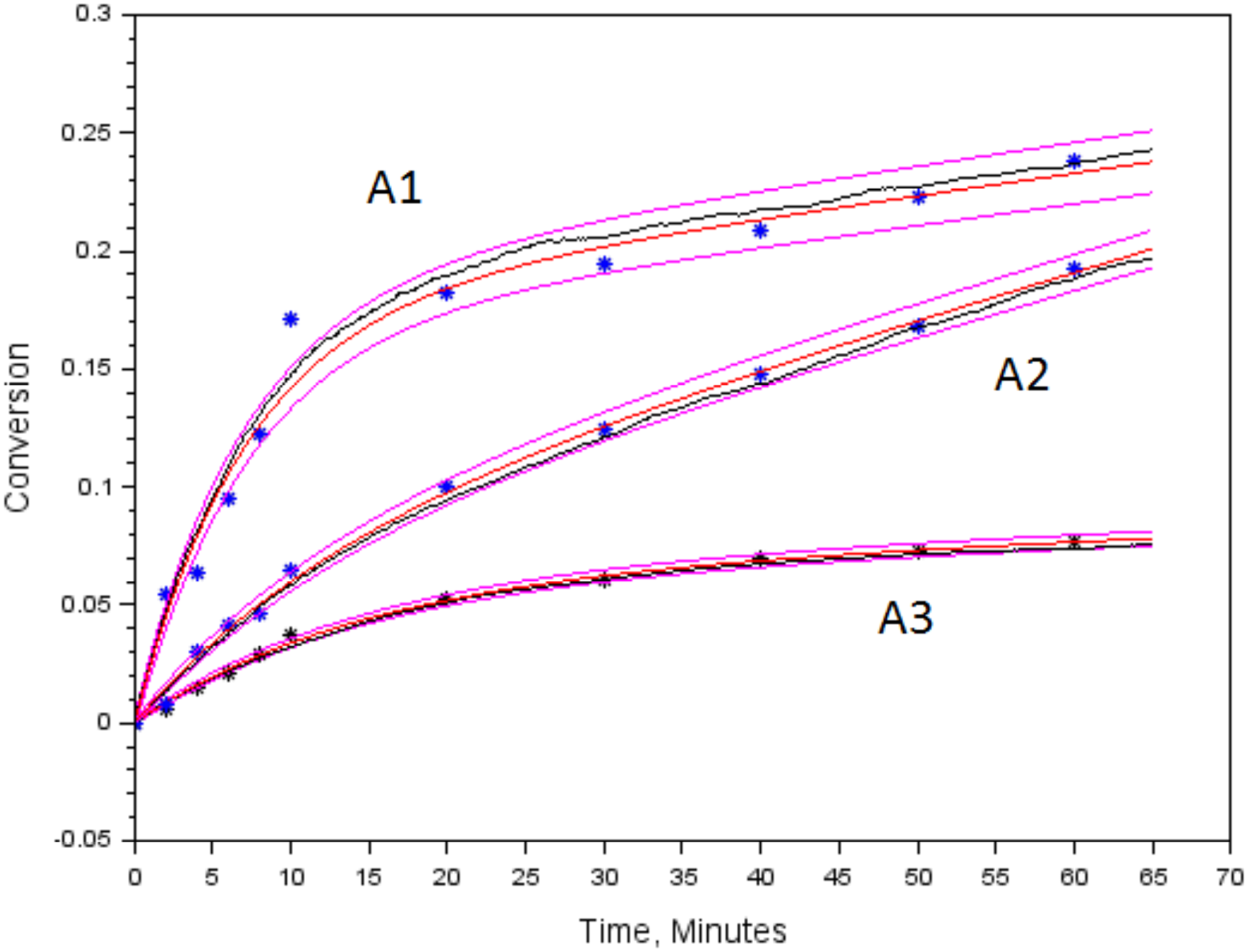
TOC conversion for leachate effluent considering different experimental conditions. A1: 0.5 L O₃ min⁻¹, 0.35 g Fe²⁺ L⁻¹, pH = 6. A2: 0.25 L O₃ min⁻¹, 0.5 g Fe²⁺ L⁻¹ and pH = 3. A3: 0.75 L O₃ min⁻¹, 0.2 g Fe²⁺ L⁻¹ and pH = 3. Smooth continuous lines represent average values and confidence interval predicted by the model. The central noise black lines represent a model prediction considering studied experimental conditions (A1, A2 and A3). The symbol “*” represent experimental data.

The adjusted model parameters found for this effluent are shown in Table 1. The high values for R² (higher than 0.98) show that the predicted model of mean behavior of experimental data fits well to experimental data. Moreover, Fig. 5 shows a numerical simulation of stochastic model [Equation (1)] to each experimental condition (A1, A2, and A3). Results showed a good fit of model to describe different experimental conditions.

Table 1.

Model-Predicted Parameters for Leachate Considering Three Experimental Conditions (A1, A2, and A3)

	Experimental Conditions
Parameters	A1	A2	A3
a	0.00095 ± 0.00055	0.00197 ± 0.00020	0.00025 ± 0.00010
b	0.17580 ± 0.02098	0.07305 ± 0.00869	0.06233 ± 0.00454
c	0.00245 ± 0.00018	0.00090 ± 0.00004	0.00053 ± 0.00001
k	0.14 ± 0.01006	0.08 ± 0.01725	0.07 ± 0.00681
p	0.37 ± 0.00058	0.19 ± 0.00094	0.35 ± 0.00088
R ²	0.97777	0.99752	0.99689
t_c (minute)	7.14	12.5	14.5
tpat (minute)	17.04	13.05	30.17
t1 (hour)	14.3	7.8	61

A1, 0.5 L O₃/min, 0.35 g/[Fe²⁺ L], and pH = 6; A2, 0.25 L O₃/min, 0.5 g/[Fe²⁺·L], and pH = 3; A3, 0.75 L O₃/min, 0.2 g/[Fe²⁺·L], and pH = 3. The tpat was estimated by Equation (5).

It is possible to see that leachate degradation data shown in Fig. 5 may be understood with the aid of stochastic model parameters, presented in Table 1. First, the b parameter marks the beginning of the degradation plateau. The values for b parameter are consistent with the values shown in the figure. When the values for t_c are observed, in all the experimental conditions (A1, A2, and A3), it is possible to notice a linear behavior of the experimental data for t < t_c. The values for t_c (Table 1) were 7, 12, and 14 min for A1, A2, and A3, respectively. In this time intervals, both model predicted and experimental data showed a linear tendency. It is consistent with an approximation of a pseudo-first-order reaction for TOC conversion.

Identifying when the plateau of conversion begins is a difficult task for some experimental conditions. The b parameter gives an estimative for the time necessary to reach the plateau (tpat). In Table 1, the values for b and tpat are indicated. Visually, this approximation seems to be reasonable with the curves of Fig. 5.

As already mentioned, the a parameter is related to the plateau slope. The slope of the plateau will define the necessary time to complete reaction (t1). A greater plateau slope indicates a minor time for maximum organic load conversion. This time may be calculated here according to Equation (24). Conversion curves shown in Fig. 5 show that the reaction in condition A2 will be faster than A1 and A3, which is in accordance with estimates of the a parameter and t1.

The c and p parameters are related to the width of the CI. The c parameter for A3 experimental condition is about five times less than for A1. This represents a much narrower CI for A3 experimental conditions than for A1. This behavior may also be evidenced in Fig. 5. For A2, the CI width presented an intermediary behavior between A1 and A3.

Table 2 shows kinetic parameters (Kc₁ and Kc₂) predicted by the model (Method I) and the calculated by a first-order equation approximation (kc₁ and kc₂, Method II).

Table 2.

Kinetics Parameters Predicted by the Model and by First-Order Equation for Leachate Effluent Under Three Experimental Conditions (A1, A2, and A3)

	Experimental Conditions
Method	A1	A2	A3
Method I
Kc₁ (s⁻¹)	0.01757 ± 0.00191	0.00588 ± 0.00059	0.00308 ± 0.00012
Kc₂ (s⁻¹)	0.0015 ± 0.0004	0.0022 ± 0.0003	0.0003 ± 0.0002
Method II
Kc₁ (s⁻¹)	0.01707	0.00660	0.00378
Kc₂ (s⁻¹)	0.00176	0.00269	0.00066

Method I: calculated directly from the stochastic model. Method II: calculated from the first-order kinetic equation approximation. A1, 0.5 L O₃/min, 0.35 g/[Fe²⁺·L], and pH = 6; A2, 0.25 L O₃/min, 0.5 g/[Fe²⁺ L], and pH = 3; A3, 0.75 L O₃/min, 0.2 g/[Fe²⁺ L], and pH = 3.

According to data from Table 2, two steps of different conversion can be seen: a fast initial and a slow one afterward. This behavior goes accordingly to what authors (Orbeci et al., 2014; Chen et al., 2011) observed. It is important to point out that predicted values to the stochastic model of Kc₁ and Kc₂ are close to the ones obtained by first-order kinetic equation. It is worth noticing that to calculate kc₁ and kc₂ from the kinetic equation, it is necessary that experimental data show a favorable kinetic profile to the division in two phases. In addition, as shown here and in other work, the duration of the first phase can be extremely fast making it difficult to obtain intermediate experimental data during this stage. Under this situation, the proposed methodology in this work would make it easy to estimate kinetic parameters.

Synthetic effluent (Benzoic Acid)

This effluent was treated by AOP (Fenton) combined with the use of hydroxylamine by Chen et al. (2011). Same comments in relation to quality of adjustment of the model to experimental data done to leachate were also applied to the synthetic effluent analyzed here (Table 3).

Table 3.

Model-Predicted Parameters for Synthetic Effluent

Parameters	Values
a	0.00950 ± 0.00130
B	0.18404 ± 0.00820
C	0.00778 ± 0.00042
K	1.28 ± 0.30201
P	1. ± 0.00740
R ²	0.99781
t_c (minute)	0.78
tpat (minute)	1.84
t1 (hour)	1

Those authors presented a table with estimates to kinetic constants of pseudo-first order to the two phases, kc₁ and kc₂ (Table 4). Data were digitalized and in terms of comparison, the stochastic model was adjusted and kinetic constants estimated by methodology presented in this article. Data from Table 4 show that estimates are similar to kinetic constants provided by the application of model and by equations of first order.

Table 4.

Kinetics Parameters Predicted by the Model and by First-Order Equation for Benzoic Acid Synthetic Effluent

Method	Constant	Values
Method I	Kc₁ (s⁻¹)	0.16911 ± 0.03707
	Kc₂ (s⁻¹)	0.015 ± 0.006
Method II	Kc₁ (s⁻¹)	0.151
	Kc₂ (s⁻¹)	0.016

Method I: calculated directly from the stochastic model. Method II: calculated from the first-order kinetic equation approximation by Chen et al. (2011).

Dairy industry effluent

In relation to conversion data to the dairy effluent (Table 5), a good adjustment is found between estimates of model and experimental data (R² higher than 0.98). Same comments in relation to the quality of the adjustment of model to experimental data conducted to other effluents are also applicable to the dairy effluent analyzed. A point worth noticing is that replicates were performed for each studied condition. In Fig. 6, it is possible to realize that the vast majority of replicates from experimental data are within the delimited range of confidence level predicted by the model.

FIG. 6.

TOC conversion for dairy industry effluent. Condition B1: pH = 3.5; Fe²⁺/H₂O₂ = 12.5; UV = 15 W. Condition B2: pH = 4.0; Fe²⁺/H₂O₂ = 12.5; UV = 0 W. Smooth continuous lines represent average values and confidence interval predicted by the model. The central noise black lines represent a model prediction considering studied experimental conditions (B1 and B2). The symbol “*” represent experimental data.

Table 5.

Model-Predicted Parameters for the Dairy Industry Effluent Considering Two Experimental Conditions (B1 and B2)

	Experimental Conditions
Parameters	B1	B2
A	0.00141 ± 0.00012	0.00574 ± 0.00159
B	0.50542 ± 0.00492	0.46657 ± 0.06335
C	0.00874 ± 0.00039	0.00926 ± 0.00082
K	0.22 ± 0.03971	0.22 ± 0.04329
P	0.47 ± 0.00091	0.44 ± 0.00002
R ²	0.99988	0.98864
t_c (minute)	4.54	4.54
tpat (minute)	14.46	9.67
t1 (hour)	3.5	1.6

Condition B1: pH = 3.5; Fe²⁺/H₂O₂ = 12.5; UV = 15 W. Condition B2: pH = 4.0; Fe²⁺/H₂O₂ = 12.5; UV = 0 W. The tpat was estimated by Equation (5).

Experimental data were not obtained during the fast conversion phase of this effluent. This made it hard to estimate the kinetic constant (Kc₁) for this phase. However, based on the proposed methodology of this article, it was possible to obtain an estimate to this constant (Table 6).

Table 6.

Kinetics Parameters Predicted by the Model and by First-Order Equation for Dairy Industry Effluent Under Two Experimental Conditions (B1 and B2)

		Experimental conditions
Method	Constant	B1	B2
Method I	Kc₁ (s⁻¹)	0.08675 ± 0.0117555	0.08518 ± 0.02687
	Kc₂ (s⁻¹)	0.005 ± 0.002	0.013 ± 0.003
Method II	Kc₁ (s⁻¹)	^*	^*
	Kc₂ (s⁻¹)	0.00588	0.01905

Method I: calculated directly from the stochastic model. Method II: calculated from the first-order kinetic equation. ^*: For Method II, the K₁ was not calculated from the first-order kinetic equation, due to the lack of experimental points in the rapid initial phase of the conversion. Condition B1: pH = 3.5; Fe²⁺/H₂O₂ = 12.5; UV = 15 W. Condition B2: pH = 4.0; Fe²⁺/H₂O₂ = 12.5; UV = 0 W.

Model validation

To obtain more evidence for the model validation, it is possible to evaluate the probability of each experimental point that has been generated by the model. Hence, the pseudo-residual technique described in Zucchini and MacDonald (2009) may be used for the evaluation model. This technique was used here only for the dairy effluent, since a great number of experimental data were available. The idea of this technique is that if the model is correct then the inverse function of the accumulated probability of experimental points follows a uniform distribution. Represented in symbols, u_t = P (X_t ≤ x_t), u_t uniform. However, instead of testing the hypothesis of u_t being distributed uniformly (Zucchini and MacDonald, 2009), it is recommended to transform u_t in a normal standard distribution and then proceed with the tests so that the hypothesis of the transformed variable follows the normal standard, Z_t = Φ⁻¹ (u_t), where Φ is the normal standard distributed function. The transformed variable Z_t is called normal pseudo-residual. Thus, the Z_t variable was calculated for every experimental point, and the hypothesis of normality was tested as shown in Fig. 7.

FIG. 7.

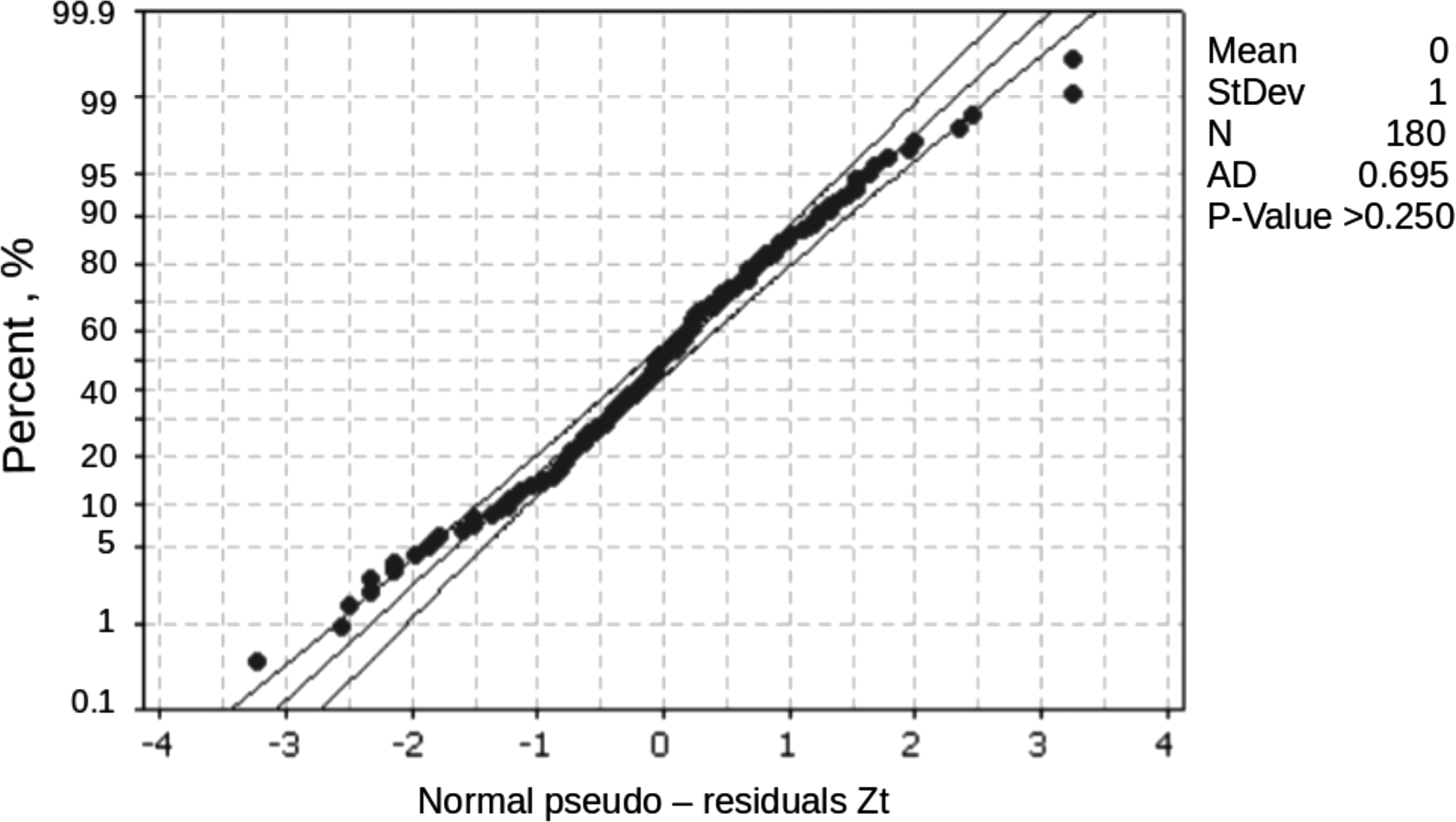
Probability plot of Z_t.variable considering dairy effluent experimental data (Normal – 95%).

Based on the statistics of Anderson–Darling, (p > 0.250), the results fail to reject that Z_t follows a normal distribution. Thus, based on the analyzed sample, the hypothesis that the stochastic model proposed is adequate to describe the variations of the process of degradation via AOP and cannot be rejected in the experimental conditions studied.

Model relevance

The stochastic nature of the model creates CI for both experimental measurements and for the model parameters. As degradation has generally a nonlinear behavior, the computer simulation of the stochastic model provides a simple alternative in estimating these CIs. To studying oxidation at various stages, the averaged behavior of the model was used, as described. The averaged behavior is not stochastic, it is only a function of time when the model parameters are known.

In addition, to develop mechanisms and study reaction order, synthetic samples are used, as found in the literature. This is unlike the complex samples with different organic families found in industrial waste. Industrial effluents with complex and distinct physical and chemical properties were used. This renders difficulties in the kinetic study due to differentiated oxidation behaviors resulting from the amount and type of carbon involved in the reactions. Despite the complexity of these reactions, the model properly simulated degradation even when there was minimal or no data point in the initial phase.

Conclusions

The stochastic model may significantly describe the TOC conversion profile for natural effluents (leachate, dairy) and synthetic one (benzoic acid) treated by AOP that have chemically different mechanisms concerning formation of hydroxyl radicals.

It is possible to describe the average behavior and experimental data variability, even that the specific chemical reactions involved in the organic carbon degradation are not known. This is an advantage when working with natural effluents, since it is difficult to analyze all the reactions involved in the process.

Conversion of the studied effluents follows a two-phase behavior: a rapid initial phase followed by a slower one, which may be described concomitantly by the model.

With model parameters, it is possible to obtain approximations for the initial time interval where a pseudo-first-order reaction can be approximate (t_c). It is also possible to obtain the instant when the degradation process initiates a slower conversion phase (time to reach the plateau, tpat).

The methodology here developed allows to estimate the kinetic constants for the TOC conversion initial fast phase as well for the slower phase. Those constants are similar to the traditional kinetic equations calculated. This may be an alternative when the initial conversion phase is very fast, making difficult to obtain experimental data in a short period of time.

In a more comprehensive way, the proposed stochastic model evidences that, independently of the effluent organic function and its chemical composition, it is possible to express the degradation kinetic profile as a function of the TOC variable.

Footnotes

Acknowledgments

The authors thank Cia de Alimentos Glória, city of Guaratinguetá, State of São Paulo, Brazil, for the dairy effluent sample provided for this work as well as the laboratories used in the development of this study. They also thank VSA—Vale Soluções Ambientais Company, State of São Paulo, for kindly providing the leachate. They also thank the Coordinating Agency for Advanced Training of Graduate Personnel (Coordenação de Aperfeiçoamento de Pessoal de Nível Superior—CAPES) for financial support to this Master's study. To FAPESP Process 2009/17650-2.

Author Disclosure Statement

No competing financial interests exist.

Nomenclature

References

Almeida

, Assalin

M.R.

, Rosa

M.A.

, and Durán

(2004). Tratamento de efluentes industriais por processos oxidativos avançados na presença de ozônio. Quím. Nova., 27, 818.

Almeida

, Lima

E.N.

, Crespi

M.S.

, Ribeiro

C.A.

, and Schalch

(2009). Kinetic studies of urban solid residues and leachate from sanitary landfill. J. Therm. Anal. Calorim., 97, 529.

Banu

J.R.

, Anadan

, Kaliappan

, and Yeom

I.T.

(2008). Treatment of dairy wastewater using anerobic and solar photocatalytic methods. Sol. Energy., 82, 812.

Baun

, Ledin

, Reitzel

L.A.

, Bjerg

P.L.

, and Christensen

T.H.

(2004). Xenobiotic organic compounds in leachates from ten Danish MSW landfills: Chemical analysis and toxicity tests. Water Res. 38, 3845.

Chen

, Ma

, Li

, Zhang

, Fang

, Guan

and Xie

(2011). Strong enhancement on Fenton oxidation by addition of hydroxylamine to accelerate the ferric and ferrous iron cycles. Environ. Sci. Technol., 45, 3925.

Cordi

, Assalin

M.R.

, Diez

M.C.

, and Duran

(2008). Montagem, partida e operação de um sistema de lodos ativados para o tratamento de efluentes: Parâmetros físico-químicos e biológicos. Eng. Amb., 5, 97.

Efron

, and Tibshirani

R.J.

(1993). An Introduction to the Bootstrap. New York: Chapman & Hall/CRC.

Gavala

H.N.

, Kopsinis

, Skiadas

I.V.

, Stamatelatou

, and Lyberatos

(1999). Treatment of dairy wastewater using an upflow anaerobic sludge blanket reactor. J. Agric. Eng. Res., 73, 59.

Hwu

C.-S.

, Tseng

S.-K.

, Yuan

C.-Y.

, Kulik

, and Lettinga

(1998). Biosorption of long-chain fatty acids in UASB treatment process. Water Res., 32, 1571.

10.

International Energy Agency (IEA). (2011). World Energy Outlook. Paris: Organisation for Economic Co-operation and Development. Available at: www.iea.org/publications/freepublications/publication/weo2011_web.pdf Accessed December 1, 2011.

11.

Kelly

, Platen

, and Sørensen

(2004). Estimation for discretely observed diffusions using transform functions. J. Appl. Probab., 41, 99.

12.

Kjeldsen

, Barlaz

M.A.

, Rooker

A.P.

, Baun

, Ledin

, and Christensen

(2002). Present and long-term composition of MSW landfill leachate: A review. Environ. Sci. Technol., 32, 297.

13.

Loures

C.C.A.

, Alcântara

M.A.K.

, Izário Filho

H.J.

, Teixeira

A.C.S.

, Silva

F.T.

, Paiva

T.C.B.

, and Lamas-Samanamud

G.R.

(2013). Advanced oxidative degradation processes: Fundamentals and applications. I. Rev. Chem. Eng., 5, 102.

14.

Loures

C.C.A.

, Izário Filho

H.J.

, Oliveira

I.S.

, Lamas-Samanamud

G.R.

, Souza

A.L.

, and Silva

M.B.

(2014). The application of response surface methodology in the study of photodegraded industrial dairy effluents by the photo-Fenton process: Optimization and economic viability. ISRN Chem. Eng., 2014, 1.

15.

Malato

, Blanco

, Fernandez-Alba

A.R.

, and Aguera

(2000). Solar photocatalytic mineralization of commercial pesticides: Acrinathrin. Chemosphere. 40, 403.

16.

Orbeci

, Untea

, Nechifor

, Segneanu

A.E.

, and Craciun

M.E.

(2014). Effect of a modified photo-fenton procedure on the oxidative degradation of antibiotics in aqueous solutions. Sep. Purif. Technol., 122, 290.

17.

Pan

S.H.

, Lo

K.V.

, Liao

P.H.

, and Schreier

(2006). Microwave pretreatment for enhancement of phosphorus release from dairy manure. J. Environ. Sci. Health B., 41, 451.

18.

Pupo Nogueira

R.F.

, Trovo

A.G.

, Silva

M.R.A.

, and Villa

R.D.

(2007). Fundamentos e aplicações dos processos Fenton e foto-Fenton. Quím. Nova., 30, 400.

19.

Rey

, Faraldos

, Casas

J.A.

, Zazo

J.A.

, Bahamonde

, and Rodryguez

J.J.

(2009). Catalytic wet peroxide oxidation of phenol over Fe/AC catalysts: Influence of iron precursor and activated carbon surface. Appl. Catal. B-Environ., 86, 69.

20.

Salazar

R.F.S.

, and Izário Filho

H.J.

(2009). Aplicação de processo oxidativo avançado baseado em fotocatálise heterogênea (TiO₂/UVsolar) para o pré-tratamento de afluente lácteo. Augmdomus. 1, 27.

21.

Siqueira

A.F.

, Guimarães

O.L.C.

, Izario Filho

H.J.

, Giordani

D.S.

, Oliveira

I.S.

, Aquino

H.O.Q.

, and Silva

M.B.A.

(2013). Modeling the photocatalytic process of variation in chemical oxygen demand via stochastic differential equations. Open Chem. Eng. J., 7, 1.

22.

Villa

R.D.

, Silva

M.R.A.

, and Nogueira

R.F.P.

(2007). Potencial de aplicação do processo foto-Fenton/solar como pré-tratamento de efluente da indústria de laticínios. Quím. Nova., 30, 1799.

23.

Zucchini

, and MacDonald

I.L.

(2009). Hidden Markov Models for Time Series: An Introducing Using R. Boca Raton: Chapman and Hall/CRC.