Application of Classification Trees for Predicting Disinfection By-Product Formation Targets from Source Water Characteristics

Abstract

Formation and speciation of disinfection by-products (DBPs) depend on source water constituents. Many studies have sought to model the formation of DBPs using both source water and in-plant operational data, and although sometimes highly predictive of DBP formation, these models are limited in their applicability. To create regional models that could apply to multiple plants within a watershed, classification trees were used to predict finished water DBP parameters from source water constituents collected at multiple locations in a watershed. Data were from a field study conducted in the Monongahela River in southwestern PA from May, 2010 to September, 2012, incorporating six different sites. Classification trees were used to predict violation of, or compliance with, four threshold values that have regulatory and operational significance, namely, the total trihalomethanes (TTHMs) maximum contaminant level (MCL) (regulatory standard of 80 μg/L), 80% of the TTHMs MCL (64 μg/L), a bromine incorporation factor of 0.75, and 50% brominated THMs by mass. The classification trees demonstrated accuracies of 76–83%. Fluorescence measurements were selected in all classification trees, demonstrating their utility in DBP predictive models. Furthermore, model validation using data from each collection site demonstrated the potential use of classification models across this spatially variable region for drinking water plants unable to collect their own source water data. Thus, classification trees provide a valuable tool for creating watershed-level source water-based DBP models.

Introduction

Drinking water disinfection protects consumers from waterborne pathogens; however, it contributes to the formation of harmful disinfection by-products (DBPs). DBPs form when natural organic matter (NOM), found in natural waters, is oxidized by disinfectants necessary for control of pathogenic microorganisms. The highly complex and variable NOM present in water poses a challenge for drinking water treatment because the nature of the NOM affects the speciation as well as the extent of DBP formation (Reckhow et al., 1990; Kitis et al., 2002; Singer et al., 2002; Liang and Singer, 2003; Abouleish and Wells, 2015).

DBP formation is further complicated by the presence of other ions in the source water (Singer and Chang, 1989), most notably bromide. Source water bromide leads to increased formation of DBPs, among them brominated DBP species (Richardson et al., 2003; Navalon et al., 2008; Chowdhury et al., 2010; Watson et al., 2015), which are more toxic than the chlorinated forms (Plewa et al., 2002; Richardson et al., 2003, 2007). DBP exposure, through ingestion of drinking water or inhalation of compounds volatilized during indoor use of disinfected water, has been linked to adverse health effects, such as bladder cancer (King and Marrett, 1996; Villanueva et al., 2004; Cantor et al., 2010; Danileviciute et al., 2012; Kumar et al., 2014). To protect public health, certain classes of DBPs are regulated by the U.S. Environmental Protection Agency (EPA, 2006).

High observed variability of DBP formation and speciation in drinking water has been the subject of extensive research. Differences in the type of disinfectant used are responsible for some of the differences observed in DBP speciation (Hua and Reckhow, 2007b; Montesinos and Gallego, 2013; Pisarenko et al., 2013; Tian et al., 2013; Mao et al., 2014). In addition, seasonal changes in temperature and chlorine demand, oxidant reaction time, and water residence time within the distribution system, all affect DBP formation (Chen and Weisel, 1998; Rodriguez et al., 2004, 2007; Sohn et al., 2006; Hua and Reckhow, 2012; Allard et al., 2015; Sakai et al., 2015). Furthermore, the variability in NOM, particularly the humic/fulvic content, the aromaticity, and the hydrophobic and hydrophilic fractions, has been linked to variability in DBP formation and speciation (Reckhow et al., 1990; Kitis et al., 2002; Singer et al., 2002; Liang and Singer, 2003; Hua and Reckhow, 2007a; Lu et al., 2009).

Since DBP formation and speciation are dependent on the nature of the organic matter present in the source water, multiple methods for quantifying and characterizing NOM have been assessed, including total organic carbon (TOC), dissolved organic carbon (DOC), and ultraviolet absorbance at 254 nm (UV₂₅₄) (Amy et al., 1987; Harrington et al., 1992; Korn et al., 2002; Weishaar et al., 2003; Sohn et al., 2004; Chen and Westerhoff, 2010; Abouleish and Wells, 2015; Awad et al., 2016).

A composite term, SUVA₂₅₄ (UV absorbance normalized by DOC), is frequently used in DBP studies (Edzwald et al., 1985; Kitis et al., 2002; Hua et al., 2015) because it has been shown to be a good indicator of chlorinated DBP formation (Kitis et al., 2001; Li et al., 2014a; Mayer et al., 2015), and in some cases better than TOC in treatment plant operational control (Najm et al., 1994). However, UV₂₅₄ and SUVA₂₅₄ may be less useful for DBP formation and speciation prediction when NOM is of low molecular weight and low aromaticity (Ates et al., 2007; Li et al., 2014a). Although SUVA₂₅₄ may be predictive of certain classes of DBPs, in some data sets, it has also shown weak correlations with trihalomethanes (THMs), a commonly observed and regulated class of DBPs (Hua et al., 2015).

Excitation–emission matrices (EEMs) are gaining attention as an improved method for predicting DBP formation because they provide a large amount of data to capture the complexity and heterogeneity of NOM (Stedmon et al., 2003; Stedmon and Markager, 2005; Baghoth et al., 2011; Pifer et al., 2011; Pifer and Fairey, 2012; Awad et al., 2016). Differential absorbance and fluorescence and differential log-transformed absorbance and fluorescence have shown promise as DBP predictive tools, as studies have shown high correlations between these NOM measurements and multiple DBP species (Roccaro et al., 2008, 2009; Roccaro and Vagliasindi, 2010; He et al., 2015).

To convert EEMs for further analysis and use in predictive models, while incorporating all the data obtained from EEMs, parallel factor analysis (PARAFAC) is often used because it simplifies large, multidimensional data into a few representative components, similar to principal component analysis (Harshman and Lundy, 1994; Stedmon and Markager, 2005; Murphy et al., 2013). Studies have shown promise for the use of EEM–PARAFAC components in predicting DBP formation (Johnstone et al., 2009; Pifer and Fairey, 2014; Sakai et al., 2015; Yang et al., 2015a, 2015b). Furthermore, research by Pifer and Fairey (2012) on EEMs coupled with PARAFAC has demonstrated that EEM–PARAFAC components may be better at predicting DBP formation than SUVA₂₅₄. Other research has illustrated the unique ability of EEM–PARAFAC components to differentiate NOM among sources when using sampling from multiple sites (Cabaniss and Shuman, 1987; Sierra et al., 1994; He and Hur, 2015).

Pifer and Fairey's (2014) success in developing strong correlations between EEM–PARAFAC components and DBP formation potential of natural raw water samples chlorinated and measured in the laboratory provides motivation for using similar NOM characterizations for predicting DBP formation in full-scale treatment plants across a watershed. Assessing treatability using fluorescence EEM–PARAFAC components remains a challenge, however, as previous studies have not found success in differentiating between precoagulation and postcoagulation samples (Sanchez et al., 2013, 2014).

DBP formation has been modeled mainly using linear regressions (with both untransformed and log-transformed variables) that are based on source water characteristics and in-plant operational data (Sadiq and Rodriguez, 2004; Chowdhury, 2009; Ged et al., 2015). The use of in-plant parameters and site-specific attributes often limits the applicability of models to different sites or conditions (Nokes et al., 1999; Westerhoff et al., 2000; Chowdhury, 2009; Ged et al., 2015; Regli et al., 2015).

Recently, an extensive literature review and statistical analysis identified few models where the standard errors of the predicted DBP concentrations were less than the maximum contaminant level (MCL) allowable in drinking water (Ged et al., 2015). Thus, although DBP models are useful to understand general trends in the relationships among source water, operational conditions, and DBP formation, they are not particularly useful to a utility in predicting their future compliance state should conditions in the source water change.

A watershed model that provides general predictions of DBP formation and speciation based on source water constituents would be a valuable tool, particularly for plants unable to develop their own site-specific models, and for assessing the impacts of source water changes on multiple drinking water plants within a region. Such wide-spread source water changes might occur due to anthropogenic discharges, such as those observed in the Allegheny River due to oil and gas wastewater discharges (States et al., 2013; Weaver et al., 2015) or due to climate change (Li et al., 2014b).

A 3 year multitreatment plant field study in the Monongahela River in southwestern Pennsylvania provided source and finished water quality data for the development of models to assess the utility of extensive organic carbon characterization to predict DBPs under changing conditions. To avoid the use of in-plant data not regularly collected by these utilities and to increase the effectiveness of source water parameters as finished water predictors, multiple NOM characterization techniques were incorporated into the present analysis to more accurately capture the complexity of the NOM as a DBP precursor. Source water constituents alone were used to create decision-making models that provide broader, more widely applicable results. THMs were the focus of the study because they are the most problematic class of regulated DBPs in the Monongahela River (Handke, 2008).

The goals were (1) to create watershed-level models that broadly define the treatability of the source water and (2) to provide generalized results so that they are more useful for decision makers (treatment plant operators and regulators) within the region. To make the models useful for decision makers, classification techniques were employed to make predictions of exceedance of four threshold values—the total trihalomethanes (TTHMs) MCL of 80 μg/L, 80% of the TTHM MCL (64 μg/L), a bromine incorporation factor (BIF) of 0.75 (corresponding to a 25% molar concentration), and 50% THM brominated by mass. Classification trees were explored in this study because they are easy to interpret and can incorporate multiple trends within a data set, unlike regression analysis that works when there is a single relationship throughout the data set. The flexibility of classification trees to incorporate multiple trends is advantageous in a regional watershed model, where many different source water constituents exhibit different behaviors.

Classification trees have been used successfully to predict specific operational decisions in drinking water treatment plants, such as drinking water advisories (Harvey et al., 2015; Murphy et al., 2016) and coagulant use (Bae et al., 2006). In addition, regression trees (used to predict continuous variables) have been used in other DBP formation studies (Trueman et al., 2016) and in broad-scale prediction of multinational disease burden (Green et al., 2009). Thus, the models described here are designed to enable assessment of how source water variability affects finished water quality and are designed to span a watershed rather than be specific to a single intake location. These techniques can be applied to other regions where anticipated source water changes have the potential to affect finished water DBPs.

Materials and Methods

Field site and sample analyses

Data for this analysis were from a field study that included six drinking water treatment plants along the Monongahela River in southwestern Pennsylvania (Wilson and Van Briesen, 2013; Wilson, 2013). Samples included in the current analysis (N = 111) span the period May, 2010 to September, 2012, and represent weekly to monthly sampling, depending on season. The six plants, labeled A through F, in order from upstream (southern-most site) to downstream (northern-most site), are shown in Fig. 1. Two locations were sampled at each of the six plants—from the source water intake in the river and from the finished water leaving the plant after all treatment steps. All plants in the study use chlorine disinfection and two of the plants (Sites C and D) apply chlorine before coagulation (prechlorination).

FIG. 1.

Schematic of Monongahela River sampling locations. Schematic shows the bank location of six drinking water plants (A through F), the corresponding locations along the river (in kilometers) upstream of its confluence with the Allegheny River, and locations of lock and dam structures that control river flow.

Source water geochemical data for this field study were previously published (Wilson and Van Briesen, 2013), including concentrations of bromide, chloride, and sulfate. In addition to those data, source water sample analyses included DOC, UV₂₅₄, and EEMs. DOC was measured for samples that were passed through a 0.45 μm filter on a Total Organic Carbon Analyzer (O I Analytical, College Station, TX) and UV₂₅₄ was measured on a Cary 300 Bio UV Visible Spectrophotometer (Santa Clara, CA). EEMs were measured on a Fluoromax-4 Spectrofluorometer (Horiba, Kyoto, Japan). For finished water, the four THM species (chloroform, bromodichloromethane, dibromochloromethane, and bromoform) were measured using Standard Method 551.1 (EPA, 1995). Missing and below detection data were imputed using log-normal distributions of the known data (Helsel, 1990).

EEMs and PARAFAC

EEMs were measured for the 111 samples with the excitation spectra ranging from 200 to 500 nm with a 2 nm step size and with the emission spectra ranging from 300 to 600 nm with a 5 nm step size. A blank sample (MilliQ water measured with the same EEM parameters) was subtracted from each sample EEM to remove the fluorescent signal from water. Any negative values generated in the blank subtraction (mostly from small variations in the water fluorescence) were set to zero.

The fluorescence signal was calibrated by converting to Raman units—normalizing all elements in the EEM by the Raman water peak. Specifically, each fluorescence intensity was divided by the integral of the fluorescence intensities under the water peak (EX = 350 nm and EM = 371–428 nm) (Lawaetz and Stedmon, 2009). Once all the EEM data were processed, they were analyzed through PARAFAC using the DOMFluor toolbox (www.models.life.ku.dk/algorithms) created by Stedmon and Bro (2008). Component data are provided in Supplementary Table S1 of the Supplementary Data.

PARAFAC can be used to simplify large, multidimensional data sets by identifying the independent variables responsible for variations in the data (Harshman and Lundy, 1994; Bro, 1997). The advantage of using PARAFAC for an EEM data set, over other statistical techniques, is that it can handle multidimensional data and produce components that represent real physical phenomena (Stedmon et al., 2003; Stedmon and Bro, 2008). PARAFAC uses three-way decomposition to identify the underlying fluorophores present in multiple EEM samples within the data set. In a simple data set with just a few fluorophores, a correct PARAFAC analysis identifies PARAFAC components that represent the individual fluorophores. However, in a more complex mixture, where there are likely many fluorophores, PARAFAC components represent groups of fluorophores with similar fluorescent activity (Stedmon et al., 2003; Stedmon and Bro, 2008).

Two outliers—Site D on September 7, 2011 and Site A on June 23, 2011—were identified in the PARAFAC model and removed, leaving 109 instances in the data set. The validated PARAFAC model produced three components, which together sum to the total fluorescence intensity within each sample (Stedmon et al., 2003; Stedmon and Bro, 2008). The components generated by the PARAFAC model are representative of the major organic carbon fluorescent groups within the data set. The three resultant PARAFAC components are referred to as C1, C2, and C3, and the total fluorescence intensity is referred to as F_max. The components (C1, C2, and C3), the total fluorescence F_max, and the ratios of each PARAFAC component to F_max (C1/F_max, C2/F_max, and C3/F_max) are used as model inputs in the study to evaluate both the main fluorescence signals and the relative contribution of each fluorescence signal.

Calculating DBP composite values

From experimental data, TTHMs were calculated as the sum of the four individual THM species—chloroform (CHCl₃), bromodichloromethane (CHBrCl₂), dibromochloromethane (CHBr₂Cl), and bromoform (CHBr₃), each measured as concentrations in μg/L.

Two different methods were used to measure the relative contribution of brominated species to TTHM—BIF and percentage brominated THM. BIF, a molar-based value, is measured and incorporated in the analysis because source water bromide (and subsequently hypobromous acid) is expected to increase the rate of TTHM formation (Gallard et al., 2003; Acero et al., 2005), thus, increasing the molar total THM present in the finished water. Percentage brominated THM by mass is also incorporated because the molar mass of bromide is higher than that of chloride, and thus brominated THMs by virtue of their higher mass increase the likelihood of exceedance of the mass-based TTHM standard by more than would be predicted on a molar basis.

BIF was first developed by Gould et al. (1983) and is used frequently to describe the finished water quality, in terms of the DBPs formed (Rathburn, 1996a; Elshorbagy et al., 2000; Chang et al., 2001; Kawamoto and Makihata, 2004; Francis et al., 2010; Tian et al., 2013). BIF is calculated according to Equation (1): \documentclass{aastex}\usepackage{amsbsy}\usepackage{amsfonts}\usepackage{amssymb}\usepackage{bm}\usepackage{mathrsfs}\usepackage{pifont}\usepackage{stmaryrd}\usepackage{textcomp}\usepackage{portland, xspace}\usepackage{amsmath, amsxtra}\pagestyle{empty}\DeclareMathSizes{10}{9}{7}{6}\begin{document} \begin{align*}BIF = \frac { 0* [ { CHC { l_3 } } ] + 1 * [ { CHBrC { l_2 } } ] + 2 * [ { CHB { r_2 } Cl } ] + 3 * [ { CHB { r_3 } } ] } { [ { CHC { l_3 }}] + [ CHBrC { l_2 } ] + [ CHB { r_2 } Cl ] + [ CHB { r_3 }] }, \tag { 1 } \end{align*} \end{document}

where each term represents the molar concentration of the species. BIF can range from 0 (all chloroform) to 3 (all bromoform), with values closer to 3 representing a more brominated TTHM sample. A threshold of 0.75 (25% molar fraction of brominated THMs) was chosen to bisect the data.

Percentage brominated THM [shown in Eq. (2)] has been used recently to assess the relative contribution of brominated DBPs to the total regulated TTHMs (States et al., 2013). \documentclass{aastex}\usepackage{amsbsy}\usepackage{amsfonts}\usepackage{amssymb}\usepackage{bm}\usepackage{mathrsfs}\usepackage{pifont}\usepackage{stmaryrd}\usepackage{textcomp}\usepackage{portland, xspace}\usepackage{amsmath, amsxtra}\pagestyle{empty}\DeclareMathSizes{10}{9}{7}{6}\begin{document} \begin{align*} \% &\ Brominated = \\\quad\quad &{\frac {[ CHBrC{l_2} ] + [ {CHB{r_2}Cl} ] + [ CHB{r_3} ] } { [ {CHC{l_3}} ] + [ {CHBrC{l_2}} ] + [ CHB{r_2}Cl ] + [ CHB{r_3} ]} * 100 \%.} \tag { 2 } \end{align*} \end{document}

A threshold of 50% brominated THMs was chosen to bisect the data set and provide a measure of the relative contribution of Br THMs to TTHMs, by mass.

Statistical analyses

R (RCoreTeam, 2015), a statistical programming language, was used to create regression and classification tree models. Regression models, with both untransformed and log-transformed variables, were used to predict numerical finished water characteristics of interest—TTHM concentration, CHCl₃ concentration, CHBrCl₂ concentration, CHBr₂Cl concentration, CHBr₃ concentration, BIF, and percentage brominated TTHMs by mass as a function of source water parameters.

A backward step-wise regression was used to choose a subset of variables based on the Akaike Information Criteria for both sets of regressions (Akaike, 1974). Regressions using log-transformed variables were tested, in addition to those with untransformed variables, because environmental data are often highly skewed, exhibiting multiplicative, order-of-magnitude relationships, and previous DBP studies have shown success in creating log-transformed predictions (Amy et al., 1987; Rathburn, 1996b; Sohn et al., 2004). Regressions were evaluated based on their adjusted R² values and residual standard errors.

Classification trees are used to classify instances within a data set by the binary response variable through stratification of the data set. The data are split for each predictive input variable, with branches chosen sequentially to minimize the misclassification rate in the resulting response variable subsets. The first split is based on the most predictive variable, and subsequent splits are added based on previous or new input variables if these variables are needed to improve the classification according to the response variable. Classification trees are especially useful when the relationship between response and input variables changes over different portions of the input domain, whereas regression models fit a single relationship over an entire domain. Confusion matrices (4 × 4) and receiver operator characteristic (ROC) curves are used to summarize the overall performance of each classification tree.

The confusion matrices show the number of true positives, true negatives, false positives, and false negatives for each tree, which are used to calculate the sensitivity, specificity, and accuracy. The sensitivity (true positive rate), specificity (true negative rate), and accuracy (rate of correctly classified instances) provide an indication of the fit of the model. High sensitivity, specificity, and accuracy values, as well as relatively similar sensitivity and specificity values indicate a good fit and balanced result that minimizes both false positives and false negatives.

ROC curves show the trend of true positives (sensitivity) to false positives (1—specificity). A greater the area under the curve (AUC), obtained from an ROC curve that approaches the top left corner of the plot more closely, indicates a more predictive model. The decision trees and ROC curves were created in R using the Rpart and ROCR packages (Chambers and Hastie, 1992; Sing et al., 2005; RCoreTeam, 2015). The decision trees were pruned using a minimum split of 25 (i.e., at least 25 observations must be present in a node, otherwise any further downstream branches are pruned) and validated using a 10-fold cross-validation, with instances randomly partitioned into each of the 10 subsets.

A summary of the variables used in the regression and classification models is presented in Table 1. Although fluorescence is not usually routinely monitored by plant operators, new research supporting online fluorescence monitoring of NOM may encourage future implementation of such technology by treatment plants (Roccaro et al., 2009; Roccaro and Vagliasindi, 2010; Shutova et al., 2014). The four binary response variables were chosen because they provide important information about the quality of the water and can be used by operators and regulators to make decisions.

Table 1.

Summary of Variables Used in Regression and Classification Models

Source water	Finished water	Threshold values
Br (mg/L)	Total trihalomethanes (μg/L)–TTHMs
DOC (mg/L)	Chloroform (μg/L)–CHCl₃	TTHM MCL (80 μg/L)
UV₂₅₄ (cm⁻¹)	Bromodichloromethane (μg/L)–CHBrCl₂	80% TTHM MCL (64 μg/L)
C1	Dibromochloromethane (μg/L)–CHBr₂Cl	BIF of 0.75 (25% Br THM by mol)
C2	Bromoform (μg/L)–CHBr₃	50% Brominated THM (by mass)
C3
F_max

Measured source water parameters are used as input variables. Measured finished water parameters serve as the basis for regression and classification model response variables. Threshold values are used to create binary response variables for classification models.

BIF, bromine incorporation factor; DOC, dissolved organic carbon; MCL, maximum contaminant level; THM, trihalomethane; TTHMs, total trihalomethanes; UV₂₅₄, ultraviolet absorbance at 254 nm.

The TTHM MCL is a threshold value that regulators have set as an allowable limit of TTHM concentration in drinking water at the point of consumption (EPA, 2006). As an enforceable regulation, operators must manage treatment plant operations so as to not exceed the TTHM MCL at all points in the water distribution system. Eighty percent of the TTHM MCL, corresponding to a concentration of 64 μg/L, was also chosen as a threshold value because it is commonly used as a target for finished water TTHM in the plant to maintain regulatory compliance throughout the system (Roberson et al., 1995; Becker et al., 2013). BIF and percentage brominated THMs indicate the relative presence of brominated THM species, which may represent more significant health concerns (Plewa et al., 2002; Richardson et al., 2003). The threshold values of BIF and percentage brominated THMs were set to represent a moderate distribution of brominated THMs. BIF usually stays below 0.3 (on a 0 to 3 scale) in the Mississippi, Missouri, and Ohio Rivers (Rathburn, 1996a).

Results and Discussion

Variability of finished water THMs

TTHMs were measured in the finished water at each of the six drinking water treatment plants. The boxplots in Fig. 2 show the range of TTHM levels at each of the six sampling locations in the Monongahela River. Differences among sites are statistically significant (ANOVA test p value of 1.05 × 10⁻³⁶). Post hoc t-tests indicate significant (p < 0.05) differences between all site pairs except Sites C and D and Sites A and B. Sites C, D, and F have higher median levels of TTHMs as well as a larger ranges of TTHM levels. The high variability in the river across many sites is not surprising, especially since the river is navigationally controlled by a series of locks and dams that create pools, which can show significant variation in source water quality (Wang et al., 2015). Variation in TTHMs at different sites has been widely reported in prior work (Obolensky and Singer, 2005, 2008; Francis et al., 2009). Sites C and D have some of the highest TTHM levels, as would be expected since these sites apply chlorine ahead of the coagulation and filtration steps. The TTHM levels in Sites C and D may also be similar because they are in the same pool of the river (Fig. 1), making their source water quality likely more similar to each other.

FIG. 2.

Boxplots of TTHM (μg/L) at each of six sampling sites. Plots show median values, 75th and 25th quartiles (upper and lower ends of the box), minimum and maximum (nonoutlier) values (ends of whiskers), and outliers (+ signs). TTHMs, total trihalomethanes.

Variability of bromide in source water

The presumed consistency of the single river source was a primary reason for selection of the field study sites at multiple plants using similar processes and all using free chlorine for disinfection. As discussed previously, bromide is an important source water component to consider because bromide in the source water leads to more brominated DBPs (Plewa et al., 2002; Richardson et al., 2003; Chowdhury et al., 2010; Watson et al., 2015). Bromide was expected to be fairly consistent across the six sites throughout the 3-year field study; however, as reported by Wilson and Van Briesen (2013), significant changes in bromide concentration were observed during 2011–2013 in this river.

In addition to temporal variation, bromide in the river also shows spatial variation. Figure 3 shows a high level of variability of bromide across the six sampling locations (ANOVA test p value of 2.9 × 10⁻⁵). The high variability of the bromide suggests that it is a potential cause of the high variability in the finished water TTHMs, compounding the challenge in assessing the role of NOM characterization in TTHMs prediction. Although bromide is a known DBP precursor and plays an important role in DBP formation, bromide and TTHM levels across all sites demonstrate a poor linear relationship, with an R value of 0.06. This is consistent with many prior studies that report bromide concentration alone is not predictive of finished water DBP concentrations (Al-Omari et al., 2004; Chowdhury et al., 2010; Kulkarni and Chellam, 2010; Sakai et al., 2015).

FIG. 3.

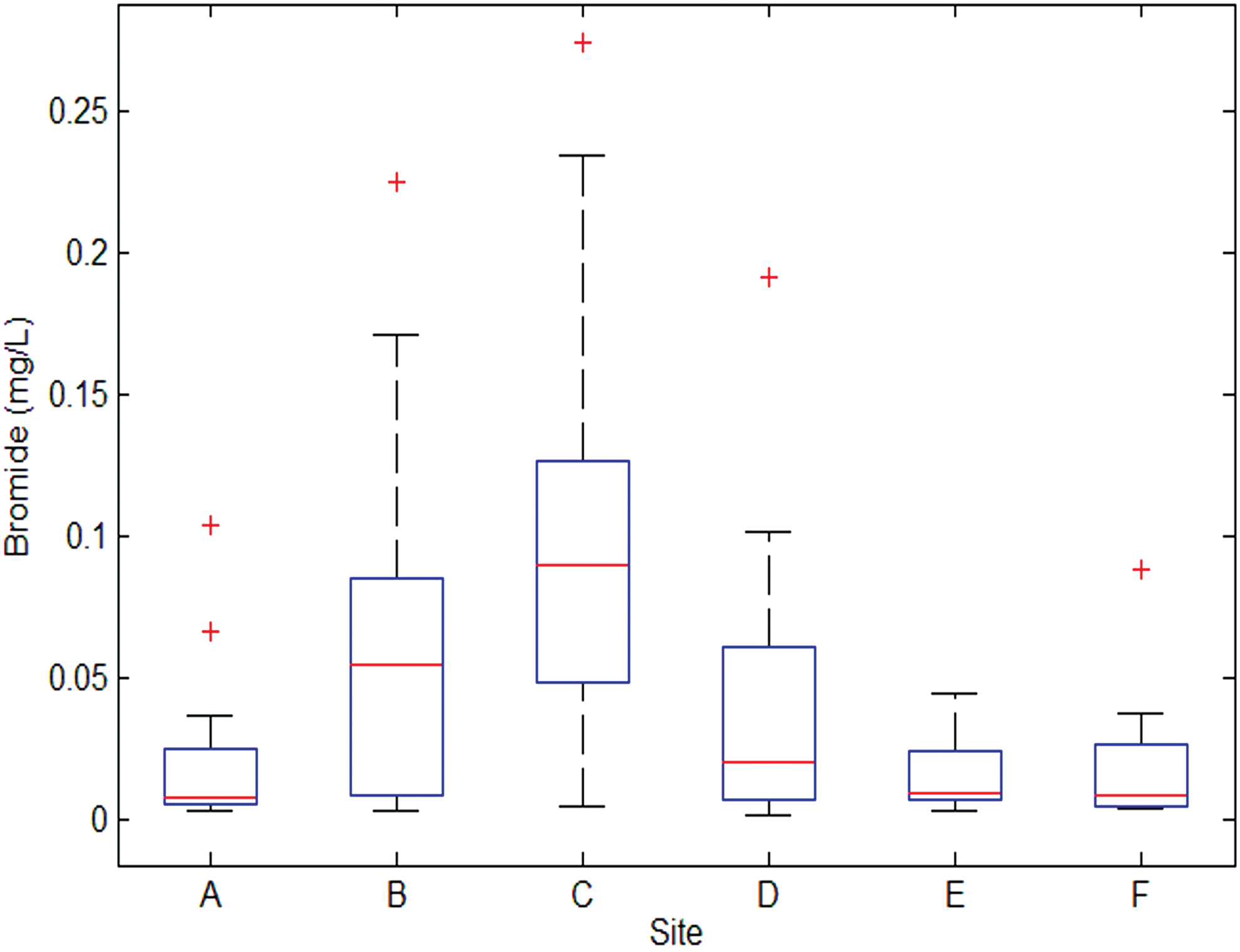
Boxplots of source water bromide concentration (mg/L) at each of the six sampling sites along the Monongahela River. Plots show median values, 75th and 25th quartiles (upper and lower ends of the box), most extreme nonoutlier values (ends of whiskers), and outliers (+ signs).

Variability in organic source water characteristics

Organic precursors were analyzed using commonly measured criteria, including DOC, UV₂₅₄, as well as through fluorescence EEMs, which were analyzed using PARAFAC analysis. Boxplots of DOC and UV₂₅₄ throughout the 3-year study at each of the six plants can be found in Supplementary Fig. S1 of the Supplementary Data. In general, DOC is very stable across the sites. UV₂₅₄ appears to be slightly more variable, but an ANOVA test indicates that mean UV₂₅₄ values are not significantly different across sites (p = 0.22). NOM is a well-known precursor for DBP formation, and UV₂₅₄ and DOC are often included in DBP prediction models (Edzwald et al., 1985; Reckhow et al., 1990; Kitis et al., 2002). However, these parameters are not correlated with TTHMs in this data set (R = 0.12 for DOC, 0.08 for UV₂₅₄). Although DOC and UV₂₅₄ provide some insight into organic carbon, their stability across multiple sites and seasons suggests these parameters are not providing enough information about variability to account for variability in observed TTHMs in finished water in the plants.

The EEM–PARAFAC analysis of the 109 sample EEMs yielded three components, C1, C2, and C3. Fluorescence maxima for the three components are shown in Table 2. All three components are found in the humic acid-like region, according to Chen et al. (2003). Furthermore, Sakai et al. (2015) found that EEMs with fluorescence signals in the “humic acid-like” region are highly correlated with TTHM formation. The three plots in Fig. 4 provide visual representations of the resultant PARAFAC components. Before considering the components as input modeling variables, their stability across sites was evaluated. Boxplots that illustrate the variability of the PARAFAC components and total fluorescence intensity, F_max, at each of the six sites throughout the 3-year study can be found in Supplementary Fig. S2 in the Supplementary Data.

FIG. 4.

EEMs of three components resulting from the EEM–PARAFAC analysis as follows: (a) C1, (b) C2, and (c) C3. EEM, excitation–emission matrices; PARAFAC, parallel factor analysis.

Table 2.

Fluorescence Maxima (Emission and Excitation) for Three PARAFAC Components—C1, C2, and C3

Component	Emission maxima (nm)	Excitation maxima (nm)
C1	440	346
C2	385	314
C3	495	394

PARAFAC, parallel factor analysis.

The four fluorescence characterizations—C1, C2, C3, and F_max—show some similar patterns at multiple sites. For example, Sites A and F and Sites D and E show similar central tendencies for each of the four fluorescence parameters. Overall, there is high variability in component values and F_max across the six sites, which is confirmed by ANOVA tests for each of the four fluorescence characterizations. ANOVA tests for C1, C2, C3, and F_max across the sites produced significant p values, 0.04, 0.003, 0.01, and 0.01, respectively. Although PARAFAC components show promise as DBP predictive parameters individually, they demonstrate poor linear fits with TTHMs (R² values of 0.10, 0.14, 0.07, and 0.11 for C1, C2, C3, and F_max, respectively). Previous work by Pifer and Fairey (2014) indicated high correlations between PARAFAC components and TTHM formation potential measured in the laboratory; however, direct prediction from a single component or F_max was not successful with these field samples.

Regression analysis

Source water constituents (i.e., NOM and bromide) are expected to influence DBP formation, and, thus, have the potential to predict concentrations of THM species. In this work, the utility of expanded NOM characterization along with bromide to predict THMs was examined. Operational characteristics were specifically excluded from modeling to ascertain whether models could be developed to account for source water variability throughout the region, independent of plant-specific operational characteristics.

Linear regressions were first developed for seven different response variables—TTHMs, chloroform (CHCl₃), bromodichloromethane (CHBrCl₂), dibromochloromethane (CHBr₂Cl), bromoform (CHBr₃), BIF, and percentage brominated THMs—using multiple input variables, including bromide, DOC, UV₂₅₄, and EEM–PARAFAC components. The untransformed and log-transformed variable regression models were statistically significant (F statistic p < 0.05), but showed poor to moderate R² values, ranging from 0.07 to 0.44 for untransformed variable regressions and 0.10 to 0.28 for the log-transformed variable regressions. Complete results and further discussion are presented in the Supplementary Data.

Classification trees

Classification trees were used to predict whether four key threshold values related to finished water DBPs—the TTHM MCL, 80% of the MCL, a BIF of 0.75, and 50% brominated THMs by mass—would be met. Two classification trees were created for each of the four binary response variables (based on the four threshold values)—one incorporating the three PARAFAC components (C1, C2, and C3) and one incorporating the ratios of each PARAFAC component to the total fluorescence intensity (C1/F_max, C2/F_max, and C3/F_max) as well as the total fluorescence intensity, F_max.

ROC curves for all eight classification trees are shown in Fig. 5. Figure 5a shows the ROC curves for the THM threshold trees (TTHM MCL and 80% of the TTHM MCL) and Fig. 5b shows the ROC curves for the brominated threshold trees (0.75 BIF and 50% Br THM). The plots in Fig. 5a show that incorporating component fractions provides stronger predictions than components for the two THM thresholds, and that when incorporating components, a better prediction is obtained for 80% of the TTHM MCL (64 μg/L) than for TTHM MCL. The plots in Fig. 5b show that incorporating components provides a stronger prediction than with component fractions for the two brominated thresholds, and that a better prediction is obtained for 0.75 BIF than for 50% Br THM. Overall, the 0.75 BIF component tree provides the strongest predictions of all eight trees, whereas the TTHM MCL component tree provides the weakest predictions.

FIG. 5.

Plot of ROC curves for classification trees. The TTHM MCL and 80% TTHM MCL (64 μg/L) trees are shown in (a) and the 0.75 BIF and 50% Br THM trees are shown in (b). The ROC curves for the component trees (C) are drawn in solid lines and the ROC curves for the component ratio (C/F) trees are drawn in dashed lines. Each response variable is designated by a different color, as shown in the legend. The dotted black line at Y = X shows a curve based on a random selection. AUC values are shown for the component trees in each plot. AUC, area under the curve; MCL, maximum contaminant level; ROC, receiver operator characteristic; THM, trihalomethane.

A summary of the performance of all eight classification trees—component and component ratio trees for predicting exceedance of each of the four threshold values—is shown in Table 3. The AUC values range from 0.73 to 0.92 and the accuracy values range from 0.76 to 0.83. Most of the trees have high and fairly similar sensitivity and specificity values (except for the component TTHM MCL tree and the component ratio 0.75 BIF tree), which means that the trees provide fairly balanced results.

Table 3.

Summary of Classification Tree Performance

	Components				Component ratios
Response Var.	AUC	Accuracy	Sensitivity	Specificity	AUC	Accuracy	Sensitivity	Specificity
TTHM MCL	0.730	0.83	0.25	0.96	0.867	0.83	0.80	0.84
80% MCL	0.811	0.77	0.66	0.81	0.875	0.83	0.72	0.88
0.75 BIF	0.924	0.83	0.61	0.96	0.894	0.80	0.53	0.94
50% Br THM	0.857	0.80	0.76	0.83	0.815	0.76	0.80	0.73

The table shows the AUC (area under the curve) value, accuracy, sensitivity, and specificity for the classification trees that use components (C1, C2, and C3) as fluorescence inputs and for the classification trees that use component ratios and total fluorescence (C1/F_max, C2/F_max, C3/F_max, and F_max) as fluorescence inputs for all four response variables—TTHM MCL, 80% of the TTHM MCL, BIF of 0.75, and 50% brominated THM.

AUC, area under the curve; ROC, receiver operator characteristic.

To evaluate the added value of fluorescence measurements, AUC values were determined for trees without fluorescence measurements. Based solely on DOC, UV₂₅₄, and bromide, AUC values are 0.60 for TTHM MCL, 0.56 for 80% TTHM MCL, 0.89 for 0.75 BIF, and 0.76 for 50% Br THM. All of these additional trees used the same minimum split as the eight classification trees incorporating the fluorescence measurements (25), except for the TTHM MCL tree that used a minimum split of 15 because a tree could not be created beyond a single node at a larger minimum split. The AUC values for trees without fluorescence measurements are overall worse than those for trees that incorporate fluorescence measurements, except for the 0.75 BIF, which gave similar results both with and without fluorescence measurements (AUC = 0.89 for the component ratio tree and AUC = 0.89 for the tree that omits fluorescence variables). These results indicate that, in general, fluorescence measurements improve classification tree predictions.

Predicting TTHM concentrations in excess of the MCL

The classification trees that predict exceedance of the TTHM MCL Regulation (TTHM concentration of 80 μg/L) are shown in Fig. 6. Figure 6a shows the tree that uses components as inputs (C1, C2, and C3) and Fig. 6b shows the tree that uses component ratios and total fluorescence (C1/F_max, C2/F_max, C3/F_max, and F_max) as inputs. Classification trees provide good fits of the data set, as demonstrated by the high-accuracy values and generally high-sensitivity and high-specificity values. Though the two trees performed similarly in accurately classifying instances, the component ratio tree (Fig. 6b) is more balanced in its classified outcomes, with nearly equal sensitivity and specificity values. The component tree (Fig. 6a) in contrast has a very high specificity (true negative rate) and very low sensitivity (true positive rate) because the tree slightly under-predicts exceeding the MCL, given in Table 3. The component classification tree classified very few instances as “exceed,” only 9 out of 109, although in reality 20 instances exceeded the MCL.

FIG. 6.

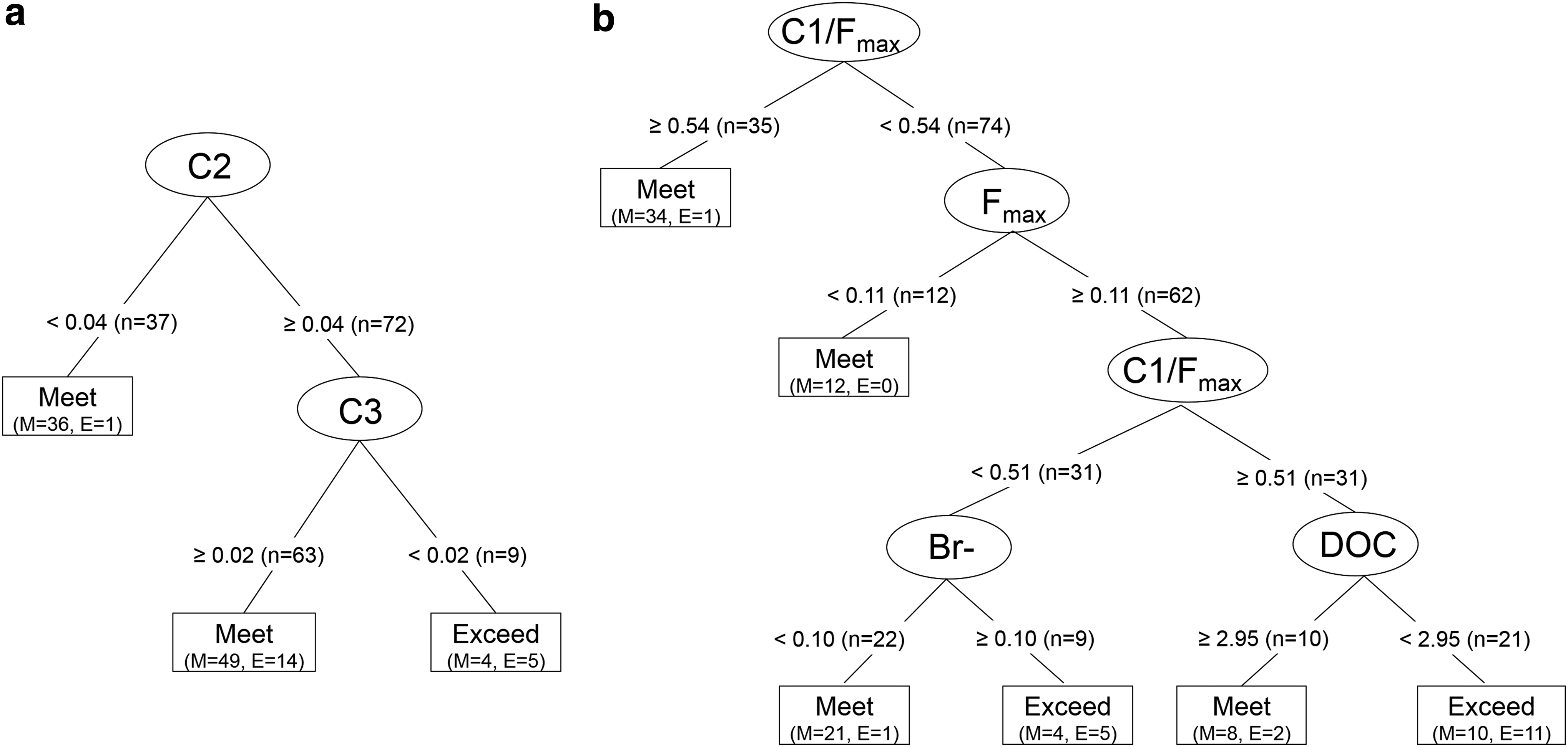
Classification trees created in R predict whether the TTHM MCL threshold is exceeded based on source water characteristics, including bromide, DOC, UV₂₅₄, and component subgroups: (a) the three PARAFAC components (C1, C2, and C3) and (b) the component ratios and total fluorescence intensity (C1/F_max, C2/F_max, C3/F_max, and F_max). The input parameters are drawn in ovals and the terminal nodes (indicating whether the TTHM MCL will be met or exceeded) are drawn in rectangles. Branches are labeled with the split of the input parameters and the number of instances (n) pertaining to the split. Terminal nodes are labeled with the overall outcome (“Meet” or “Exceed”) and the number of instances that actually meet (M) or exceed (E) the threshold. DOC, dissolved organic carbon; UV₂₅₄, ultraviolet absorbance at 254 nm.

The classification tree that uses components as inputs identifies C2 and C3 as the most important variables in predicting TTHM MCL exceedance, with C2 being the dominant input variable. According to the tree, instances with low C2 values (<0.04) are likely to meet the TTHM MCL. Outcomes for instances with high C2 values (≥0.04) depend on C3 values. Instances with high C2 values and high C3 values (≥0.02) are likely to meet the MCL, whereas instances with high C2 values and low C3 values (<0.02) are likely to exceed the MCL. The classification tree that uses component ratios and total fluorescence intensity as inputs identifies C1/F_max, F_max, bromide concentration, and DOC as the most important variables, with C1/F_max being the dominant input variable. According to the tree, when the C1/F_max ratio is high (≥0.54), instances are likely to meet the TTHM MCL. At lower C1/F_max values (<0.54), F_max is used to determine the outcome. Low C1/F_max and low F_max values (F_max < 0.11) generally meet the MCL. Instances are more likely to exceed the MCL when C1/F_max is low, F_max is high, and bromide concentration is high (≥0.10), or when Cl/F_max values are moderate (0.51–0.54), F_max is high, and DOC is low (<2.95).

A major difference between the two trees is the set of input variables included in each tree. The component classification tree incorporates only two fluorescence measurements (C2 and C3), whereas the component ratio classification tree incorporates two fluorescence measurements (C1/F_max and F_max), DOC, and bromide concentration. Despite these differences, both trees show a preference for fluorescence NOM measurements over DOC and UV₂₅₄, based on order of appearance in the tree and overall inclusion in the tree. Fluorescence measurements have also been found to be superior to SUVA in other studies when DOC is low (Lavonen et al., 2015). The inclusion of bromide in only one tree and at the bottom of the tree indicates that NOM characterization is more important than bromide concentration in predicting TTHM regulatory outcomes in this system, despite significant variability of bromide in the source water. The behavior of TTHM formation due to bromide concentration (increased likelihood of exceeding the MCL at higher bromide concentrations) is consistent with previous studies that found that increases in bromide concentration result in increased TTHMs (Hua et al., 2006; Navalon et al., 2008; Chowdhury et al., 2010).

Predicting TTHMs in excess of 80% of the MCL

Classification trees that predict exceedance of 80% of the TTHM MCL (64 μg/L) are shown in Fig. 7. Figure 7a illustrates the component classification tree (incorporating C1, C2, and C3) and Fig. 7b illustrates the component ratio tree (incorporating C1/F_max, C2/F_max, C3/F_max, and F_max). The 80% MCL (64 μg/L) classification trees look similar to the TTHM MCL trees, in which most of the same input variables were used. Both of the component trees incorporate C2 and C3 and the C2 split occurs at the same cut-off value; however, the 80% MCL tree also incorporates DOC. Both component ratio trees incorporate C1/F_max, F_max, and DOC, and the C1/F_max and first F_max splits occur at the same cut-off values; however, the TTHM MCL tree incorporates bromide, whereas the 80% MCL ratio tree incorporates C3/F_max. Of the four classification trees related to the regulatory TTHM MCL threshold (Figs. 6a, b and 7a, b), only one incorporates bromide, indicating that it is not as important as NOM characterization in determining whether or not the regulatory thresholds will be met. Although bromide has been found to increase DBP formation, many of the studies that report bromide being an important precursor in DBP formation incorporate synthetic laboratory samples that have higher concentrations of bromide than those found in these natural waters (Chang et al., 2001; Richardson et al., 2003; Hua et al., 2006; Navalon et al., 2008; Chowdhury et al., 2010; Hua and Reckhow, 2012; Watson et al., 2015). Additional discussion of the 80% TTHM MCL classification tree is found in the Supplementary Data.

FIG. 7.

Classification trees created in R predict whether the 80% of the TTHM MCL (64 μg/L) threshold is exceeded based on source water characteristics, including bromide, DOC, UV₂₅₄, and component subgroups: (a) the three PARAFAC components (C1, C2, and C3) and (b) the component ratios and total fluorescence intensity (C1/F_max, C2/F_max, C3/F_max, and F_max). The input parameters are drawn in ovals and the terminal nodes (indicating whether the TTHM MCL will be met or exceeded) are drawn in rectangles. Branches are labeled with the split of the input parameters and the number of instances (n) pertaining to the split. Terminal nodes are labeled with the overall outcome (“Meet” or “Exceed”) and the number of instances that actually meet (M) or exceed (E) the threshold.

Predicting BIF values in excess of 0.75

Classification trees that predict exceedance of the 0.75 BIF threshold are shown in Fig. 8. Figure 8a illustrates the component classification tree (incorporating C1, C2, and C3) and Fig. 8b illustrates the component ratio tree (incorporating C1/F_max, C2/F_max, C3/F_max, and F_max). The component classification tree (Fig. 8a) identifies bromide concentration, C1, and C2 as the most important variables, whereas the component ratio classification tree (Fig. 8b) identifies bromide and C3/F_max as the most important variables. In both classification trees, bromide is the first variable, meaning that it is the most indicative of the outcome behavior—exceeding or meeting the 0.75 BIF threshold. The inclusion of bromide as the dominant variable in both classification trees is consistent with previous research that found that bromide in the source water contributes to increased BIF in finished water (Rathburn, 1996a).

FIG. 8.

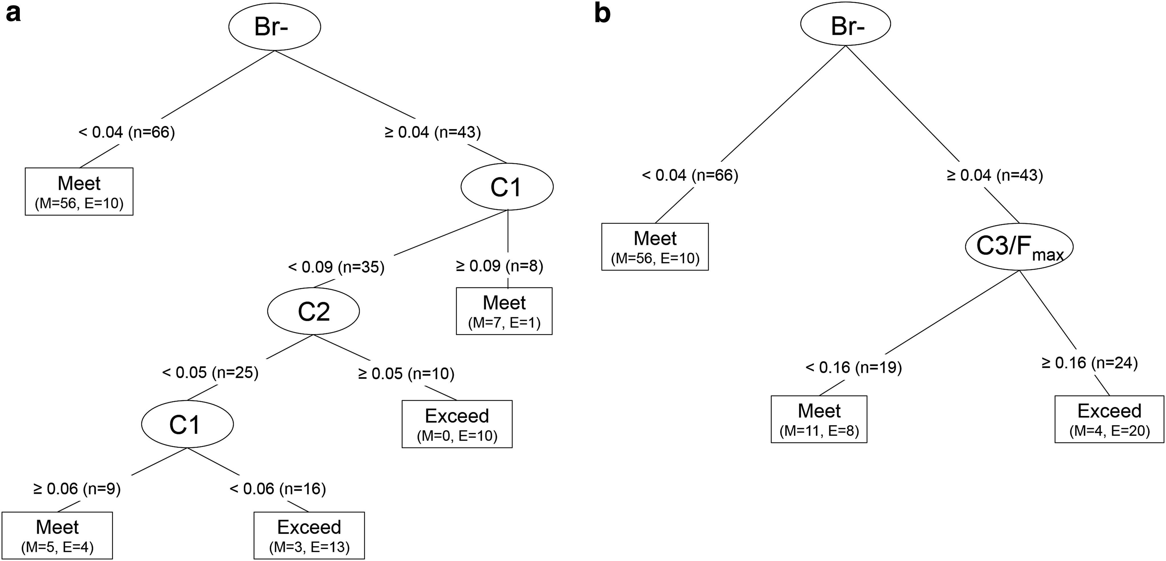
Classification trees created in R predict whether the 0.75 BIF (25% molar bromination) threshold is exceeded based on source water characteristics, including bromide, DOC, UV₂₅₄, and component subgroups: (a) the three PARAFAC components (C1, C2, and C3) and (b) the component ratios and total fluorescence intensity (C1/F_max, C2/F_max, C3/F_max, and F_max). The input parameters are drawn in ovals and the terminal nodes (indicating whether the TTHM MCL will be met or exceeded) are drawn in rectangles. Branches are labeled with the split of the input parameters and the number of instances (n) pertaining to the split. Terminal nodes are labeled with the overall outcome (“Meet” or “Exceed”) and the number of instances that actually meet (M) or exceed (E) the threshold.

Predicting THM bromination in excess of 50%

The classification trees that predict exceedance of 50% brominated THMs (by mass) are shown in Fig. 9. The component classification tree is illustrated in Fig. 9a and the component ratio classification tree is illustrated in Fig. 9b. The component classification tree identifies bromide, UV₂₅₄, C1, C2, and C3 as the most important input variables, and the component ratio classification tree identifies bromide, UV₂₅₄, and C1/F_max as the most important input variables for predicting whether the 50% brominated THMs by mass threshold will be exceeded. The results indicate that exceedance of the 50% brominated THMs threshold is dependent on both bromide and NOM characterization, with bromide being the most important. Furthermore, DOC is not included in either tree, indicating that the characterization of NOM is more important than the quantity in brominated THM formation (by mass), like the 0.75 BIF classification tree results. Both 50% Br THM classification trees show unexpected results—in three of the four, the exceedance scenarios contain lower bromide levels (<60 μg/L). It was expected that exceedances would more often occur in the high-bromide branches of the trees (≥60 μg/L) because higher bromide shifts DBPs toward brominated species (Chang et al., 2001; Richardson et al., 2003; Watson et al., 2015). However, the unexpected results may be due to a more complex relationship between bromide and NOM in DBP formation. Studies have shown that various water parameters, such as pH and temperature, as well as the character of the NOM affect the relative bromination of DBPs (Roccaro et al., 2013, 2014; Yan et al., 2016).

FIG. 9.

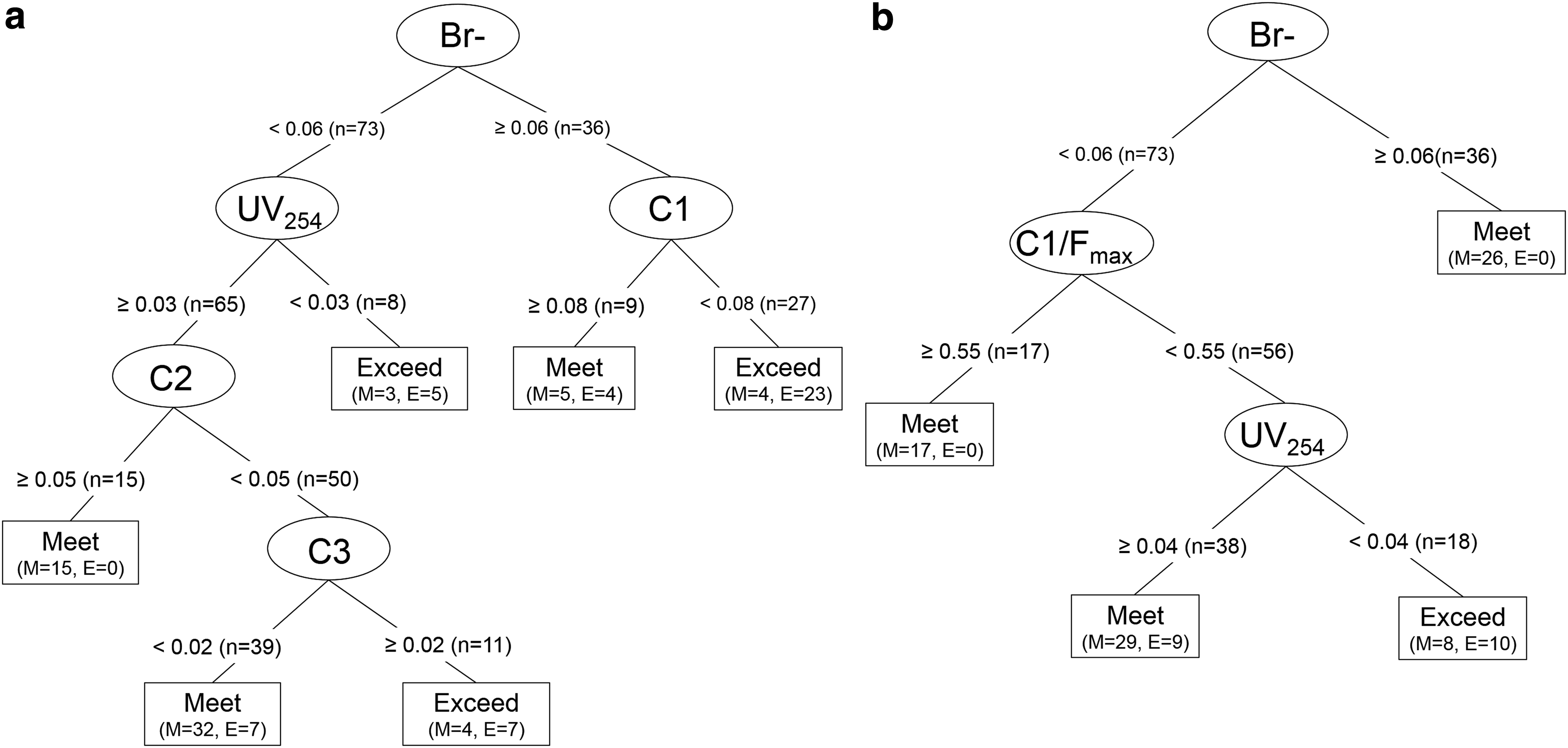
Classification trees created in R predict whether the 50% brominated THM (by mass) threshold is exceeded based on source water characteristics, including bromide, DOC, UV₂₅₄, and component subgroups: (a) the three PARAFAC components (C1, C2, and C3) and (b) the component ratios and total fluorescence intensity (C1/F_max, C2/F_max, C3/F_max, and F_max). The input parameters are drawn in ovals and the terminal nodes (indicating whether the TTHM MCL will be met or exceeded) are drawn in rectangles. Branches are labeled with the split of the input parameters and the number of instances (n) pertaining to the split. Terminal nodes are labeled with the overall outcome (“Meet” or “Exceed”) and the number of instances that actually meet (M) or exceed (E) the threshold.

The inclusion of fluorescence measurements in all eight classification trees, in addition to the higher AUC values for trees that include fluorescence measurements, demonstrates that fluorescence measurements are valuable parameters when classifying instances based on exceeding or meeting TTHM or Br THM thresholds. All four component trees (Figs. 6a, 7a, 8a, and 9a) include C2 and at least one other component (C1 or C3). In the TTHM component trees (Figs. 6a and 7a), C2 is the most important input variable. C2 has a similar peak to one of the two peaks in a PARAFAC component identified in another study (EM/EX = 381/219 [304]), which was found to be highly correlated with chloroform formation in a multivariate linear regression (Johnstone et al., 2009). In this study, chloroform is the dominant THM species. Three of the four component ratio trees (Figs. 6b, 7b, and 9b) include C1/F_max, and in all three of the trees, higher C1/F_max ratios (≥0.54) increase the likelihood of meeting the threshold. Finally, seven of the eight classification trees identify more than one NOM measurement as important input variables. The use of multiple NOM characterizations within the classification trees demonstrates the need for multiple NOM characterization techniques for effectively capturing the complexity and heterogeneity of NOM for predictive models.

Model validation across sites

To further evaluate the robustness of the classification trees across a spatially variable data set, additional classification trees were created on subsets of sites. The additional models, referred to as site validations (SVs), were performed by creating models based on five of the six sites (training data set) and then tested on the one remaining site (testing data set). Successful model generation from the SVs would suggest that a model created from multiple sites within a specific geographic region (such as the data set used in this study) could be applied to other sites within the region that were not originally incorporated into the model. Table 4 presents a summary of the accuracy values within the testing data set for the classification tree SV models that use the components (C1, C2, and C3) as inputs. Also contained in the summary are accuracy values for the models presented previously that were generated on the entire data set (referred to as “initial”). Overall, the SV models given in Table 4 show fairly high accuracy results. Except for 80% MCL SV 6 and 0.75 BIF SV 3 models, the accuracy values for the SV models are 0.50 or higher. Each of the four parameters has at least three SV models that correctly classify 65% or more of the test instances.

Table 4.

Summary of Accuracy Results for Site Validation Classification Trees Using Components (C1, C2, and C3)

Model	TTHM MCL	80% MCL	0.75 BIF	50% Brominated
Initial	0.83	0.77	0.83	0.80
SV 1	0.75	0.75	0.81	0.50
SV 2	0.82	0.74	0.82	0.65
SV 3	0.68	0.53	0.26	0.63
SV 4	0.60	0.50	0.75	0.70
SV 5	0.70	0.80	0.60	0.50
SV 6	0.50	0.20	0.70	0.80

Results are shown for the initial models (initial) and the six SV models for each of the four response parameters.

SV, site validation.

The same site cross-validations were performed for the classification tree models that used the component ratios and total fluorescence (C1/F_max, C2/F_max, and C3/F_max, F_max) as inputs. A summary of the results from these SV classification models is presented in Table 5. The SV models given in Table 5 also show fairly high accuracy results. With the exception of TTHM MCL SV 6, 0.75 BIF SV 3, 50% brominated SV 1, and 50% brominated SV 3, the accuracy results for the SV models are 0.50 or higher. Furthermore, each of the four parameters has at least two SV models that correctly classify 65% or more of the test instances. In general, the SV models show lower accuracy values than the initial models because they are developed and tested on a subset of the data.

Table 5.

Summary of Accuracy Results for Site Validation Classification Trees Using Component Ratios and Total Fluorescence (C1/F_max, C2/F_max, C3/F_max, and F_max)

Model	TTHM MCL	80% MCL	0.75 BIF	50% Brominated
Initial	0.83	0.83	0.80	0.76
SV 1	0.56	0.63	0.81	0.44
SV 2	0.88	0.74	0.76	0.65
SV 3	0.68	0.53	0.32	0.32
SV 4	0.65	0.60	0.70	0.65
SV 5	0.80	0.80	0.50	0.50
SV 6	0.40	0.50	0.80	0.80

Results are shown for the initial models (initial) and the six SV models for each of the four response parameters.

SV models demonstrate a reasonable level of accuracy; many of the SVs have accuracy values comparable to those of the initial models. Given that these models are fairly predictive across sites, there is potential for use of the models for other sites in the geographic region that were not originally included in the analysis. In addition, this suggests that the general method may provide insights into other geographic regions. Creating a classification model using data from multiple sites in a region may enable application at other drinking water facilities throughout that region.

Conclusions

Classification techniques demonstrate an improvement in predictive capability compared with regression models for predicting finished water quality based on source water characteristics alone for the data set used in this study, with 76–83% accuracy in correctly classifying instances. The classification trees are able to partition the input space of the explanatory variables to provide predictions that vary across this space. In addition, they are specifically structured and fit to provide optimal prediction of the threshold-defined categories for the dependent variables. Both sets of inputs—components (C1, C2, and C3) and component ratios (C1/F_max, C2/F_max, C3/F_max, and F_max)—demonstrated high sensitivity, specificity, and accuracy results within the classification trees. ROC curves indicated that the 0.75 BIF tree with component inputs was the best model overall.

NOM fluorescence measurements were chosen preferentially over UV₂₅₄ and DOC overall in the classification models, indicating their utility in DBP predictive models. C2 was identified as an important input variable in all four component classification trees and C1/F_max was identified as an important input variable in three of the four component ratio classification trees. In addition, the use of multiple NOM characterizations within many of the models indicates that multiple NOM characterizations that describe different features of the NOM are necessary for creating robust predictive models. Bromide was used in all Br THM models (0.75 BIF and 50% Br THM) but in only one of the TTHM models (TTHM MCL and 80% MCL), indicating that NOM may be more predictive of TTHM regulation than bromide in this region.

The success of the classification trees demonstrates an alternative method for assessing overall treatability of source water within a basin and for broadly predicting the finished water quality from source water characteristics. Classification techniques can be used to create regional source water models for other areas experiencing source water changes to assess potential challenges for compliance with operational and regulatory thresholds of interest.

Footnotes

Acknowledgments

The authors thank Dr. David Bergman, Dr. Clint Noack, Mr. Clint Mash, and Dr. Dana Peck for their assistance with the statistical analyses, including classification models, compositional data, and PARAFAC. Furthermore, the authors acknowledge funding support from the National Science Foundation through the NEEP-IGERT, the Colcom Foundation, and PITA (the Pennsylvania Infrastructure Technology Alliance). Additional support was provided to the corresponding author by a Dean's Fellowship from the Carnegie Institute of Technology, the Northrop Grumman Fellowship, and the Bradford and Diane Smith Graduate Fellowship, as well as an Achievement Rewards for College Scientists (ARCS) scholarship.

Author Disclosure Statement

No competing financial interests exist.

References

Abouleish

M.Y.

, and Wells

M.J.

(2015). Trihalomethane formation potential of aquatic and terrestrial fulvic and humic acids: Sorption on activated carbon. Sci. Total Environ., 521–522, 293.

Acero

J.L.

, Piriou

, and von Gunten

(2005). Kinetics and mechanisms of formation of bromophenols during drinking water chlorination: Assessment of taste and odor development. Water Res. 39, 2979.

Akaike

(1974). A new look at the statistical model identification. IEEE Trans. Automat. Contr., 19, 716.

Al-Omari

, Fayyad

, and Qader

(2004). Modeling trihalomethane formation for jabal amman water supply in Jordan. Environ. Model Assess., 9, 245.

Allard

, Tan

, Joll

C.A.

, and von Gunten

(2015). Mechanistic study on the formation of Cl-/Br-/I-trihalomethanes during chlorination/chloramination combined with a theoretical cytotoxicity evaluation. Environ. Sci. Technol., 49, 11105.

Amy

G.L.

, Chadik

P.A.

, and Chowdhury

Z.K.

(1987). Developing models for predicting trihalomethane formation potential and kinetics. J. Am. Water Works Assoc., 79, 89.

Ates

, Kitis

, and Yetis

(2007). Formation of chlorination by-products in waters with low SUVA—Correlations with SUVA and differential UV spectroscopy. Water Res. 41, 4139.

Awad

, van Leeuwen

, Chow

, Drikas

, Smernik

R.J.

, Chittleborough

D.J.

, and Bestland

(2016). Characterization of dissolved organic matter for prediction of trihalomethane formation potential in surface and sub-surface waters. J. Hazard. Mater., 308, 430.

Bae

, Kim

, and Kim

Y.J.

(2006). Decision algorithm based on data mining for coagulant type and dosage in water treatment systems. Wat. Sci. Tech., 53, 321.

10.

Baghoth

S.A.

, Sharma

S.K.

, and Amy

G.L.

(2011). Tracking natural organic matter (NOM) in a drinking water treatment plant using fluorescence excitation-emission matrices and PARAFAC. Water Res. 45, 797.

11.

Becker

, Stanford

, and Rosenfeldt

(2013). Guidance on complying with stage 2 D/DBP regulation. Water Res. Foundation. Web Report #4427.

12.

Bro

(1997). PARAFAC. Tutorial and applications. Chemometr. Intell. Lab., 38, 149.

13.

Cabaniss

S.E.

, and Shuman

M.S.

(1987). Synchronous fluorescence spectra of natural waters: Tracing sources of dissolved organic matter. Mar. Chem., 21, 37.

14.

Cantor

K.P.

, Villanueva

C.M.

, Silverman

D.T.

, Figueroa

J.D.

, Real

F.X.

, Garcia-Closas

, Malats

, Chanock

, Yeager

, Tardon

, Garcia-Closas

, Serra

, Carrato

, Castano-Vinyals

, Samanic

, Rothman

, and Kogevinas

(2010). Polymorphisms in GSTT1, GSTZ1, and CYP2E1, disinfection by-products, and risk of bladder cancer in Spain. Environ. Health Perspect., 118, 1545.

15.

Chambers

J.M.

, and Hastie

T.J.

(1992). Statistical Models in S. Pacific Grove, CA: Wadsworth and Brooks/Cole, p. 46.

16.

Chang

E.E.

, Lin

Y.P.

, and Chiang

P.C.

(2001). Effects of bromide on formation of THMs and HAAs. Chemosphere, 43, 1029.

17.

Chen

, and Westerhoff

(2010). Predicting disinfection by-product formation potential in water. Water Res. 44, 3755.

18.

Chen

, and Weisel

(1998). Halogenated DBP concentrations in a distribution system. J. Am. Water Works Assoc., 90, 151.

19.

Chen

, Westerhoff

, Leenheer

J.A.

, and Booksh

(2003). Fluorescence excitation-emission matrix regional integration to quantify spectra for dissolved organic matter. Environ. Sci. Technol., 37, 5701.

20.

Chowdhury

, Champagne

, and James McLellan

(2010). Investigating effects of bromide ions on trihalomethanes and developing model for predicting bromodichloromethane in drinking water. Water Res. 44, 2349.

21.

Chowdhury

, Champagne

, and McLellan

(2009). Models for predicting disinfection byproduct (DBP) formation in drinking waters: A chronological review. Sci. Total Environ., 407, 4189.

22.

Danileviciute

, Grazuleviciene

, Vencloviene

, Paulauskas

, and Nieuwenhuijsen

M.J.

(2012). Exposure to drinking water trihalomethanes and their association with low birth weight and small for gestational age in genetically susceptible women. Int. J. Environ. Res. Public Health, 9, 4470.

23.

Edzwald

J.K.

, Becker

W.C.

, and Wattier

K.L.

(1985). Surrogate parameters for monitoring organic matter and THM precursors. J. Am. Water Works Assoc., 77, 122.

24.

Elshorbagy

, Abu-Qdais

, and Elsheamy

(2000). Simulation of THM species in water distribution systems. Water Res. 34, 3431.

25.

EPA. (1995). Method 551.1: Determination of chlorination disinfection byproducts, chlorinated solvents, and halogenated pesticides/herbicides in drinking water by liquid-liquid extraction and gas chromatography with electron-capture detection. Revision 1.0.

26.

EPA. (2006). National primary drinking water regulations: Stage 2 disinfectants and disinfection byproducts rule. Fed. Reg., 71, 388.

27.

Francis

R.A.

, Small

M.J.

, and VanBriesen

J.M.

(2009). Multivariate distributions of disinfection by-products in chlorinated drinking water. Water Res. 43, 3453.

28.

Francis

R.A.

, VanBriesen

J.M.

, and Small

M.J.

(2010). Bayesian statistical modeling of disinfection byproduct (DBP) bromine incorporation in the ICR database. Environ. Sci. Technol., 44, 1232.

29.

Gallard

, Pellizzari

, Croué

J.P.

, and Legube

(2003). Rate constants of reactions of bromine with phenols in aqueous solution. Water Res. 37, 2883.

30.

Ged

E.C.

, Chadik

P.A.

, and Boyer

T.H.

(2015). Predictive capability of chlorination disinfection byproducts models. J. Environ. Manage., 149, 253.

31.

Gould

J.P.

, Fitchhorn

L.E.

, and Urheim

(1983). Formation of brominated trihalomethanes: Extent and kinetics. In Water Chlorination: Environmental Impact and Health Effects. Ann Arbor, MI: Ann Arbor Science Publishers, p. 297.

32.

Green

S.T.

, Small

M.J.

, and Casman

E.A.

(2009). Determinants of national diarrheal disease burden. Environ. Sci. Technol., 43, 993.

33.

Handke

(2008). Trihalomethane speciation and the relationship to elevated total dissolved solid concentrations affecting drinking water quality at systems utilizing the Monongahela River as a primary source during the 3rd and 4th quarters of 2008. Pennsylvania Department of Environmental Protection.

34.

Harrington

G.W.

, Chowdhury

Z.K.

, and Owen

D.M.

(1992). Developing a computer model to simulate DBP formation during water treatment. J. Am. Water Works Assoc., 84, 78.

35.

Harshman

R.A.

, and Lundy

M.E.

(1994). PARAFAC: Parallel factor analysis. Comput. Stat. Data An., 18, 39.

36.

Harvey

, Murphy

H.M.

, McBean

E.A.

, and Gharabaghi

(2015). Using data mining to understand drinking water advisories in small water systems: A case study of Ontario first nations drinking water supplies. Water Resour. Manag., 29, 5129.

37.

, Yan

, and Korshin

G.V.

(2015). Spectroscopic examination of effects of iodide on the chloramination of natural organic matter. Water Res. 70, 449.

38.

, and Hur

(2015). Conservative behavior of fluorescence EEM-PARAFAC components in resin fractionation processes and its applicability for characterizing dissolved organic matter. Water Res. 83, 217.

39.

Helsel

D.R.

(1990). Less than obvious—Statistical treatment of data below the detection limit. Environ. Sci. Technol., 24, 1766.

40.

Hua

, and Reckhow

D.A.

(2007a). Characterization of disinfection byproduct precursors based on hydrophobicity and molecular size. Environ. Sci. Technol., 41, 3309.

41.

Hua

, and Reckhow

D.A.

(2007b). Comparison of disinfection byproduct formation from chlorine and alternative disinfectants. Water Res. 41, 1667.

42.

Hua

, and Reckhow

D.A.

(2012). Evaluation of bromine substitution factors of DBPs during chlorination and chloramination. Water Res. 46, 4208.

43.

Hua

, Reckhow

D.A.

, and Abusallout

(2015). Correlation between SUVA and DBP formation during chlorination and chloramination of NOM fractions from different sources. Chemosphere, 130, 82.

44.

Hua

, Reckhow

D.A.

, and Kim

(2006). Effect of bromide and iodide ions on the formation and speciation of disinfection byproducts during chlorination. Environ. Sci. Technol., 40, 3050.

45.

Johnstone

D.W.

, Sanchez

N.P.

, and Miller

C.M.

(2009). Parallel factor analysis of excitation–emission matrices to assess drinking water disinfection byproduct formation during a peak formation period. Environ. Eng. Sci., 26, 1551.

46.

Kawamoto

, and Makihata

(2004). Distribution of bromine/chlorine-containing disinfection by-products in tap water from different water sources in the hyogo prefecture. J. Health Sci., 50, 235.

47.

King

W.D.

, and Marrett

L.D.

(1996). Case-control study of bladder cancer and chlorination by-products in treated water (Ontario, Canada). Cancer Cause Control. 7, 596.

48.

Kitis

, Karanfil

, Kilduff

J.E.

, and Wigton

(2001). The reactivity of natural organic matter to disinfection by-products formation and its relation to specific ultraviolet absorbance. Wat. Sci. Tech., 43, 9.

49.

Kitis

, Karanfil

, Wigton

, and Kilduff

J.E.

(2002). Probing reactivity of dissolved organic matter for disinfection by-product formation using XAD-8 resin adsorption and ultrafiltration fractionation. Water Res. 36, 3834.

50.

Korn

, Andrews

R.C.

, and Escobar

M.D.

(2002). Development of chlorine dioxide-related by-product models for drinking water treatment. Water Res. 36, 330.

51.

Kulkarni

, and Chellam

(2010). Disinfection by-product formation following chlorination of drinking water: Artificial neural network models and changes in speciation with treatment. Sci. Total Environ., 408, 4202.

52.

Kumar

, Forand

, Babcock

, Richter

, Hart

, and Hwang

S.A.

(2014). Total trihalomethanes in public drinking water supply and birth outcomes: A cross-sectional study. Matern Child Health J. 18, 996.

53.

Lavonen

E.E.

, Kothawala

D.N.

, Tranvik

L.J.

, Gonsior

, Schmitt-Kopplin

, and Kohler

S.J.

(2015). Tracking changes in the optical properties and molecular composition of dissolved organic matter during drinking water production. Water Res. 85, 286.

54.

Lawaetz

A.J.

, and Stedmon

C.A.

(2009). Fluorescence intensity calibration using the Raman scatter peak of water. Appl. Spectrosc., 63, 936.

55.

, Zhao

, Mao

, Liu

, and Qu

(2014a). Characterization of dissolved organic matter from surface waters with low to high dissolved organic carbon and the related disinfection byproduct formation potential. J. Hazard. Mater., 271, 228.

56.

, Clark

R.M.

, Buchberger

S.G.

, and Jeffrey Yang

(2014b). Evaluation of climate change impact on drinking water treatment plant operation. J. Environ. Eng., 140, A4014005.

57.

Liang

, and Singer

(2003). Factors influencing the formation and relative distribution of haloacetic acids and trihalomethanes in drinking water. Environ. Sci. Technol., 37, 2920.

58.

, Zhang

, Ma

, and Chen

(2009). Evaluation of disinfection by-products formation during chlorination and chloramination of dissolved natural organic matter fractions isolated from a filtered river water. J. Hazard. Mater., 162, 140.

59.

Mao

, Wang

, Yang

, Wang

, and Xie

Y.F.

(2014). Effects of ozonation on disinfection byproduct formation and speciation during subsequent chlorination. Chemosphere. 117, 515.

60.

Mayer

B.K.

, Daugherty

, and Abbaszadegan

(2015). Evaluation of the relationship between bulk organic precursors and disinfection byproduct formation for advanced oxidation processes. Chemosphere. 121, 39.

61.

Montesinos

, and Gallego

(2013). Speciation of common volatile halogenated disinfection by-products in tap water under different oxidising agents. J. Chromatogr., 1310, 113.

62.

Murphy

H.M.

, Bhatti

M.A.

, Harvey

, and McBean

E.A.

(2016). Using decision trees to predict drinking water advisories in small water systems. J. Am. Water Works Assoc. 108.

63.

Murphy

K.R.

, Stedmon

C.A.

, Graeber

, and Bro

(2013). Fluorescence spectroscopy and multi-way techniques. PARAFAC. Anal. Methods. 5, 6557.

64.

Najm

I.N.

, Patania

N.L.

, Jacangelo

J.G.

, and Krasner

S.W.

(1994). Evaluating surrogates for disinfection by-products. J. Am. Water Works Assoc., 86, 98.

65.

Navalon

, Alvaro

, and Garcia

(2008). Carbohydrates as trihalomethanes precursors. Influence of pH and the presence of Cl(-) and Br(-) on trihalomethane formation potential. Water Res., 42, 3990.

66.

Nokes

, Fenton

, and Randall

(1999). Modeling the formation of brominated trihalomethanes in chlorinated drinking waters. Water Res. 33, 3557.

67.

Obolensky

, and Singer

P.C.

(2005). Halogen substitution patterns among disinfection byproducts in the information collection rule database. Environ. Sci. Technol., 39, 2719.

68.

Obolensky

, and Singer

P.C.

(2008). Development and interpretation of disinfection byproduct formation models using the information collection rule database. Environ. Sci. Technol., 42, 5654.

69.

Pifer

A.D.

, and Fairey

J.L.

(2012). Improving on SUVA 254 using fluorescence-PARAFAC analysis and asymmetric flow-field flow fractionation for assessing disinfection byproduct formation and control. Water Res. 46, 2927.

70.

Pifer

A.D.

, and Fairey

J.L.

(2014). Suitability of organic matter surrogates to predict trihalomethane formation in drinking water sources. Environ. Eng. Sci., 31, 117.

71.

Pifer

A.D.

, Miskin

D.R.

, Cousins

S.L.

, and Fairey

J.L.

(2011). Coupling asymmetric flow-field flow fractionation and fluorescence parallel factor analysis reveals stratification of dissolved organic matter in a drinking water reservoir. J. Chromatogr., 1218, 4167.

72.

Pisarenko

A.N.

, Stanford

B.D.

, Snyder

S.A.

, Rivera

S.B.

, and Boal

A.K.

(2013). Investigation of the use of chlorine based advanced oxidation in surface water: Oxidation of natural organic matter and formation of disinfection byproducts. J. Adv. Oxid. Technol., 16, 137.

73.

Plewa

M.J.

, Kargalioglu

, Vankerk

, Minear

R.A.

, and Wagner

E.D.

(2002). Mammalian cell cytotoxicity and genotoxicity analysis of drinking water disinfection by-products. Environ. Mol. Mutagen., 40, 134.

74.

Rathburn

R.E.

(1996a). Bromine incorporation factors for triahlomethane formation for the Mississippi, Missouri, and Ohio Rivers. Sci. Total Environ., 192, 111.

75.

Rathburn

R.E.

(1996b). Speciation of trihalomethane mixtures for the Mississippi, Missouri, and Ohio Rivers. Sci. Total Environ., 180, 125.

76.

RCoreTeam. (2015). R: A Language and Environment for Statistical Computing. Vienna, Austria: R Foundation for Statistical Computing. Available at: www.R-project.org/ accessed November 9, 2015.

77.

Reckhow

D.A.

, Singer

P.C.

, and Malcolm

R.L.

(1990). Chlorination of humic materials: Byproduct formation and chemical interpretations. Environ. Sci. Technol., 24, 1655.

78.

Regli

, Chen

, Messner

, Elovitz

M.S.

, Letkiewicz

, Pegram

, Pepping

T.J.

, Richardson

, and Wright

J.M.

(2015). Estimating potential increased bladder cancer risk due to increased bromide concentrations in sources of disinfected drinking waters. Environ. Sci. Technol., 49, 13094.

79.

Richardson

S.D.

, Plewa

M.J.

, Wagner

E.D.

, Schoeny

, and Demarini

D.M.

(2007). Occurrence, genotoxicity, and carcinogenicity of regulated and emerging disinfection by-products in drinking water: A review and roadmap for research. Mutat. Res., 636, 178.

80.

Richardson

S.D.

, Thruston

, Alfred

, Rav-Acha

, Groisman

, Popilevsky

, Juraev

, Glezer

, McKague

A.B.

, Plewa

M.J.

, and Wagner

E.D.

(2003). Tribromopyrrole, brominated acids, and other disinfection byproducts produced by disinfection of drinking water rich in bromide. Environ. Sci. Technol., 37, 3782.

81.

Roberson

J.A.

, Cromwell

J.E.

III , Krasner

S.W.

, and McGuire

M.J.

(1995). The D/DBP Rule: Where did the numbers come from?. J. Am. Water Works Assoc., 87, 46.

82.

Roccaro

, Chang

H.S.

, Vagliasindi

F.G.

, and Korshin

G.V.

(2008). Differential absorbance study of effects of temperature on chlorine consumption and formation of disinfection by-products in chlorinated water. Water Res. 42, 1879.

83.

Roccaro

, Chang

H.S.

, Vagliasindi

F.G.

, and Korshin

G.V.

(2013). Modeling bromide effects on yields and speciation of dihaloacetonitriles formed in chlorinated drinking water. Water Res. 47, 5995.

84.

Roccaro

, Korshin

G.V.

, Cook

, Chow

C.W.

, and Drikas

(2014). Effects of pH on the speciation coefficients in models of bromide influence on the formation of trihalomethanes and haloacetic acids. Water Res. 62, 117.

85.

Roccaro

, and Vagliasindi

F.G.A.

(2010). Monitoring emerging chlorination by-products in drinking water using UV-absorbance and fluorescence indexes. Desalin. Water Treat., 23, 118.

86.

Roccaro

, Vagliasindi

F.G.A.

, and Korshin

G.V.

(2009). Changes in NOM fluorescence caused by chlorination and their associations with disinfection by-products formation. Environ. Sci. Technol., 43, 724.

87.

Rodriguez

, Serodes

, Levallois

, and Proulx

(2007). Chlorinated disinfection by-products in drinking water according to source, treatment, season, and distribution location. J. Environ. Eng. Sci., 6, 355.

88.

Rodriguez

M.J.

, Serodes

J.B.

, and Levallois

(2004). Behavior of trihalomethanes and haloacetic acids in a drinking water distribution system. Water Res. 38, 4367.

89.

Sadiq

, and Rodriguez

M.J.

(2004). Disinfection by-products (DBPs) in drinking water and predictive models for their occurrence: A review. Sci. Total Environ., 321, 21.

90.

Sakai

, Tokuhara

, Murakami

, Kosaka

, Oguma

, and Takizawa

(2015). Comparison of chlorination and chloramination in carbonaceous and nitrogenous disinfection byproduct formation potentials with prolonged contact time. Water Res. 88, 661.

91.

Sanchez

N.P.

, Skeriotis

A.T.

, and Miller

C.M.

(2013). Assessment of dissolved organic matter fluorescence PARAFAC components before and after coagulation-filtration in a full scale water treatment plant. Water Res. 47, 1679.

92.

Sanchez

N.P.

, Skeriotis

A.T.

, and Miller

C.M.

(2014). A PARAFAC-based long-term assessment of DOM in a multi-coagulant drinking water treatment scheme. Environ. Sci. Technol., 48, 1582.

93.

Shutova

, Baker

, Bridgeman

, and Henderson

R.K.

(2014). Spectroscopic characterisation of dissolved organic matter changes in drinking water treatment: From PARAFAC analysis to online monitoring wavelengths. Water Res. 54, 159.

94.

Sierra

M.M.D.S.

, Donard

O.F.X.

, Lamotte

, Belin

, and Ewald

(1994). Fluorescence spectroscopy of coastal and marine waters. Mar. Chem., 47, 127.

95.

Sing

, Sander

, Beerenwinkel

, and Lengauer

(2005). ROCR: Visualizing classifier performance in R. Bioinformatics. 21, 3940.

96.

Singer

P.C.

, and Chang

S.D.

(1989). Correlations between trihalomethanes and total organic halides formed during water treatment. J. Am. Water Works Assoc., 81, 61.

97.

Singer

, Weinberg

, Brophy

, Liang

, Roberts

, Grisstede

, Krasner

, Baribeau

, Arora

, and Najm

(2002). Relative Dominance of Haloacetic Acids and Trihalomethanes in Treated Drinking Water. Denver, CO: American Water Works Association Research Foundation.

98.

Sohn

, Amy

, Cho

, Lee

, and Yoon

(2004). Disinfectant decay and disinfection by-products formation model development: Chlorination and ozonation by-products. Water Res. 38, 2461.

99.

Sohn

, Amy

, and Yoon

(2006). Bromide ion incorporation into brominated disinfection by-products. Water Air Soil Poll. 174, 265.

100.

States

, Cyprych

, Stoner

, Wydra

, Kuchta

, Monnell

, and Casson

(2013). Brominated THMs in drinking water: A possible link to marcellus shale and other wastewaters. J. Am. Water Works Assoc., 105, E432.

101.

Stedmon

C.A.

, and Bro

(2008). Characterizing dissolved organic matter fluorescence with parallel factor analysis: A tutorial. Limnol. Oceanogr.: Methods., 6, 572.

102.

Stedmon

C.A.

, and Markager

(2005). Resolving the variability in dissolved organic matter fluorescence in a temperate estuary and its catchment using PARAFAC analysis. Limnol. Oceanogr., 50, 686.

103.

Stedmon

C.A.

, Markager

, and Bro

(2003). Tracing dissolved organic matter in aquatic environments using a new approach to fluorescence spectroscopy. Mar. Chem., 82, 239.

104.

Tian

, Liu

, Guo

, Liu

, Luo

, and Qu

(2013). Chlorination and chloramination of high-bromide natural water: DBPs species transformation. Sep. Purif. Technol., 102, 86.

105.

Trueman

B.F.

, MacIsaac

S.A.

, Stoddart

A.K.

, and Gagnon

G.A.

(2016). Prediction of disinfection by-product formation in drinking water via fluorescence spectroscopy. Environ. Sci.: Water Res. Technol., 2, 383.

106.

Villanueva

C.M.

, Cantor

K.P.

, Cordier

, Jaakkola

J.J. K.

, King

W.D.

, Lynch

C.F.

, Porru

, and Kogevinas

(2004). Disinfection byproducts and bladder cancer. Epidemiology, 15, 357.

107.

Wang

, Wilson

J.M.

, and VanBriesen

J.M.

(2015). The effect of sampling strategies on assessment of water quality criteria attainment. J. Environ. Manage., 154, 33.

108.

Watson

, Farre

M.J.

, Birt

, McGree

, and Knight

(2015). Predictive models for water sources with high susceptibility for bromine-containing disinfection by-product formation: Implications for water treatment. Environ. Sci. Pollut. Res. Int., 22, 1963.

109.

Weaver

J.W.

, Xu

, and Mravik

S.C.

(2015). Scenario analysis of the impact on drinking water intakes from bromide in the discharge of treated oil and gas wastewater. J. Environ. Eng. DOI: 10.1061/(ASCE)EE.1943–7870.0000968.

110.

Weishaar

J.L.

, Aiken

G.R.

, Bergamaschi

B.A.

, Fram

M.S.

, Fujii

, and Mopper

(2003). Evaluation of specific ultraviolet absorbance as an indicator of the chemical composition and reactivity of dissolved organic carbon. Environ. Sci. Technol., 37, 4702.

111.

Westerhoff

, Debroux

, Amy

G.L.

, Gatel

, Mary

, and Cavard

(2000). Applying DBP models to full-scale plants. Am. Water Works Assoc., 92, 89.

112.

Wilson

J.M.

(2013). Challenges for drinking water plants from energy extraction activities. PhD Dissertation. Dept. of Civil & Environmental Engineering, Carnegie Mellon University, Pittsburgh, PA.

113.

Wilson

J.M.

, and Van Briesen

J.M.

(2013). Source water changes and energy extraction activities in the Monongahela River. 2009–2012. Environ. Sci. Technol., 47, 12575.

114.

Yan

, Li

, Roccaro

, and Korshin

G.V.

(2016). Ternary model of the speciation of I-/Br-/Cl-trihalomethanes formed in chloraminated surface waters. Environ. Sci. Technol., 50, 4468.

115.

Yang

, Hur

, Lee

, Chang

S.W.

, and Shin

H.S.

(2015a). Dynamics of dissolved organic matter during four storm events in two forest streams: Source, export, and implications for harmful disinfection byproduct formation. Environ. Sci. Pollut. Res. Int., 22, 9173.

116.

Yang

, Kim

, Uzun

, Karanfil

, and Hur

(2015b). Assessing trihalomethanes (THMs) and N-nitrosodimethylamine (NDMA) formation potentials in drinking water treatment plants using fluorescence spectroscopy and parallel factor analysis. Chemosphere. 121, 84.

Supplementary Material

Please find the following supplemental material available below.

For Open Access articles published under a Creative Commons License, all supplemental material carries the same license as the article it is associated with.

For non-Open Access articles published, all supplemental material carries a non-exclusive license, and permission requests for re-use of supplemental material or any part of supplemental material shall be sent directly to the copyright owner as specified in the copyright notice associated with the article.

0.00 MB

0.34 MB