Low-Cost Stand-Alone System for Real-Time Hydrological Monitoring

Abstract

Water resource managers and scientists have recognized the need for data at spatial and temporal resolutions relevant to the hydrological cycle. The dearth of hydrological data sets has been noted as a critical barrier to developing effective water resource management strategies. Limited funding has been noted as a major contributing factor to the limited establishment of sustainable environmental monitoring networks to capture these data sets. To address these concerns, an inexpensive real-time hydrological monitoring station (RTHS) was designed to collect data with similar performance to existing commercially available sensors. The RTHS was built with both commercially available and custom-engineered components, using enabling technology to reduce capital and operations and maintenance costs. The RTHS incorporated a modular design for easy integration of multiple sensors and implementation of upgrades with less expensive and more reliable components as emerging technologies become available. Inexpensive stage height, water temperature, and all-season precipitation sensors were designed, fabricated, and tested in house. Integration of components into a comprehensive hydrological monitoring system required custom hardware designs and software routines. Controlled laboratory and field evaluations with a colocated research-grade sensor indicated that the designed precipitation gauge provides a low-cost alternative with comparable performance to commercially available off-the-shelf sensors. The designed stage height sensor performed well in laboratory evaluations and interobservatory comparisons at independently operated stations in the Hudson River watershed as demonstrated by strong correlations (R² = 0.99, root mean square discrepancy = 1.4–3.2 cm) between stage height data sets.

Introduction

Dramatic consequences of hydrological variability including changes in precipitation, drought, and extreme flood have determined broad features of human settlement and commerce since ancient times (Maidment, 1993). It has been predicted that hydrological events in many areas will potentially become more variable and severe (Barnett et al., 2005; Huntington, 2006) and difficult to predict in the foreseeable future (Jackson et al., 2001; Revenga et al., 2005; Parry et al., 2007). Accurate representation of spatial and temporal variability of climate-forcing data, especially precipitation, has proven to be a challenge for hydrological modeling due to limited availability of these data sets. Failure to incorporate such variability has been attributed to the introduction of significant uncertainty to hydrological modeling efforts (Jordan, 2000; Andreassian et al., 2001; Schuurmans and Bierkens, 2007; Villarni et al., 2008) that limits capability of these models to provide reliable hydrological predictions. Montgomery et al. (2007) emphasized the need for an integrated environmental observatory network to capture this variability for improved forecasting and management of critical water resources. Recent research pointed to a dearth of water resource data as a critical barrier to implementing improved management practices (Gilbert, 2010). Despite the need for and value of high-frequency data in hydrological modeling applications, the U.S. Geological Survey (USGS) stage height gauge stations have gone through a persistent and decades-long reduction (Mui et al., 2010).

Limited funding represents a major challenge to providing hydrological data at relevant spatial and temporal resolutions for water resource management decision applications (Harmancioglu and Alpaslan, 1992). Wang et al. (2008) note the high costs associated with operation and maintenance (O&M) and development of the sensor systems and supporting infrastructures as reasons for the lack of dense precipitation gauge networks. Absence of an integrated systems approach to hydrological monitoring can further increase costs. For example, the National Weather Service (NWS) and USGS operate and maintain independent observation networks to measure meteorological (e.g., precipitation and wind speed/direction) and stream flow/stage height data sets, respectively. Where and when possible, alleviation of redundancies associated with the operation of similar but separate observatories (e.g., stage height and meteorology stations) may result in unit data costs reductions.

We have applied a comprehensive, iterative, adaptive (CIA) process to develop an integrated inexpensive hydrological monitoring system. In the CIA process, design criteria were redefined as a function of system and/or component strengths and deficiencies identified during evaluations at increasing levels of operation (e.g., prototype, laboratory, and limited-field and full-field scales). The refined design criteria were then incorporated in subsequent design revisions that took advantage of evolving and perhaps more cost-effective technologies (e.g., single-board computers, microcontroller, and low-cost integrated circuits). Upgrades borne through this process are then routinely implemented into the complete network at rates defined by standard service intervals.

Through application of the CIA process, the real-time hydrological monitoring station (RTHS) was developed to meet the following design criteria: low power consumption, low capital costs, robust, real-time autonomous four-season operation, low maintenance, and modularity. The final design included a combination of commercially available sensors (i.e., air temperature, relative humidity, wind speed/direction, and barometric pressure) and low-cost in-house designed sensors (i.e., precipitation, stage height, and water temperature). System modularity has permitted expansion of measured parameters (e.g., water quality) and integration of system upgrades in subsequent development iterations. Flexibility of the RTHS designs has enabled both grid-tied installation and the preferred independent solar-powered installation. Station mounting configurations varied by site-specific characteristics including access to communication and power. Open source software was applied to automatically upload the measured data sets into the standardized Consortium of Universities for the Advancement of Hydrologic Science, Inc. (CUAHSI) hydrological information system (HIS) for broad dissemination (Piasecki et al., 2010).

This article describes in detail the design of our developed all-season precipitation gauge and stage height sensors. Sensor performance evaluations include a combination of laboratory test results and comparisons against commercially available sensors. Results from these evaluations demonstrate the reliability and ruggedness of the RTHS.

Materials and Methods

The RTHS design includes three major subsystems including (1) in situ sensors, (2) computing infrastructure, and (3) data management and communication (Fig. 1). Descriptions of each subsystem are provided hereunder.

FIG. 1.

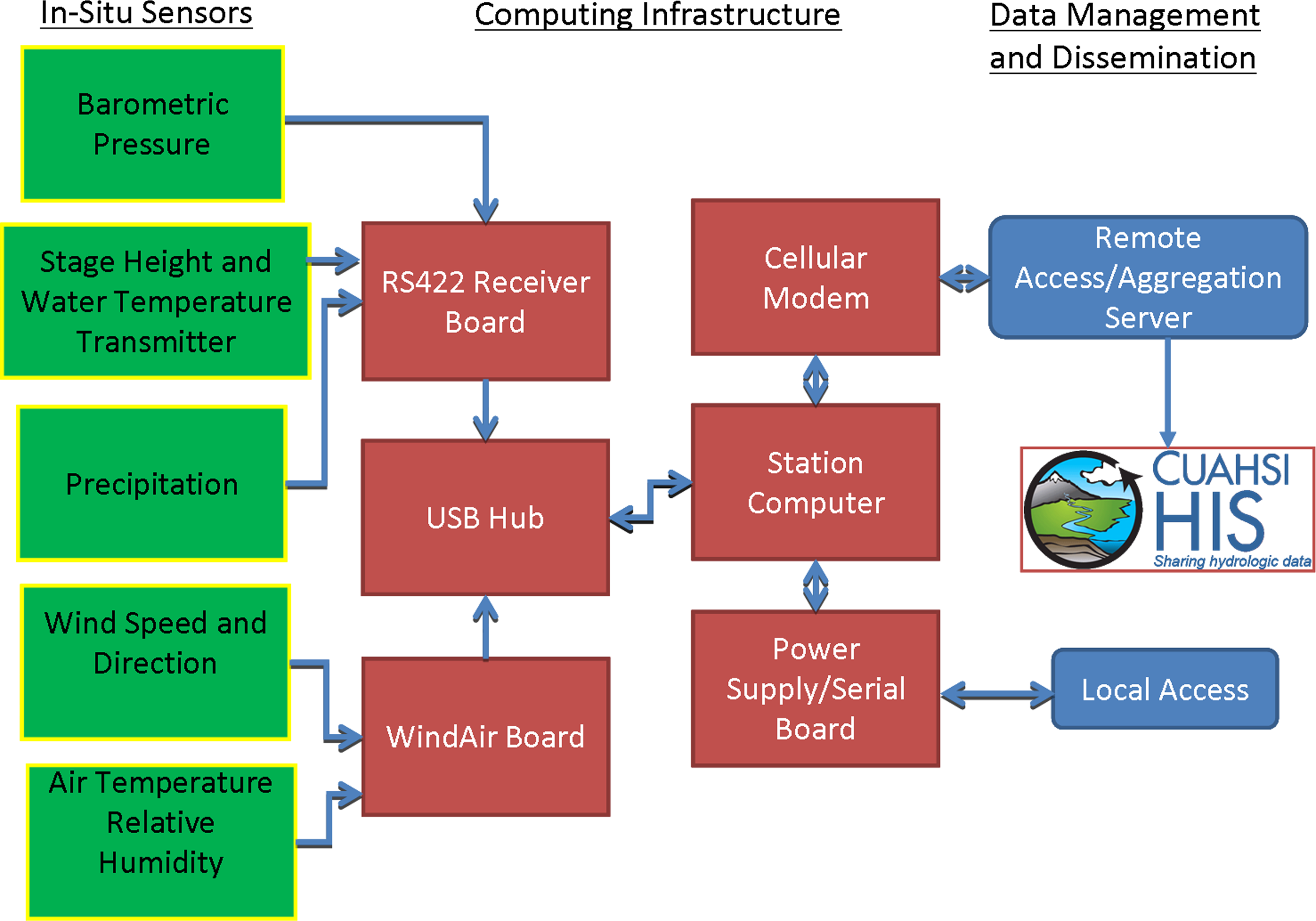
RTHS system overview. RTHS, real-time hydrological monitoring station.

In situ sensors

A combination of commercial off-the-shelf (COTS) (Table 1) and in-house designed sensors was selected for use in the RTHS based on cost and sensor performance criteria. All COTS sensors, except barometric pressure, were coupled to an in-house designed printed circuit board, “WindAir.” In-house designed sensors included (1) stage height sensor and (2) all-season precipitation gauge. Both COTS and in-house designed sensors were integrated into the RTHS system through enabling technologies (e.g., microcontroller and single-board computer) for real-time measurement and dissemination of the mentioned hydrological parameters.

Table 1.

RTHS COTS Atmospheric Sensor Specifications and Performance Ratings

Parameter	Manufacturer	Model	Range (sensitivity)	Accuracy
Air temperature	Vaisala	HMP60	−40°C to 60°C	0.6°C
Relative humidity	Vaisala	HMP60	0% to 100%	3–5%
Wind speed	Novalynx	200-WS-05F	0–99 MPH	1 MPH or ±3%
Wind direction	Novalynx	200-WS-05F	0–360°	±3%
Barometric pressure	Bosch	BMP085	300–1100 hPa	±1.5 hPa

COTS, commercial off-the-shelf; RTHS, real-time hydrological monitoring station.

Precipitation gauge

Selection of a weighing-type precipitation gauge in the RTHS sensor suite is based on its relatively low power consumption and applicability in subfreezing conditions that typify our study area that spans latitudes 40°N–45°N. Descriptions of other gauges evaluated including float and siphon and the tipping-bucket types can be found in Raghunath (2006). Traditional heated tipping bucket gauges have significant power requirements, as much as 320 watts continuously in winter months that effectively make remote installations impractical. The float type is not suitable for measuring snow in subfreezing conditions. Our weighing-type precipitation gauge is based on recently developed integrated circuit technology and reliable pressure transducers that draw less than 1 watt at 12 volts. The precipitation gauge design includes an aluminum collection chamber (19.7 cm inside diameter), low-range pressure sensor, high-range pressure sensor, amplifier circuit, 16-bit analog to digital converter (ADC), and microcontroller. The primary pressure sensor (low range) is sampled by a 16-bit ADC for a measurement range of 177.8 mm of precipitation. The secondary pressure sensor (high range) is sampled by a 10-bit ADC. A Teensy 2.0^® microcontroller is used to communicate through a differential line driver/receiver chip to the RS422 receiver board.

Two solid-state piezoresistive pressure transducers are used to detect water level within the precipitation collection chamber, including a low-range (high-resolution) sensor (Omega PX170-07DV, 0–1.7 kPa [0–17.8 cm of water]) and a high-range sensor (Omega PX26-001GV, 0–6.89 kPa [0–70.4 cm of water]). The low-range pressure sensor serves as the primary level detector under normal precipitation conditions. The high-range pressure sensor is used to measure precipitation during extreme rainfall events where water depth in the collection chamber may exceed the pressure limitation of the low-range sensor (i.e., 17.8 cm of water). During the summer months, a thin film of light oil is added to the water surface to reduce evaporative losses and prevent the water level from dropping below the pressure-sensing ports. During the winter months, propylene glycol is used to melt solid precipitation in the collection chamber. The collection chamber requires periodic draining and cleaning, nominally every 1.5 months based on an average annual rainfall of 1,250 mm. This maintenance schedule is typical for weighing-type precipitation gauges. Although a remote/automatic draining feature could be implemented to reduce O&M costs, periodic site visits are necessary to ensure that clogging of rain gauges or drift in pressure transducers does not inhibit sensor performance.

Stage height sensor

Several types of sensors are commonly used for automated measurement of stage height (Vladisauskas and Jakevivius, 2004; Sauer and Turnipseed, 2010). These include a stilling well float-driven sensor, a bubble gauge with nonsubmersible pressure transducer, submersible pressure transducer, or noncontact-type stage sensor (acoustic, radar, and optical methods). In the float-driven sensor, the position of a float on the water surface inside a stilling well is used to determine stage height. Bubble gauges with nonsubmersible pressure transducers measure stage height on the basis of pressure differentials to force gas (i.e., bubbles) through a fixed orifice mounted in the water column. The water pressure at the orifice is transmitted through the gas tube to a nonsubmersible pressure transducer where it is converted to stage height. Submerged pressure transducers coupled with electronic cables are also used to convert pressure readings into stage height. Noncontact-type sensors use acoustic, radar, laser, or optical pulses to measure the distance between the water surface and the sensor element (e.g., acoustic transducer) at a fixed position. Further details on these types of stage height sensors are available at Sauer and Turnipseed (2010).

We have selected submersible pressure transducers for RTHS stage height measurements based on their relatively low cost, ease of installation, and O&M. High-accuracy stage height measurements were made with an Omega PX-26-005GV (352 cm of H₂O) transducer. When stage heights exceeded the pressure limits of the high-accuracy sensor (i.e., low-range sensor), a high-range sensor, Omega model PX-26-015GV (1055 cm of H₂O), was used. The total range of the high-range pressure transducer is limited to 932 cm of H₂O due to temperature-induced internal and atmospheric pressure changes. The stage height sensor was installed below the minimum expected stage height inside a 3.2 cm trade size schedule 80 PVC pipe that was open below and vented above the water surface. The pressure transducers were installed in a submersible housing that was tested to 35 m of hydrostatic head. The pressure sensors were sampled by a Teensy 2.0 microcontroller, which employs a 10-bit ADC. Water temperature was measured with a Dallas Semiconductor DS18B20 1-wire^® potted temperature sensor. This type of factory-calibrated temperature sensor has proven to be an accurate yet inexpensive environmental sensor (Hubbart et al., 2005). The stage height sensor was operated with12 VDC at 250 mW.

Computing infrastructure

The RTHS computing infrastructure (Fig. 1) consists of microcontrollers (Teensy 2.0 and 3.0), custom-designed printed circuit boards, a station computer (i.e., a single-board computer: Raspberry Pi Model A), and a cellular modem. The station computer runs on Linux version 3.6.11 from a secure digital card, where the data are logged locally. Data are then uploaded in near real time to the central aggregation server through cellular modem, Wi-Fi, or ethernet. Microcontroller software routines output data in a comma-separated variable format that includes identifiers for sensor model name, type, and serial numbers. The station computer logs data from each sensor into separate text files that are uploaded hourly to the central data aggregation server. A custom-designed RS422 board utilizes a Teensy 3.0 microcontroller to merge data streams from the precipitation gauge, stage height sensor, and barometer to the station computer, while preserving the model names and serial numbers of each sensor. The receiver also utilizes a 12V to 12V DC–DC converter to supply power to the stage height sensor and precipitation gauge, thus ensuring a stable supply voltage regardless of the system voltage (which varies daily from solar charging).

The RTHS may be powered either on-grid through direct tie-in to an existing AC power source or off-grid using a photovoltaic (PV) charging system. Configured as an on-grid system, a 120VAC to 12VDC 1.5A power supply is used. After reviewing a 30-year insolation record (30-year average of monthly solar radiation), an 185 W, 24VDC solar panel was selected to charge a 12V, 115 amp-hour battery, through an 8 amp maximum power point tracking charge controller. A fully charged battery can sustain continuous operation of a single RTHS for about 12.5 days with no solar charging, which is necessary in the winter when accumulations of solid precipitation can significantly reduce the efficiency of PV arrays for extended periods (Becker et al., 2006). At our test site latitude (i.e., 44.729°N), vertical alignment of the solar panel aids in shedding frozen precipitation.

Data management and communication

Software design of the RTHS provides reliable real-time communication with each station, data backup, and a common accessible format for data storage. Raw data stored in the central data aggregation server are further processed and imported into the CUAHSI's HIS for broad dissemination of RTHS-measured data sets (Fig. 1). HIS provides web services, tools, standards, and procedures to bring together hydrological observations from multiple sources across the globe into a uniform, standards-based, service-oriented environment where heterogeneous data can be seamlessly integrated for advanced computer-intensive analysis and modeling. In addition to these advantages, HIS implementation helps reduce development and O&M costs associated with River and Estuary Observatory Network (REON) data management as the HIS is well developed and well supported by the HIS team and open source community. Further information on the HIS is available at http://his.cuahsi.org/.

Sensor performance evaluation method

Performance of each sensor (i.e., precipitation and stage height sensors) was evaluated both in laboratory and in field settings. These sensors were calibrated in the laboratory for load response and temperature dependence before installation as fully functional RTHS network nodes in the operational REON. With 40 RTHSs distributed throughout the Hudson River (NY,USA) Watershed (Fig. 2; subwatersheds of the Hudson River and Estuary; RTHSs are denoted by red line and magenta pushpin, respectively), REON has been established as one of the largest hydrological observatories in the U.S. East Coast. REON nodes where field comparisons were made against proximately located sensors [operated by USGS and as part of the Hudson River Environmental Conditions Observation System (HRECOS)] are indicated in Fig. 2 (black circles). These field comparisons allowed discrepancies between RTHS and the research-grade stage height sensor to be quantified, providing a metric to gauge the field merit of the RTHS stage height sensor. We used the term discrepancy in the field data because it is not clear which sensor is of lower accuracy, yet laboratory calibrations attested to the accuracy of the RTHS sensors.

FIG. 2.

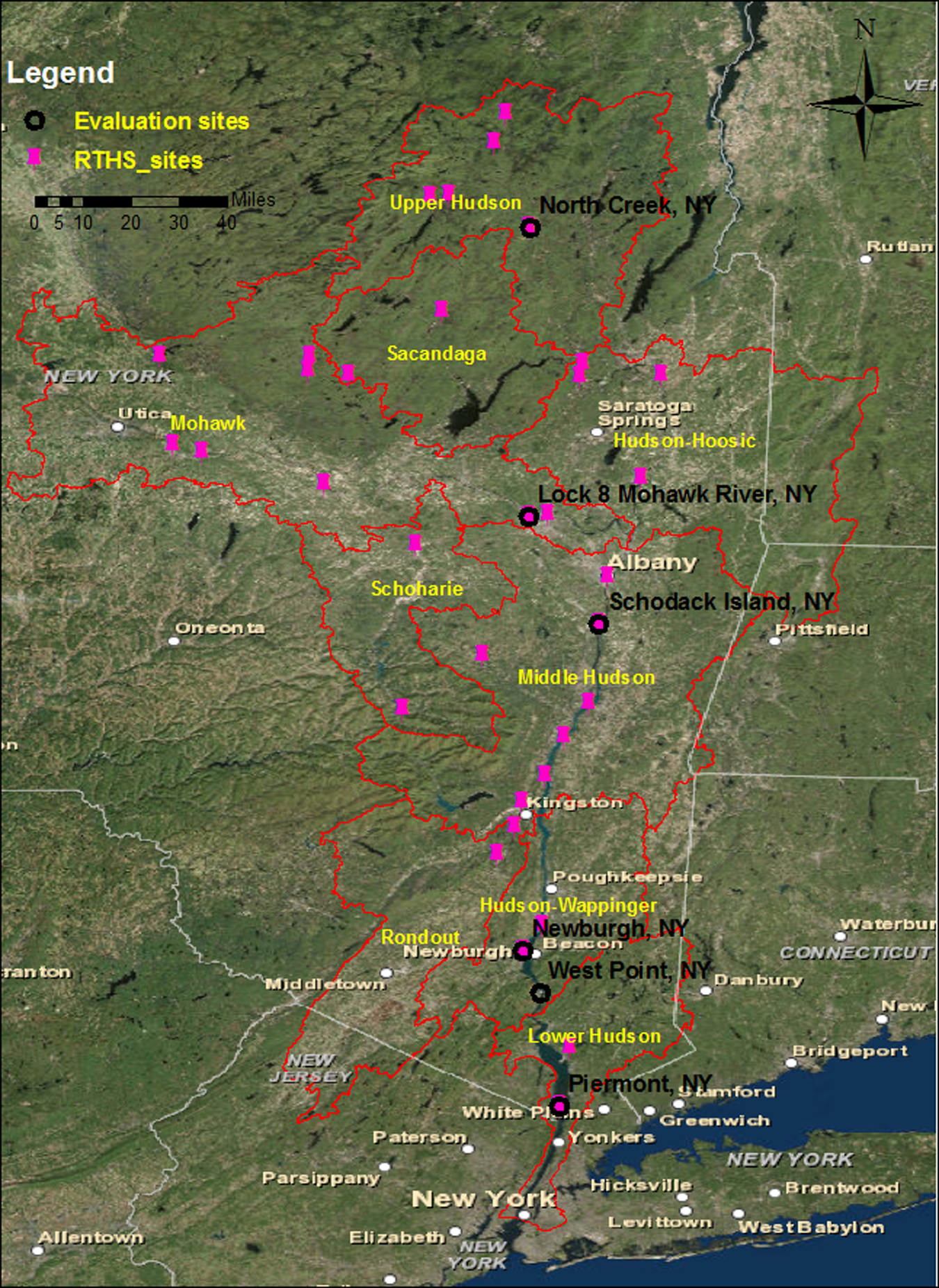
Location of REON RTHSs and field evaluation sites in the Hudson River and Estuary. REON, River and Estuary Observatory Network.

Laboratory testing of the precipitation gauge

Laboratory calibrations were performed to determine pressure transducer responses to known water column heights above the pressure sensor. Coefficients to convert raw 16-bit ADC counts to millimeters of precipitation were determined from linear response curves. Each response curve was generated from five points, where each point represented a water level increase (32.8 mm) from a 1 L addition of room temperature deionized water to the precipitation collection chamber. The output was allowed to stabilize (typically <2 min) before recording the value.

Laboratory testing of the stage height sensor

Load and temperature responses of the stage height sensors (i.e., low range and high range) were evaluated in a laboratory column with an operational depth of 105.75 cm. Load responses of the stage height sensor were recorded at evenly spaced water column depths of 9.75, 33.75, 57.75, 81.75, and 105.75 cm. The sequence of depths was then reversed, and a second set of five depth readings was recorded to check for hysteresis effects. Sensor response coefficients were determined from linear regressions of load responses of the 10 readings. The temperature dependence of the stage height sensor was significant due to the watertight nonvented design and was dominated by changes in internal pressure according to the ideal gas law. The temperature dependence was analyzed by applying a constant load to the sensor, while varying the temperature. This is accomplished by placing the sensor into the bottom of the laboratory column with approximately 1 m of water. The laboratory column with sensor was then placed in a programmable incubator to vary the temperature. The water served as a constant load as well as a buffer to minimize transient temperature effects to observe only absolute temperature effects. The incubator was set to ramp from 5°C to 35°C over 12 h, held at 35°C for 8 h, ramp down to 5°C over 12 h, and then held at 5°C for 8 h. This cycle was performed twice, while monitoring the output of the sensor. A small amount of oil was added to the water chamber to minimize evaporation losses to effectively achieve a constant load.

After correcting for barometric pressure changes, pressure sensor outputs were plotted against the internal sensor temperature to determine the linear temperature response coefficient. Finally, with a known load on the sensor during the temperature calibration, a final offset “C” was calculated. Using the linear load and temperature calibration coefficients and offset, the final equation to convert raw counts (10-bit) to stage height (cm) is

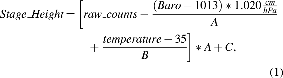
where Stage_Height is level of H₂O above sensor (cm), raw_counts is 10-bit ADC value from pressure transducer, A is linear load calibration coefficient (cm/count), B is linear temperature calibration coefficient (degrees/count), Baro is barometric pressure (hPa), temperature is internal sensor temperature (degrees Celsius) and C is offset (cm).

Field evaluation method of precipitation gauge

The precipitation gauge was field tested from September 2011 to April 2012 to evaluate sensor performance for long-term monitoring. Annual average precipitation at Massena, NY, is 35.0 inches (889 mm) with monthly averages ranging from a maximum of 3.65 inches (92.7 mm) in September and minimum of 1.77 inches (45.0 mm) in February (NOAA, 2016). Thus, the evaluation period spanned the wettest and driest months in northern New York State. The latitude and longitude of the evaluation site were 44.729°N and 74.944°W, ∼24 km from the NOAA station at Massena, NY. The precipitation gauge was field tested in a direct comparison against a colocated NOAH II research-grade precipitation gauge manufactured by ETI Instrument Systems, Inc. The fully factory-calibrated NOAH II precipitation gauge was selected for evaluation purposes as this weighing-type precipitation gauge operates under proven load cell technology, has low power consumption, high accuracy, and advanced digital software filtering technique to reduce errors due to wind, vibration, and other noise sources. Our RTHS and NOAH-II precipitation gauges were mounted at ground level and separated by 3 m in a 1,700 m² field with grassy vegetation reaching a height above grade of ∼1 m. Small trees lined the perimeter of the field, reducing wind effects in the test area. Using an RTHS system, data were simultaneously collected and logged from both precipitation gauges.

To minimize false precipitation reports induced by temperature fluctuations, a software filtering algorithm was developed that applied a minimum precipitation rate threshold of 0.9 mm/h where precipitation rates above the threshold were treated as actual precipitation events and rates below the threshold were assigned a value of 0 mm/h. The threshold value was determined using an optimization routine where the threshold value was adjusted to minimize the occurrence of false events, both positive (i.e., precipitation occurred) and negative (i.e., no precipitation occurred) events. False events were defined as those events recorded by the RTHS gauge when no event was recorded by the reference gauge (NOAH II).

Field evaluation method of stage height sensor

Before field deployments, the stage height sensor response coefficients were determined from sensor responses collected in a calibration column at five evenly spaced water depths between 30.5 cm (1 ft.) and 274.3 cm (9 ft.) (data not shown). The calibrated stage height sensors were then installed at six colocated stage height monitoring sites (Fig. 2, black circles) operated by the USGS, HRECOS, and REON to allow direct comparison of the RTHS stage height performance against the different technologies employed at the various colocated reference stations. Deployment sites included natural riverine systems (North Creek, NY), dam-controlled rivers (Lock 8 Mohawk river, NY), tidal-driven rivers (Schodack Island, NY), and estuarine sections (Newburgh, NY; West Point, NY; Piermont, NY: distinct differences in salinity level among these sites) to evaluate sensor performance under different hydrological, hydrodynamic, and environmental conditions. All RTHS stage height gauges were less than 100 m from colocated gauges, with the exception of North Creek site, where the USGS sensor was located about 500 m downstream.

A review of the USGS (2016) National Water Information System for the three USGS stations evaluated in this study including North Creek (USGS 01315500), Lock 8 Mohawk River (USGS 01354330), and West Point (USGS) lists the use of a “Water-stage recorder and crest-stage gauge.” Although the specific instrumentation used at the USGS sites is unclear, a summary of the different technologies in use at various locations throughout the United States since 1889 is provided by Sauer and Turnipseed (2010). Metadata for the Piermont and Schodack Island sites indicate that gauge heights are determined from barometric pressure-corrected depth readings (i.e., pressure) from YSI6600 multiparameter sondes (HRECOS, 2016a, b). Gauge heights recorded by the REON ADCP at Newburgh are determined from pressure transducer responses that have been corrected for barometric pressure.

As stage height measurements were not referenced to common elevation data (i.e., reported as water surface elevations), data analyses conducted for each colocated sensor pair were based on relative gauge heights with respect to common reference time (i.e., t = 0). The variance in the gauge heights (i.e., water level variation) measured at each colocated sensor pair was used to quantify the accuracy and field merit of the RTHS stage height sensor. The sampling interval of the RTHS gauge was ∼10 s (0.1 Hz). Data intervals reported by the colocated USGS/HRECOS/REON-ADCP reference sensors ranged from 1 min (0.017 Hz) at Newburgh (REON ADCP) to 15 min (0.001 Hz) at North Creek (USGS). Due to variations in sampling intervals, statistical and graphical analyses were performed using the nearest data values, with respect to time, to evaluate relative discrepancies between colocated data sets. The statistical measures include the root mean square discrepancy (RMSD), mean discrepancy, and skill, which are defined by Equations (2 )–(4), respectively.

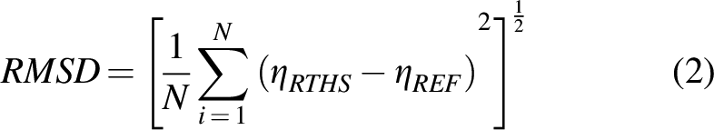
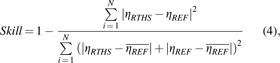
where N is the number of data points, η_REF and η_RTHS are reference and RTHS sensor-measured water level variations over the measurements comparison/validation time period, respectively. Perfect agreement between reference and RTHS sensors gives a skill of 1.0, whereas a complete disagreement gives a skill of 0.0 (Warner et al., 2005).

Results

Laboratory evaluations of the precipitation gauge and stage height sensors were performed throughout their respective developments. The linearity (R²) of the response curves demonstrated the accuracy of each sensor and was an essential element to the design, build, test, and redesign development process. If an RTHS component did not meet the laboratory evaluation criteria, it did not proceed to field evaluation but rather was redesigned, fabricated, and then subjected to a new round of laboratory testing.

Field evaluations of the RTHS demonstrated the reliability and ruggedness of each in-house designed sensor (i.e., precipitation gauge and stage height sensor) and the associated systems. The stage height sensor was subjected to harsh environmental conditions such as 100-year floods and significant ice formation and movement. Inspection of REON records showed 8 stage height sensor faults attributed to mechanical failures and 2 precipitation sensor faults during evaluation periods spanning 105 sensor months (i.e., number of sensors × months of continuous operation).

Laboratory evaluation results of precipitation gauge

Laboratory calibrations of the RTHS precipitation gauge produced correlation coefficients (R²) as high as 0.999 between accumulated precipitation (mm) and raw 16-bit sensors counts, indicating that instrument accuracy was better than 99% (Fig. 3). Calibration was performed at five distinct room temperatures as shown in Fig. 3. Calibration temperature did not significantly affect the linear calibration coefficient (slope of linear regression curve). The y-intercept of the linear regression was attributed to the position of the pressure transducer below the minimum water level in the collection chamber.

FIG. 3.

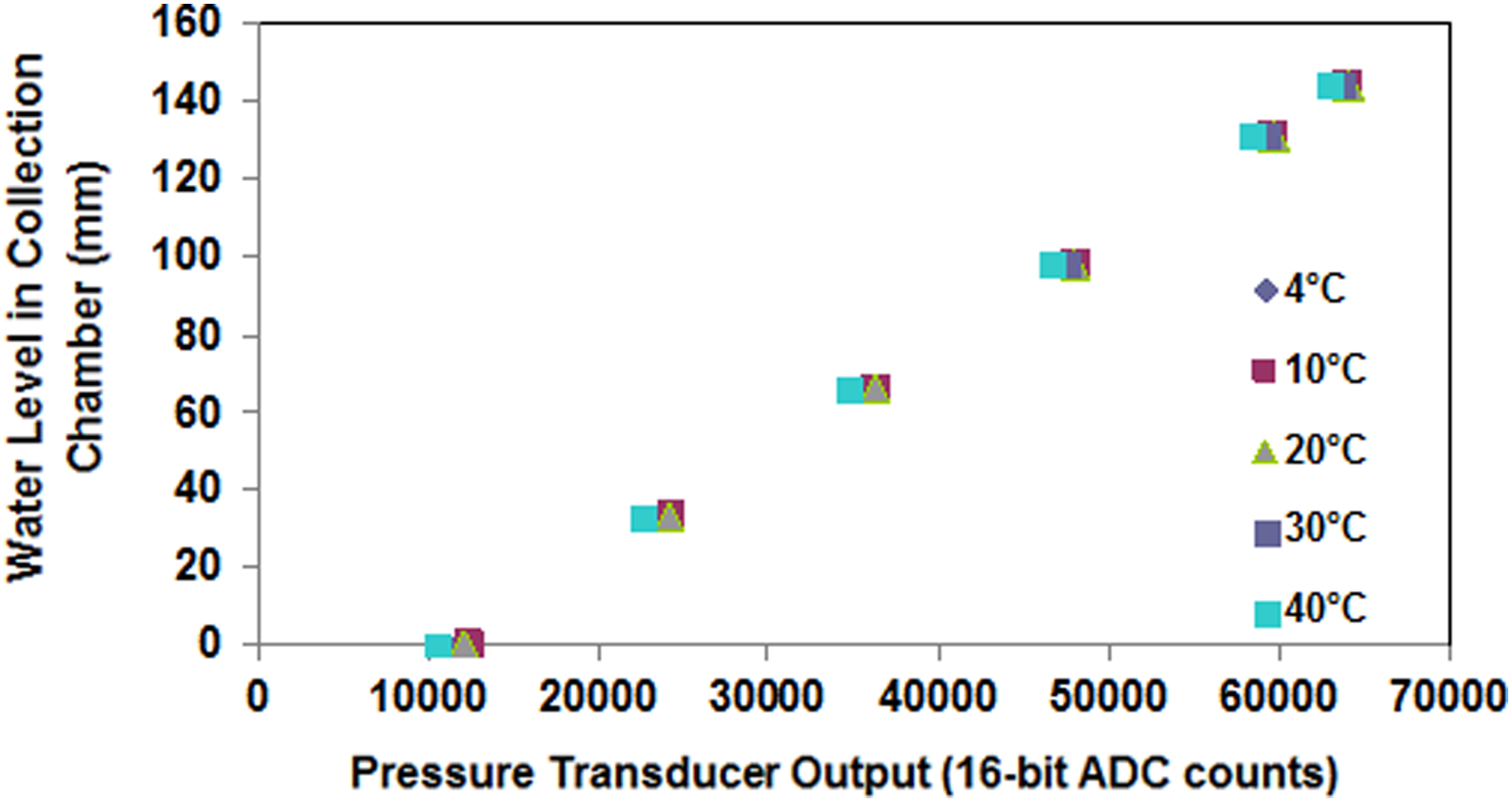
Precipitation calibration performed at five discrete constant temperatures.

The RTHS precipitation sensor includes two pressure transducers to capture low magnitude (<17 mm, total cumulative water level) and large magnitude (<70 cm, total cumulative water level) precipitation events. Laboratory calibrations are indicative of the REON RTHS precipitation gauge's capacity to accurately measure extreme precipitation events up to a maximum accumulated water level of 70 cm (∼27 inches), and is comparable (i.e., 90%) to the capacity specified for the NOAH II gauge. A review of NOAA (2016) precipitation data for station GHCND:USW00094725 located in Massena, NY (44.9358°N 74.8458°W) for the period January 1, 1981–December 31, 2011 shows a maximum daily precipitation of 9.2 cm (3.6 inches), ∼13% capacity of the RTHS gauge, thus demonstrating the ability to the RTHS gauge to capture extreme events in the field.

Laboratory evaluation results of stage height sensor

The stage height sensor laboratory load evaluations produced linear responses for both low- and high-range transducers with R² values of 0.999 (Fig. 4a). For a total of 16 fabricated stage height sensors, the mean response coefficients for the low-range pressure transducer were 0.345 cm/count, standard deviation of 0.023 cm/count, and covariance 6.7%. Evaluation of the high-range transducers gave a mean response coefficient of 1.00 cm/count, standard deviation of 0.007 cm/count, and covariance 0.7%. Similarly, the temperature response coefficients produced linear responses with R² values greater than 0.99 (Fig. 4b) and very low variances between the sensors. The temperature response coefficients determined during this evaluation were applied as calibration coefficients to each sensor before field deployment. The low variance in load and temperature response coefficients demonstrates the reproducibility of the electrical and mechanical designs necessary for high-volume gauge fabrication.

FIG. 4.

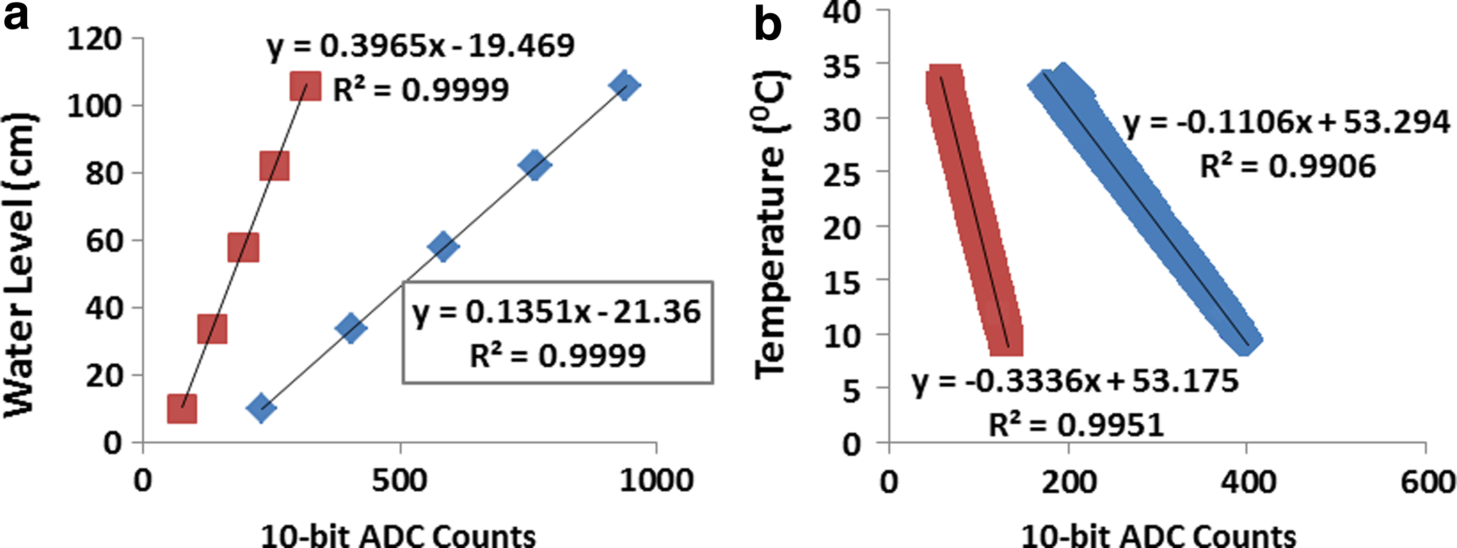
Laboratry evaluation of stage height sensor (a) load, and (b) temperature response. Both high- (red) and low-range (blue) sensors are shown.

Field evaluation results of precipitation gauge

A strong correlation between precipitation measured during 63 events, including liquid and frozen precipitation events between September 2011 and April 2012, with colocated NOAH II and RTHS precipitation gauges was demonstrated with an R² = 0.967 (Fig. 5). Precipitation occurred during each week of the field study. Separate precipitation events were defined using an interevent time of 20 min (Dunkerley, 2008). Over the 126-day study, there were 63 and 53 precipitation events recorded by the RTHS and NOAH II gauges, respectively. In cases where a precipitation event was not captured by the NOAH II gauge, the quantity recorded included trace (i.e., quantitatively equivalent to zero) to less than 1.8 mm of precipitation. The near-zero y-intercept of the linear regression was inconsequential, as daily precipitation below 0.127 mm was considered trace precipitation by the U.S. NWS (U.S. National Weather Service, 1989) and was treated quantitatively as zero (Yang et al., 1998). Where precipitation primarily existed as snow, measurement discrepancies as high as 80% may be attributed to wind (Emerson and Macke-Rowland, 1990; Tabler et al., 1990; Yang et al., 1999; Gordon, 2003). Due to initial abstraction in the watershed, such discrepancies are not expected to significantly affect output of hydrological models, which are routinely used in decision-making processes for water resources management. A review of precipitation data from NOAA (2016) station (GHCND: USW00094725) located in Massena, NY (44.9358°N 74.8458°W) observed at the Massena International Airport for the period September 04, 2011–April 30, 2012 shows a maximum daily rainfall event of 27 mm, which is comparable to maximum rainfall event of 30 mm recorded with both the RTHS and NOAH II gauges (Fig. 5). Although the location of the NOAA station at the Massena International Airport and test sensors is separated by a distance 24 km, the close agreement of maximum rainfall events is indicative of the accuracy of the RTHS measurements.

FIG. 5.

Daily accumulation of RTHS precipitation gauge and NOAH II in 2011–2012.

Field evaluation results of stage height sensor

Field testing the stage height sensor in diverse environmental conditions attests to the ruggedness and adequate performance of the sensor. Figure 6a–d displays water level variations at North Creek (i.e., a representative site at the natural riverine system), Lock 8 Mohawk River (i.e., a representative site at dam-controlled section of the river), Schodack Island (i.e., a representative site at the tidal-driven freshwater section), and Piermont (i.e., a representative site at tidal-driven estuarine section) sites, respectively (see Fig. 2 for the site locations). The red and blue lines represent the RTHS and the reference stage height sensor-measured water level variations, respectively. The black lines denote discrepancies between these two independent measurements. These figures demonstrate the ability of the RTHS gauge to capture dynamic changes in water levels due to tidal and episodic events. Mean discrepancies (Fig. 6, black lines) between the RTHS and reference sensor measurements range between 1.2 and 2.8 cm (Table 2) at all evaluation sites. Discrepancy comparisons at the Newburgh and West Point stations (data not presented) are similar to those observed at Piermont (Fig. 6d).

FIG. 6.

RTHS and reference sensor-measured water level variation and their discrepancies at four sites: (a) North Creek, (b) Lock 8 Mohawk River, (c) Schodack Island, and (d) Piermont. Note: blue, red, and black lines represent RTHS measurements, reference sensor measurements, and their discrepancies, respectively.

Table 2.

Field Performance Statistics of the RTHS Stage Height Sensor

Site location	Secondary measurement	Dates of validation	Number of colocated measurements	Water level change (cm)	Water level comparisons regression statistics	Water level discrepancy statistics
North Creek, NY	USGS site 01315500	Nov 1, 2013 to Nov 30, 2013	2,858	63.1	R² = 0.989	Skill = 0.987
					Slope = 1.03	MD = 2.62 cm
					Intercept = 3.62	RMSD = 2.88 cm
Lock 8 Mohawk River, NY	USGS site 01354330	Oct 18, 2013 to Dec 6, 2013	10,693	151.8	R² = 0.999	Skill = 0.999
					Slope = 1.01	MD = 1.2 cm
					Intercept = 0.84	RMSD = 1.44 cm
Schodack Island, NY	HRECOS site hydrological station	Oct 18, 2013 to Nov 18, 2013	3,053	228.3	R² = 0.999	Skill = 0.999
					Slope = 1.0	MD = 1.66 cm
					Intercept = 0.91	RMSD = 2.09 cm
Newburgh, NY	REON ADCP	Sep 8, 2013 to Sep 14, 2013	9,911	133.3	R² = 0.998	Skill = 0.998
					Slope = 1.03	MD = 2.66 cm
					Intercept = 1.51	RMSD = 3.21 cm
West Point, NY	USGS site 01374019	Nov 13, 2013 to Nov 30, 2013	1,637	193.5	R² = 0.999	Skill = 0.998
					Slope = 1.01	MD = 2.77 cm
					Intercept = 2.93	RMSD = 3.11 cm
Piermont, NY	HRECOS Piermont pier hydrological station	Nov 13, 2013 to Nov 23, 2013	968	164.9	R² = 0.999	Skill = 0.999
					Slope = 1.01	MD = 1.51 cm
					Intercept = 0.84	RMSD = 1.81 cm

HRECOS, Hudson River Environmental Conditions Observation System; MD, mean discrepancy; REON, River and Estuary Observatory Network; RMSD, root mean square discrepancy.

Inspection of the hydrographs (Fig. 6) shows maximum observed stage variabilities on the order of 2 m. Considering the 3.5 m maximum detection limit of low-range sensor with the requirement that stage gauge installations be below the minimum expected water levels implies the need for the high-range sensor to fully characterize extreme stage heights. Furthermore, the ability of the high-range sensor to accurately measure relatively small changes in water levels, as indicated in laboratory evaluations, suggests the adequacy of the high-range sensor in systems where the water levels are relatively static. However, evaluations of the sensor response coefficients indicate that the low range sensor is suitable for applications where measurement resolutions less than 1 cm are required. Although the added value of the second pressure transducer is not demonstrated by the field evaluations presented herein, redundant measurements are applicable to data quality assurance programs and improved network reliability during extreme events when stage height measurements are most critical.

Synchronizing the RTHS and reference sensor measurements provides further insights into the accuracy of the RTHS stage height sensor measurements. Relative discrepancies among these data sets are assessed using statistical and graphical analyses. Table 2 lists time periods of colocated measurements and various statistical measures of these discrepancies at six sites. Statistical analysis of measured data sets at the six sites further demonstrates the strong correlation between the RTHS and reference sensor measurements, with R² ranging from 0.989 to 0.999 and RMSDs ranging from 1.4 to 3.2 cm. The slope of the linear regression curves (ranges from 1.00 to 1.03) and the calculated “skill” value (range 0.987–0.999) further demonstrate excellent agreement between the RTHS and reference sensor measurements and attest to the accuracy of the RTHS sensor. Figure 7 displays graphical comparisons of the RTHS and reference sensor measurements at four sites (e.g., North Creek, Lock 8 at Mohawk River, Schodack, and Piermont). The open circles in Fig. 7 represent measured water level changes, whereas the black and red lines denote the linear regression and the 1:1 line between the RTHS and reference sensor measurements. RTHS stage height sensor measurements at Lock 8, Schodack, and Piermont sites are almost in perfect agreement with reference sensor measurements at the same locations, although some occasional discrepancies are apparent in the Schodack data that are coincident with anomalous RTHS and HRECOS stage height observations.

FIG. 7.

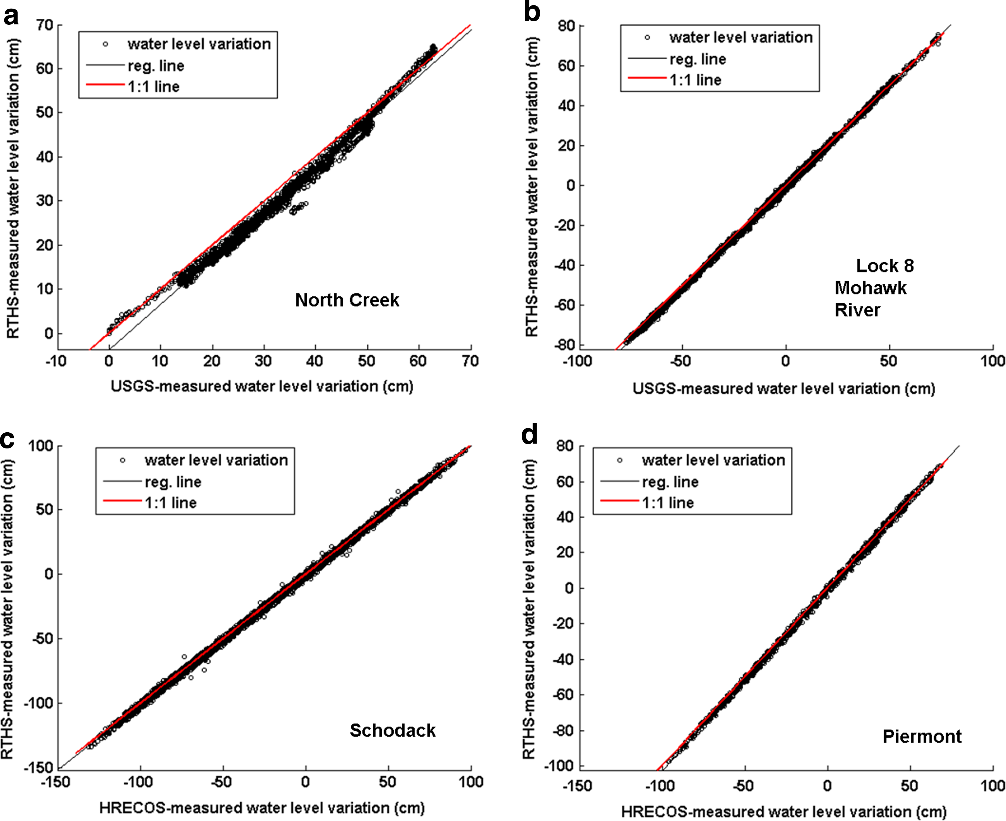
Comparison of RTHS and reference sensor measurements at four sites: (a) North Creek, (b) Lock 8 Mohawk River, (c) Schodack Island, and (d) Piermont. Note: black open circles, black and red lines represent water level measurements, linear regression of these measurements, and hypothetical perfect match of these measurements (1:1 line, i.e., RTHS-measured water level change = reference sensor-measured water level changes), respectively (see Table 2 for comparison statistics).

One instance of the anomalies observed at Schodack is critically analyzed in Fig. 8, where red and blue circles represent the RTHS and HRECOS water level changes, respectively. The two data sets were independently collected, suggesting that the anomalies were not a sampling or systemic error. The anomalous event was evident in both data sets but was more clearly observed in the RTHS data sets due to higher sampling frequency (10 s) compared with the HRECOS reporting frequency (15 min). To evaluate whether the anomaly was false, the 15-min HRECOS (2016a) data were compared against the 5-min average RTHS (http://rths.us) data. Coincident data points (i.e., on the 15-min interval) showed the anomaly, with essentially the same time series profiles in both systems (data not shown) at 09:15 EST on November 7, 2013. Application of Equation (4) to the data set for the period 08:00–09:45 EST gave a skill value of 0.966 that was indicative that the observed anomaly was a real event. Inspection of the RTHS data (5-min average) at 09:10 and 09:20 EST showed water levels in line with normal tidal variations, which indicated that the anomalous readings occurred within the RTHS 5-min averaging interval. Although characterizing the cause of the anomalous water level is beyond the scope of this study, its prominence in the high resolution RTHS data set demonstrates the value of high frequency measurements (i.e., short sampling intervals) to characterize ephemeral environmental processes.

FIG. 8.

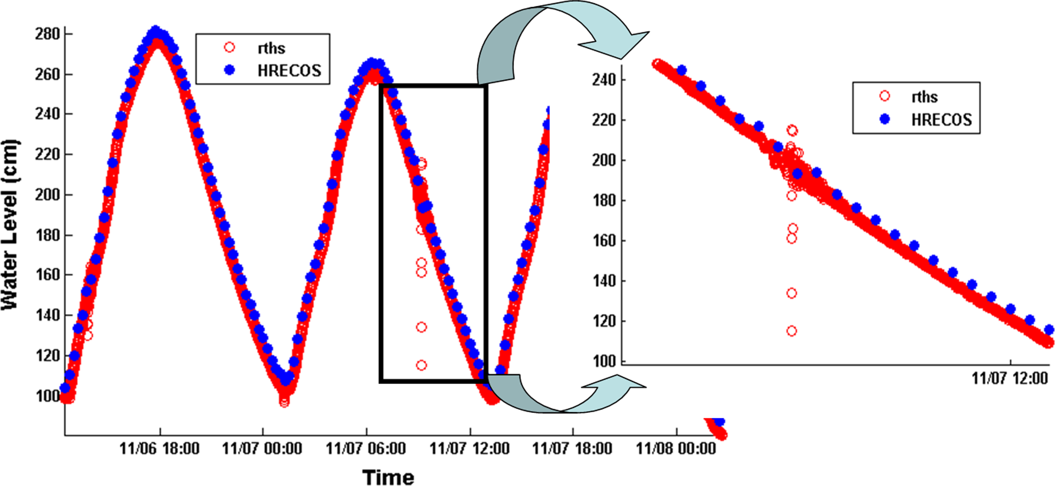
RTHS and HRECOS gauge measurements versus time at Schodack Island. The inset plot highlights one instance of data anomaly. HRECOS, Hudson River Environmental Conditions Observation System.

Discussion

The RTHS has been designed, developed, fabricated, and tested in the laboratory and the field. Results of laboratory testing of the precipitation gauge and stage height sensor demonstrated promising accuracy and precision with response curves giving R² as high as 0.999. In the field, both sensors performed well in terms of reliability, and compared well against colocated research-grade sensors. The precipitation gauge field testing occurred during events of both liquid and solid precipitation, demonstrating its all-season capability. Similarly, the stage height sensor field testing occurred in diverse aquatic systems throughout the summer and winter, demonstrating its ruggedness and reliability.

Field testing the in-house designed precipitation gauge sensors included a direct comparison with an NOAH II precipitation gauge. Despite the potential for wind-induced errors during snowy conditions, a 5.8% difference between the sensors was demonstrated during the evaluation period with total liquid equivalent precipitation amounts of 312 and 330 mm, for the RTHS and NOAH II gauges, respectively. World Meteorological Organization (2008) also reported that aerodynamic properties of precipitation gauges can limit measurement uncertainty to the largest of 5% or 0.1 mm for daily accumulations. Adequate performance of the RTHS precipiation gauge was indicated by comparable variabilities of 5–13% for identical and colocated precipitation gauges (Ciach, 2003; Basara et al., 2009). A slight measurement bias is indicated in Fig. 8, where RTHS values were ∼94% of the NOAH II values. This bias may have been attributed to separate and independent factory and laboratory calibrations for the NOAH II and RTHS gauges, respectively. Measurement errors due to precipitation undercatch associated with the diameter of the gauge orifice have been reported (Gordon, 2003). Thus, the smaller diameter of the RTHS gauge (19.7 cm) when compared with the NOAH II (30.2 cm) may have contributed to the observed bias. However, this bias would have been insignificant in comparison with inherent spatial and detection variability associated with all types of precipitation gauge measurements. For example, DeWalle and Rango (2008) reported that identical and colocated precipitation gauges measure different precipitation amounts depending on many factors, including precipitation states (solid, liquid, size of precipitation drops, etc.), wind speed and direction, turbulence, and sublime precipitation. Long-term bias was much smaller than the effects of these variabilities on precipitation measurements (Ciach, 2003; Basara et al., 2009).

The RTHS and USGS stage height measurements at North Creek displayed the highest relative discrepancies of the six sites evaluated (Fig. 6a) as indicated by the greatest deviation from a 1:1 line of the two-stage height measurements (Fig. 7a). These deviations were likely due to variations in cross section geometries (width, depth, etc.) at two locations. Specifically, the stream widths of the RTHS and the USGS stage height sensors in North Creek were 120 and 80 m, respectively. Thus, the channel cross section at the RTHS gauge was less confined than the channel at the USGS gauge. Assuming that flow was equal at both stations, as supported by the lack of tributary intersections between two stations, suggests that the measured stage height variations would have been less at the RTHS gauge in comparison with the USGS gauge, especially when the flow remained confined to the main channel (i.e., at low flows). At the higher stream stage heights (i.e., >50 cm, Fig. 6a), there was little observed difference between the two gauges and indicated the possibility of pooling upstream of the channel constriction at the USGS station. Occasional discrepancies between the RTHS and HRECOS measurements were observed at Schodack and attributed to different sampling rates (Fig. 7c). Although characterizing the cause of the stage height anomalies is beyond the scope of this study, RTHS measurements demonstrate the need for high-freqeucny sampling to fully characterize the magnitude of these transient signals (Fig. 8).

Field testing results demonstrate the viability of RTHS as a low-cost alternative, with adequate and comparable performance, to commercially available sensor systems. The RTHS costs an order of magnitude less than commercially available weather stations and stage height sensors, which are capable of real-time measurements and dissemination of the same parameters. The cost of an USGS stage height sensor varies depending on the type of stage height sensor installed. Cost estimates to install a new stilling well with a float sensor or bubble gauge with a nonsubmersible pressure transducer vary between $30,000 and $50,000 (Mui et al., 2010) compared with less than $1,000 for an RTHS stage height sensor. The cost difference is less extreme when comparing the RTHS with one that uses a submersible pressure transducer or noncontact-type stage sensor (acoustic, radar, and optical methods) (Mui et al., 2010; Sauer and Turnipseed, 2010). In stilling well float-driven sensor systems, high capital costs are due to the installation (i.e., construction) of a stilling well with sufficient depth for its bottom has to be at least a foot below the minimum stage anticipated and a height above the level of a 2% annual exceedance probability (50 year) flood (0.5% annual exceedance probability [200 years] flood for NSIP stream gauges). Moreover, a standard USGS stilling well requires inside dimensions of 4 ft diameter or width. Additional costs are required for flushing systems or silt trap to prevent clogging of stilling well intake pipes (Sauer and Turnipseed, 2010). The high costs of bubble gauges with nonsubmersible pressure transducers are due to the requirement for gas-purge systems and stilling well installations.

In comparison, the RTHS stage height sensor is relatively simple, requiring only a metal pipe for mounting with a single power/data connection through a submersible cable. Use of barometric pressure correction algorithms translates to reduced capital cost by alleviating the need for expensive vented cables and cable terminals. Considering the simpler design and reduction in physical infrastructure requirements, our analysis shows the RTHS stage height sensor to be more cost effective than either the stilling well or gas-purge systems. Noncontact-type water level sensors (acoustic, radar, and optical methods) have the potential to reduce the costs significantly in future. However, they are still in development stage and some are not yet able to achieve USGS accuracy standards.

The developed RTHS demonstrates the viability of combining systems to measure meteorological and hydrological parameters in a comprehensive monitoring network with shared physical and cyber infrastructures. This merging of services by a single observatory has the potential to significantly reduce the cost per unit data. Such reductions are necessary to address budgetary constraints that pose threats to the sustainability and expansion of long-term hydrological monitoring programs required to support resource management decisions and scientific initiatives.

Conclusion

The RTHS has been designed and evaluated for use as a hydrological monitoring tool. Laboratory evaluations of the RTHS precipitation gauge and stage height sensors demonstrated adequate accuracy and precision with correlation coefficients (R²) as high as 0.999. Field evaluations also demonstrated the reliability and ruggedness of each in-house designed sensor (i.e., precipitation gauge and stage height sensor) and the associated systems. The RTHS stage height sensor measurements showed excellent agreement with the USGS/HRECOS/REON research-grade sensor measurements at six colocated sites with mean discrepancies and “skill” values ranging from 1.2 to 2.77 cm and from 0.987 to 0.999, respectively. Analysis of high-frequency stage height measurements demonstrated the capacity of the RTHS gauge to capture dynamic water level changes during episodic events when water level can change dramatically over a short time interval.

Modular RTHS design allows system upgrades with faster, less expensive, more efficient, and reliable components borne through enabling technology developments. The modular design also enables expansion of sensor types (water quality and meteorological sensors [e.g., solar radiation, snow depth, soil moisture, and evaporation rate]), which can further reduce unit data cost. The integration of other low-cost water quality sensors (e.g., pH, turbidity, and dissolved oxygen) into the RTHS is currently undergoing field performance evaluations. Another RTHS upgrade under consideration is a remote/automatic precipitation gauge drain to maximize the station service intervals (i.e., reduced maintenance costs). Through continued implementation of proven technology and interactive system refinement, the RTHS system represents an affordable option for water resources monitoring professionals requiring an accurate real-time monitoring system.

Footnotes

Acknowledgments

Funding for this work was provided by the Beacon Institute for Rivers and Estuaries at Clarkson University and the National Science Foundation (grant nos. CBET-1058422 and CBET-0821531). Thanks go to the REON field engineering team, especially Patrick O'Brien, William Kirkey, and Russ Nelson for their support in the data collection effort.

Author Disclosure Statement

No competing financial interests exist.

References

Andreassian

, Perrin

, Michale

, Usart-Sanchez

, and Lavabre

(2001). Impact of imperfect rainfall knowledge on the efficiency and the parameters of wateshed model. J. Hydrol., 250, 206.

Barnett

T.P.

, Adam

J.C.

, and Lettenmaier

D.P.

(2005). Potential impacts of a warming climate on water availability in snow dominated regions. Nature. 438, 303.

Basara

J.B.

, Illston

B.G.

, Winning

T.E.

, and Fiebrich

C.A.

(2009). Evaluation of rainfall measurements from the WXT510 Sensor for use in the Oklahoma City Micronet. Open Atmos. Sci. J., 3, 39.

Becker

, Schiebelsberger

, Weber

, Vodermayer

, Zehner

, and Kummerle

(2006). An Approach to the Impact of Snow on the Yield of Grid Connected PV Systems. Munich: Bavarian Association for the Promotion of Solar Energy.

Ciach

G.J.

(2003). Local random errors in tipping-bucket rain gauge measurements. J. Atmos. Oceanic Technol., 20, 752.

DeWalle

, and Rango

(2008). Principles of Snow Hydrology. New York: Cambridge University Press.

Dunkerley

(2008). Identifying individual rain events from pluviograph records: A review with analysis of data from an Australian dryland site. Hydrol. Process., 22, 5024.

Emerson

D.G.

, and Macek-Rowland

K.M.

(1990). Solid-precipitation (snowfall) measurement intercomparison, Bismarck, North Dakota. U.S. Geological Survey, Open-File Report 90–124.

Gilbert

(2010). A dearth of data on water resources is holding up improved management practices. Nature. (published online 4 Oct. 2010) DOI: 10.1038/news.2010.490.

10.

Gordon

J.D.

(2003). Evaluation of candidate rain gauges for upgrading precipitation measurement tools for the national atmospheric deposition program. U.S. Geological Survey, Water-Resources Investigations Report 02–4302.

11.

Harmancioglu

N.B.

, and Alpaslan

(1992). Water quality monitoring network design: A problem of multi-objective decision making. J. Am. Water Res. Assoc., 28, 179.

12.

HRECOS. (2016a). Hudson River Environmental Conditions Observing System. Schodack Island Hydrologic Station data. Available at: www.hrecos.org/ (accessed July 24, 2016).

13.

HRECOS (2016b). Hudson River Environmental Conditions Observing System. Piermont Pier Hydrologic Station data. Available at: www.hrecos.org/ (accessed July 24, 2016).

14.

Hubbart

, Link

, Campbell

, and Cobos

(2005). Evaluation of a low-cost temperature measurement system. Hydrol. Process., 19, 1517.

15.

Huntington

T.G.

(2006). Evidence for intensification of the global water cycle: Review and synthesis. J. Hydrol., 319, 83.

16.

Jackson

R.B.

, Carpenter

S.R.

, Dahm

C.N.

, McKnight

D.M.

, Naiman

R.J.

, Postel

S.L.

, and Running

S.W.

(2001). Water in a changing world. Ecol. Applic., 11, 1027.

17.

Jordan

(2000). Sampling errors in radar estimates of rainfall. J. Geophys. Res. Atmos., 105, 2247.

18.

Maidment

D.R.

(1993). Handbook of Hydrology. New York: McGraw-Hill, Inc.

19.

Montgomery

J.L.

, Harmon

, Haas

C.N.

, Hooper

, Clesceri

N.L.

, Graham

, Kaiser

, Sanderson

, Minsker

, Schnoor

, and Brezonik

(2007). The WATERS network: An integrated environmental observatory network for water research, Environ. Sci. Technol., 41, 6642.

20.

Mui

C.K.

, Royem

A.A.

, and Walter

M.T.

(2010). Low-Cost Stream Gaging Through Analysis of Stage Height Using Digital Photography, AGU Fall Meeting (Abstract No. H51D- 0930). San Francisco, CA. Available at http://adsabs.harvard.edu/abs/2010AGUFM.H51D0930M (accessed July 15, 2016).

21.

NOAA. (2016) National Climate Data Center. Available at: www.ncdc.noaa.gov/cdo (accessed June 24, 2016).

22.

Parry

M.L.

, Canziani

O.F.

, Palutikof

J.P.

, van der Linden

P.J.

, and Hanson

C.E

. eds. (2007). Climate Change 2007: Impacts, Adaptation and Vulnerability. Contribution of Working Group II to the 4th Assessment Report of the Intergovernmental Panel on Climate Change. Cambridge, U.K.: Cambridge University Press.

23.

Piasecki

, Ames

, Goodall

, Hooper

, Horsburgh

, Maidment

, Tarboton

, and Zaslavsky

(2010). Development of an Information System for the Hydrologic Community, 9th International Conference on Hydroinformatics (HIC 2010). Tianjin, China.

24.

Raghunath

H.M.

(2006). Hydrology: Principles, Analysis and Design. New Delhi: New Age International. 2006- Hydrology, p. 476.

25.

Revenga

, Campbell

, Abell

, de Villiers

, and Bryer

(2005). Prospects for monitoring freshwater ecosystems towards the 2010 targets. Phil. Trans. R. Soc. Lond. B., 360, 397.

26.

Sauer

V.B.

, and Turnipseed

D.P.

(2010). Stage Measurement at Gaging Stations. U.S. Geological Survey Techniques and Methods Book 3, Chapter A7, p. 45. Available at http://pubs.usgs.gov/tm/tm3-a8/ (accessed July 15, 2016).

27.

Schuurmans

J.M.

and Bierkens

M.F.P.

(2007). Effect of spatial distribution of daily rainfall on interior catchment response of a distributed hydrological model. Hydrol. Earth Syst. Sci., 11, 677.

28.

Tabler

R.D.

, Berg

N.H.

, Trabant

D.C.

, Santeford

H.S.

, and Richard

P.A.

(1990). Measurement and evaluation of winter precipitation. In Ryan

W.L.

and Crissman

R.D.

, Eds., Cold Regions Hydrology and Hydraulics Monograph. New York: American Society of Civil Engineers, pp. 9–38.

29.

U.S.G.S. (2016). National Water Information System: Web Interface. Available at: http://waterdata.usgs.gov/nwis/rt (accessed June 24, 2016).

30.

U.S. National Weather Service. (1989). Cooperative Station Observations NWS Observing Handbook No. 2. Silver Spring, MD. Available at http://www.nws.noaa.gov/os/coop/Publications/coophandbook2.pdf (accessed July 15, 2016).

31.

Villarni

, Mandapaka

P.V.

, Krajewski

W.F.

, and Moore

R.J.

(2008). Rainfall and sampling uncertainties: A rain gauge perspective. J. Geophys. Res., 113, D11102.

32.

Vladisauskas

, and Jakevivius

(2004). Absorption of Ultrasonic waves in Air, Ultragaesas, Nr.1(50), ISSN 1392–2114.

33.

Wang

, Xie

, Sharif

, and Zeitler

(2008). Validating NEXRAD MPE and Stage III precipitation products for uniform rainfall on the upper Guadalupe river basin of the Texas Hill Country. J. Hydrol., 348, 73.

34.

Warner

J.C.

, Geyer

W.R.

, and Lerczak

J.A.

(2005). Numerical modeling of an estuary: A comprehensive skill assessment. J. Geophys. Res., 110, C05001.

35.

World Meteorological Organization. (2008). Guide to Meteorological Instruments and Methods of Observation. Available at https://www.wmo.int/pages/prog/gcos/documents/gruanmanuals/CIMO/CIMO_Guide-7th_Edition-2008.pdf (accessed July 15, 2016).

36.

Yang

, Goodison

B.E.

, and Metcalfe

J. R.

(1998). Accuracy of NWS 8″ standard nonrecording precipitation gauge: Results and application of WMO intercomparison. J. Atmos. Oceanic Technol., 15, 54.

37.

Yang

, Goodison

B.E.

, Metcalfe

J.R.

, Louie

, Leavesley

, Emerson

, et al. (1999). Quantification of precipitation measurement discontinuity induced by wind shields on national gauges. Water Resour. Res., 35, 491.