




Abstract
Abstract
A hierarchical modeling approach was used to diagnose the variability of U.S. wastewater treatment facility compliance with existing discharge permit limits. The first level of hierarchy modeled monthly variability in treated water quality over a 4-year period using a Generalized Linear Model, which relates compliance to plant characteristics such as flow rate, capacity utilization, seasonality, and compliance history. Residuals from this model were subjected to a spatial analysis using Kriging in the second level of hierarchy to model spatial covariability. This hierarchical approach was used for three effluent constituents: biochemical oxygen demand (BOD), total suspended solids (TSS), and ammonia, in discharge monthly report data for the period 2004–2008 from a random sample of more than 100 municipal plants. The first level of hierarchy captured most of the total variance in compliance data for all three pollutants. Seasonality was seen to affect effluent concentrations of BOD and TSS, which have uniform national discharge standards, but not ammonia, for which permit limits are typically seasonal. Levels of compliance for BOD, TSS, and ammonia all were significantly affected by the respective effluent concentration in the previous month. The second level of hierarchy identified geographic regions of anomalous compliance and improved the model's predictive performance for a subset of plants with discharges closer to permit limits.
Introduction
H
However, the ability to evaluate compliance with NPDES limits on a regional or national scale is of increased interest for understanding the actual impacts of wastewater discharges on water quality and for assessing the effects of changes in discharge regulations. Of particular importance is adoption of more stringent discharge limits for nutrients, which has increased in pace since 1998 (Fig. 1). In 1998, 39 states and the District of Columbia had no numeric water quality criteria for nutrients that covered all of a particular type of water body, for example, lakes, rivers/streams, estuaries, and coastal waters, and only three states had numeric criteria applied to all of one or two water types; only one state, Hawaii, had statewide numeric nutrient criteria for all water types. The United States Environmental Protection Agency (USEPA) expects an increasing trend in statewide regulation of nutrients by water body type, anticipating that by 2016 nine states will have numeric criteria for nitrogen species and/or phosphorus for all of one or more water types, and at least two states will regulate both nutrients for all water types.

Progress in specifying water quality criteria for nitrogen species and/or phosphorus by 50 states and the District of Columbia, 1998–2016. [USEPA 2015 www.epa.gov/nutrient-policy-data/state-development-numeric-criteria-nitrogen-and-phosphorus-pollution].
In light of the increase in broad water quality criteria for nutrients, the ability to evaluate compliance with NPDES limits on a regional or national scale is of increased interest for understanding the actual impacts of wastewater discharges on water quality and for assessing the effects of changes in discharge regulations. Of particular importance is adoption of more stringent discharge limits for nutrients, which has increased in pace since 1998 (Fig. 1). In 1998, 39 states and the District of Columbia had no water quality criteria for nutrients and only three states had criteria applied to all of one or two water types; only one State, Hawaii, had comprehensive nutrient criteria for all water types. The USEPA has anticipated that by 2016 nine states will have criteria for nitrogen species and/or phosphorus for all of one or more water types, and two states will regulate both nutrients for all water types.
In 2012, the USEPA estimated costs and benefits of uniform national regulations for nitrogen and phosphorus discharges and reported that capital cost of added technology (retrofitting, new installation) could exceed $50 billion, ($5 to $63/capita/year) with annual operating costs more than $5 billion. The burden on small utilities would be even greater given the diseconomies of scale for small systems. Furthermore, the cost of developing and obtaining approval for the new regulation would exceed $10 million and take at least 5 years (Shapiro, 2012). In states considering new water quality criteria and associated nutrient discharge regulations, the local stakes are also significant. Certainly, water quality degradation is an important result of noncompliance, and enforcement actions also carry significant costs to regulators, utilities, and ratepayers. A few researchers have studied the potential for compliance with emerging limits for nutrients. Daigger et al. (2014) used data from 30 mechanical wastewater treatment plants and 23 lagoon facilities in Utah to predict compliance with more stringent discharge standards for nitrogen and phosphorus, using a spreadsheet-based process simulator. They found that plant capacity was an important determinant of the ability of facilities to meet higher levels of nutrient removal, with the greatest performance and cost impacts on small plants.
A recent approach to evaluate the aggregate performance of wastewater treatment facilities is based on national compliance data and selected plant characteristics in a statistical model. The motivation for this is to develop a decision support tool for planning and regulatory agencies considering systemic issues such as changes to water quality-based effluent limits and enhanced monitoring of discharge permit compliance. A generalized linear model (GLM) was used to predict the probability of meeting permit standards as a function of the degree of decentralization of wastewater systems, which is associated with individual plant capacity since decentralized collection and treatment inherently consist of smaller facilities serving a given population. Four years of discharge monthly reports (DMRs) from 200 treatment plants in the USEPA Integrated Compliance Information System (ICIS) database were modeled to predict the likelihood that plants would meet discharge limits for biochemical oxygen demand (BOD), total suspended solids (TSS), ammonia, and fecal coliform based on design capacity and the extent of capacity utilization (Weirich et al., 2011). In a follow-up study using the same data set, prior exceedance of permit limits at a plant was found to be associated with increased probability of subsequent violations when the reported effluent concentration exceeded discharge limits for the same constituent in the previous month (Weirich et al., 2015).
Although Weirich et al.'s (2011) model was a novel statistical initiative to model the current state of national compliance as a function of plant size and operation, there may be many other factors affecting compliance. We hypothesize that national compliance can be best modeled using two different sets of covariates—large scale covariates, which remain fairly constant over space, and local variables, which affect compliance on a smaller scale. These two distinct categories of variables are modeled successively in a hierarchical framework. The first level of hierarchy consists of regression modeling using GLM, where compliance is modeled as a function of plant capacity (flow) and hydraulic loading (similar to Weirich et al.'s 2011 model). In addition, we introduce covariates for seasonality (to test for seasonal variation in treatment performance) and lag (to account for temporal dependence or “persistence” in the discharge water quality data). The second level of hierarchy models spatial variations in compliance. Geographic factors such as temperature, precipitation, and water use may affect municipal wastewater characteristics and also treatment conditions on a local scale. In addition, discharge limits, notably for ammonia, are typically based on local surface water quality standards, which may have a spatial characteristic depending on factors such as in-stream dilution, aquatic life, and designated uses. Another component of compliance data may be associated with location, namely local water quality criteria and associated discharge permit limits for nutrients, particularly ammonia, which is currently the most commonly regulated nutrient. All of these spatial factors together are incorporated using Kriging, using the residuals from the GLM. Both these tiers together model the temporal and spatial variability in discharge compliance over the United States.
Methods
The GLM regression and Kriging procedures, the models in the two levels of hierarchy, are described hereunder.
Generalized linear model
The GLM provides a more flexible approach to regression than a standard linear regression model. In the GLM, the response variable, Y, can be determined by any distribution in the exponential family, whereas standard linear models require observations to be from a normal distribution. Effluent water quality measurements are always non-negative and typically positively skewed, which violates the normality assumption and thus cannot be accurately modeled using a standard linear model. Assuming a binomial distribution for the response variable reduces the GLM to a logistic regression; a Poisson distribution makes it a Poisson regression model, etc. (McCullagh and Nelder, 1989). The ability to model data using a variety of distributions is the major advantage of GLM.
The GLM relation is represented as follows:
where G(.) is any distribution from the exponential family. A link function, η, relates the expected value of Y, and consequently θ, as a linear function of independent variables (or covariates or predictors),
where η (.) is the link function,
The residuals ɛ = Y - E(Y) are assumed to be normally distributed and uncorrelated as with standard linear regression.
The response variables, Y, in this application are the discharge levels of BOD, TSS, and ammonia, normalized to individual facility permit limits to allow comparability on the basis of likelihood of meeting (or violating) permit limits. Values of Y are positive and highly skewed so a Gamma distribution is appropriate and it has three possible link functions (McCullagh and Nelder, 1989)—identity, log, and the canonical link function, inverse.
The GLM relations resulting from the inverse, identity, and log link functions are as shown, hereunder, respectively,
The maximum likelihood method is employed for estimating the model parameters
where k is the number of free parameters to be estimated, n is the number of observations, and L is log of the likelihood function of the model.
Kriging
The second level of hierarchy consists of a spatial model of the average value of residuals at each location, calculated from the first level GLM described previously. Kriging is a spatial interpolation technique where the estimate at any location is the weighted combination of all the observations and is a best linear unbiased estimator (Krige, 1951; Cressie, 1990). A brief description is provided hereunder; however, for details we refer the readers to the references cited in this section.
Consider observations
such that
where wi are the non-negative weights obtained by minimizing the mean squared error:
Equation (9) reduces to
is the covariance vector of the value at the desired location and all the observations. C00 is the observational variance.
The covariance estimates in the said matrix and vectors are obtained by a variogram—which is a function that decays with distance. This is the central aspect of Kriging. A theoretical variogram is fitted to this empirical variogram; exponential dependence is the commonly used model, which embodies the concept that points nearby have high correlation that weakens with distance, and is given by:
where h = si-sj, C0 is the nugget effect caused by dissimilarity of sample values corresponding to points in the vicinity of one another, a is the effective range or the distance at which the variogram reaches its plateau, and C0+C1 is the sill or the maximum variogram value. The range and sill are the two parameters of the variogram that are estimated from the observations. With the appropriate variogram,
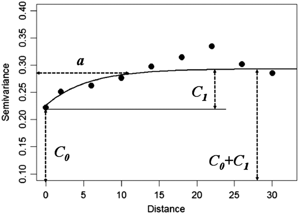
A sample variogram, showing the range a, the nugget effect C0, and the sill C0+C1.
Then the constrained minimization problem is solved using Lagrange multipliers, a standard method for solving such optimization problems (Bivand et al., 2013), and the weights
with the Lagrange multiplier
The variance of the Kriging estimate (i.e., standard error) is obtained from the equation by substituting the expression for
Thus Kriging provides the estimate and the corresponding variance. Fitting an appropriate variogram is generally the difficult part of Kriging as the theoretical options are limited and the data often do not confirm to these options (Bivand et al., 2013). Variations of the said Kriging method, also known as Ordinary Kriging, have been proposed to incorporate external variables in addition to distance (Bivand et al., 2013).
Kriging is an attractive and easy-to-implement method to model spatial fields especially if the data are irregularly spread out in space. The advantages of Kriging include the ability to assign weights based on its proximity to the point of estimation. Kriging also helps compensate the effect of data clustering, by considering points in a cluster as a single point. In our study, the plant locations are clustered at some regions and this makes Kriging the more suitable spatial interpolation technique. Also, during the estimation process, Kriging provides uncertainty estimates that can be helpful for mapping estimation error or for simulation of Kriging estimates. Kriging has found wide applications in various domains, including average monthly temperature interpolation studies (Wu and Li, 2013), groundwater nitrate pollution studies (Chica-Olmo et al., 2014), and river pollution in tidal streams (Chen et al., 2012). The hierarchical modeling approach already described is finding variety of applications, for example, in blending observed and satellite precipitation data (Verdin et al., 2015a), stochastic space–time weather generation (Verdin et al., 2015b), and others.
Data
Data from the Environmental Protection Agency's ICIS database for the period 2004–2008 are used in this analysis. The ICIS database contains enforcement and compliance information based on DMR data from more than 10,000 facilities with NPDES permits in 28 states and U.S. territories. To reduce computational expense, we randomly select every 20th plant entry (629 facilities) providing a good spatial coverage across the country. This data set is further filtered to remove facilities with missing data. The independent variables in the hierarchical models are the relative concentrations of three constituents, defined as the ratio of the reported effluent concentration to the permit limits for BOD, ammonia, and TSS during that month. Relative discharge values were computed for each facility in each reporting month, with values less than 1 indicating compliance with a permit limit and greater than 1 indicating a violation. Use of normalized discharge concentrations allows for comparison of plant performance, and, given the relationship between permit limits and receiving water quality, compliance is also an indirect measure of water quality impacts of facilities.
Data points with relative constituent concentration outside the range of 0.01–2 are eliminated so as to preclude extraordinarily low relative constituent concentrations and extremely high violations in permit values. Similarly, data points where wastewater inflows are reported to be less than 5% of plant hydraulic capacity and greater than 200% were also eliminated. This was done to ensure that the GLM implementation in R (www.r-project.org), an open-source statistical computing and graphing package (R Development Core Team, 2008), was not skewed by extreme values of the predictor and response variables. For BOD and TSS, this resulted in elimination of about 5% of the total data, whereas for ammonia, where the number of extreme violations is higher, it resulted in removal of about 11% of the data. Extreme value analysis (Towler et al., 2010), which can model large excursions, is being considered for future research.
The final data set for analysis contains an average of ∼40 monthly values of each variable for each treatment facility in the period between August 2004 and December 2008. The BOD data set included 203 plants; the TSS data, 205 plants; and ammonia, 108 plants (Fig. 3). The reduced number of plants considered for ammonia modeling reflects the smaller number of facilities with ammonia discharge limits. We note that the spatial distribution of permitted publicly owned treatment works (POTWs) in the United States is not uniform. The number of permitted facilities per capita on a statewide basis is highest in the midwest region, near the Ohio and Mississippi River drainage regions, resulting in a higher concentration of facilities in this region in the randomly selected sample population (USEPA, 2008).
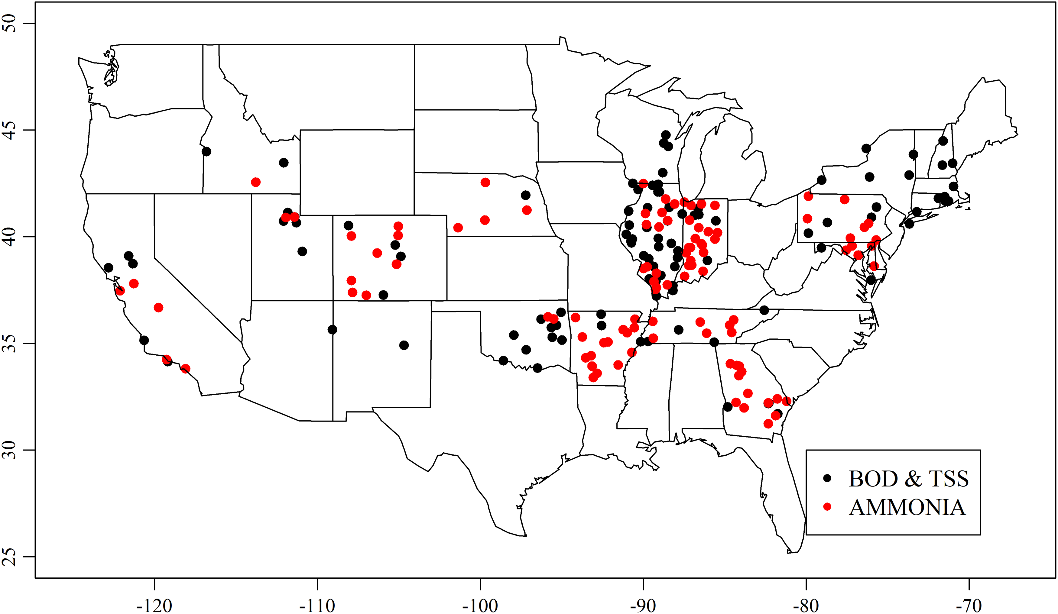
Location of randomly selected facilities with DMR data for BOD, TSS, and ammonia between 2004 and 2008. BOD, biochemical oxygen demand; DMR, discharge monthly report; TSS, total suspended solids.
DMR data are averages of samples taken over monitoring frequencies specified in individual facility permits. Like any laboratory and field data, DMR effluent values may have errors associated with sampling and analysis methods. However, data quality is controlled by most states that oversee the NPDES system and require plants to submit laboratory quality assurance/quality control (QA/QC) plans to comply with standards for accuracy and precision, based on standard methods for the examination of water and wastewater (www.standardmethods.org/; Oregon Department of Environmental Quality, 2009; APHA, AWWA, WEF, 2014).
GLM inputs include the natural log of the average monthly flow rate into the plant (A) and the capacity utilization (C), which is the reported monthly average flow rate divided by the design flow rate. In addition to A and C, the product AC was added as a covariate (Weirich et al., 2011). In the research by Weirich et al. (2011), these variables were used in a GLM to test the hypothesis that decentralization of wastewater infrastructure, necessarily associated with smaller treatment facilities, might have an impact on performance measured by compliance with permit discharge limits.
However, the residuals from this GLM were high in magnitude, auto-correlated and predictive ability of this model was limited. To improve on the model skill, we introduced two additional independent variables. The first variable, referred to as “lag”, which is the relative concentration of the pollutant in the previous month, was used by Weirich et al. to incorporate “persistence” or “inertia” in system performance and eliminate autocorrelation (Weirich et al., 2015). In addition to flow and historic compliance characteristics, we hypothesized that seasonality is a second variable that could account for a portion of compliance variability. Seasonal treatment operations can reflect temperature effects on biological transformation rates (Cornel and Weber, 2004). To capture seasonality effects, two cyclical covariates, sine (
Covariates and coefficients for the best GLM in the first Level of the hierarchical model for BOD and ammonia, as determined by BIC.
Results and Discussions
The results from the first and second levels of hierarchy for BOD are presented, followed by the results for ammonia. The best model and the results for TSS were similar to BOD, and in the interest of space, they are not shown. The best link function for the Gamma family and associated coefficients for the GLM are selected using the minimum BIC and are summarized in Table 1. The best models for BOD and ammonia are arrived at using the “stepAIC” function in the MASS package (Venables and Ripley, 2002) of R. In this BIC, values are computed for all combination of predictors, and the model with the least BIC value is selected as the best model. The candidate models and their corresponding BIC values, considered by this function, are provided in Supplementary Table S3.
BOD
The first level in the hierarchical model to predict relative BOD concentrations consists of the best GLM. Table 1 shows that A, C, the sine component, and lag appear in the best GLM, using the identity link function. The p values of the coefficients are significant at the 99% confidence level or higher. It should be noted that seasonality appears in this best GLM, indicating that there is a seasonal pattern of variation in the effluent relative BOD concentration. Lag also shows up in the best GLM, where the positive coefficient of the lag variable indicates that the relative BOD discharge in the previous month is predictive of relative BOD for the following month. This is in agreement with an earlier study that reported that the binomial variable associated with the occurrence of a violation was predictive of a violation in the subsequent month, and that especially for plants with lower capacity, discharge violations tend to persist often for several months (Weirich et al., 2015). Of all the variables in the best GLM, lag has the highest positive coefficient, indicating that the relative concentration in the previous month has the most significant effect in predicting the relative concentration in the current month.
The residuals from this model are close to zero at most locations, but at locations where the relative effluent BOD concentration is high, the best GLM is unable to capture these high values. It can be argued that once the effect of plant characteristics, seasonality, and lag is factored into the GLM, the residuals explain the small scale variability in the data. These local variations can be captured by the second level of hierarchy, Kriging. Figure 4 depicts the spatial map of the average value of residuals obtained from the best GLM using Kriging. It shows that the average magnitude of residuals across most of the country is close to zero, except for a region in Oklahoma and northeast Texas, which corresponds to a location where the relative BOD concentrations are higher than the rest of the country (0.5–1.4). Kriging (which fits a surface to the residuals as the function of latitude and longitude) can estimate only one value of residual at each location, for all months. The underlying assumption here is that the residuals are dependent only on the location and do not vary over time. The residuals obtained from GLM are not autocorrelated (figure not shown) and hence can be assumed to be independent and identically distributed. Averaging GLM residuals over time at every location allows a better fit of the variogram and consequently better Kriging estimates. So, in the second level of hierarchy, the average of the residuals from the best GLM for BOD is calculated at each location and a Kriging model is fit. Hierarchical model estimates are obtained by adding the average value of the predictions from the GLM to the predicted residual from the spatial model at each plant location. These estimates provide us with one predicted value for relative BOD at each location, based on annual average data for each plant.

Spatial map of average of residuals (at each location) obtained from GLM for relative BOD plotted using Kriging. GLM, Generalized Linear Model.
Ammonia
The best GLM for ammonia consists of the variables, A and lag, with the p values of the coefficients significant at 99% confidence level or higher. Once again, the positive coefficient for the lag variable indicates persistence of discharge levels from 1 month to another, including higher likelihood of successive violations. It is interesting to note that seasonality was not found to affect the relative ammonia concentration. This could result from the practice that ammonia is typically regulated by seasonal discharge limits, which tend to be higher in winter. Low temperatures particularly affect nitrification, and with uniformly low limits it might be expected to see a strong influence of the seasonal variable in the GLM. However, the leeway in ammonia discharge levels provided by seasonal permit limits may explain why this variable did not have a significant effect on compliance.
As for BOD, the average value of residuals from the best GLM for ammonia is spatially plotted using Kriging. Figure 5 shows the spatial patterns of the residuals. Once again, the magnitude of residuals is close to zero across the country, except for a small region in northeast Oklahoma. This is also the region with high relative ammonia concentration (0.5–1.8), indicating that the GLM is unable to capture high relative concentration values. These are the locations, where the second level of hierarchy explains the remainder of the variance. The predictions from Kriging are added to the average of the GLM predictions at each location, to get the hierarchical model predictions.

Spatial map of average of residuals (at each location) obtained from GLM for relative ammonia plotted using Kriging.
Model Validation
The predictive performance of the hierarchical model is evaluated in a drop 10% cross-validation mode. This is done by randomly dropping 10% of the plants in the BOD and ammonia data set and fitting a GLM and Kriging model on the remaining 90% plants. Hierarchical model estimates are obtained as the sum of the GLM and Kriging model predictions. The predictions are compared with the corresponding observations and the R2 value is computed. This is repeated 500 times to obtain 500 R2 values, which are shown as boxplots. Such a cross-validation approach stresses the model and provides estimate of the predictive capability. Unlike traditional approach, which uses a training and validation data set, the performance is beholden to these two data partitions. The drop 10% cross-validation approach has been used in water quality modeling (Zachman et al., 2007; Towler et al., 2009) and streamflow forecasting (Grantz et al., 2005; Regonda et al., 2006), among other applications.
In this process, we first decided to test the predictive performance of the first level of hierarchy, that is, the GLM due to the addition of seasonality and lag in addition to A, C, and AC. From the covariate set consisting of A, C, and AC, the best GLM is selected using the minimum BIC. For BOD, the independent variables in this model consisted of A and C, whereas for ammonia, the best model contained only variable A. Figure 6a shows the boxplot of R2 values from drop 10% cross-validation, when the best GLM was chosen from a predictor set consisting of A, C, and AC, and Fig. 6b shows the same using a predictor set of A, C, AC, seasonality, and lag. For Fig. 6a, the best model consisted of A and C, whereas for Fig. 6 (b), the best model consisted of A, C, sine component, and lag (for the first level of hierarchy in the model for BOD, refer to Table 1). Figure 7a and b shows the corresponding plots for ammonia. For Fig. 7a, the best model consisted of only A, whereas for Fig. 7b, the best model consisted of A and lag (for first level of hierarchy in the model for ammonia, refer to Table 1). It can be seen in these two figures that addition of seasonality and lag to the GLM covariates result in better predictive capability. In Fig. 6, we can see that addition of seasonality and lag to the GLM covariate set result in the increase of the median R2 value from about 0.02 to 0.5, whereas in Fig. 7, we can see it increases from about 0.05 to 0.3.
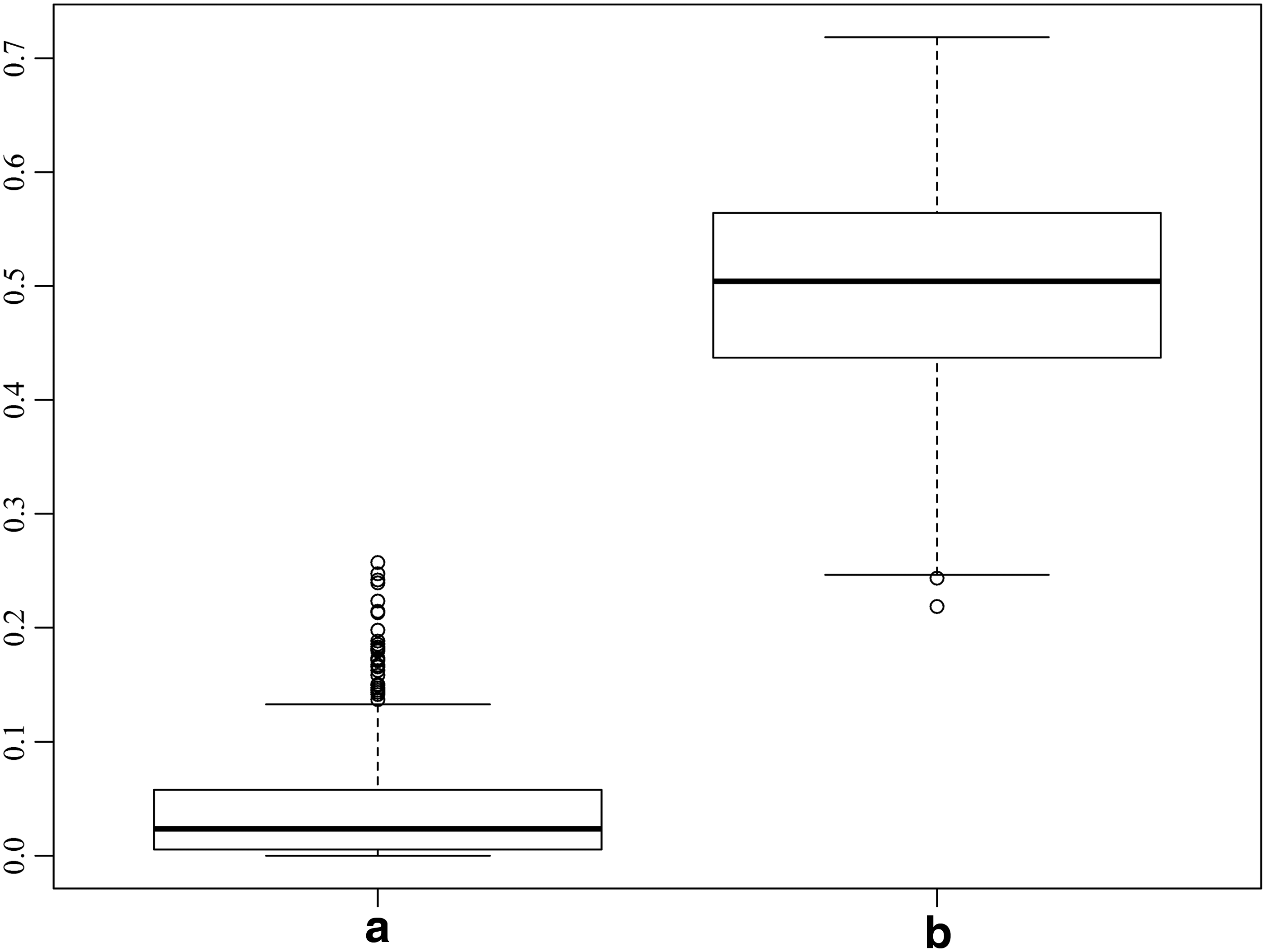
Boxplot of R2 values obtained by comparing observed and predicted relative BOD concentrations in the drop 10% cross-validation mode, when

Boxplot of R2 values obtained by comparing observed and predicted relative ammonia concentrations in the drop 10% cross-validation mode, when
Next we evaluate the improvement in predictive performance of the hierarchical model due to the addition of the second level of hierarchy: the spatial model, to the GLMs. From the spatial maps of the residuals, it is evident that this GLM captured most of the variability in the data except at locations where the relative concentrations were high (exceeding 0.5 for both BOD and ammonia). So, we evaluated the predictive performance of the GLM and the hierarchical model—GLM with Kriging model at these specific locations. Boxplots of R2 values are shown in Fig. 8a and b for BOD and in Fig. 9a and b for ammonia. For both BOD and ammonia, the two-level hierarchical model offers considerable improvement in the predictive performance over the first level of hierarchy, median R2 increases from 0.4 to 0.8 for BOD and from 0.3 to 0.75 for ammonia. Comparing the predictive performance of the hierarchical models for BOD and ammonia, it is apparent that the R2 values generally are slightly lower for ammonia than for BOD. This lower performance skill of the ammonia model could be due to either greater variability of ammonia removal itself or of permit limits, which vary both geographically and seasonally.
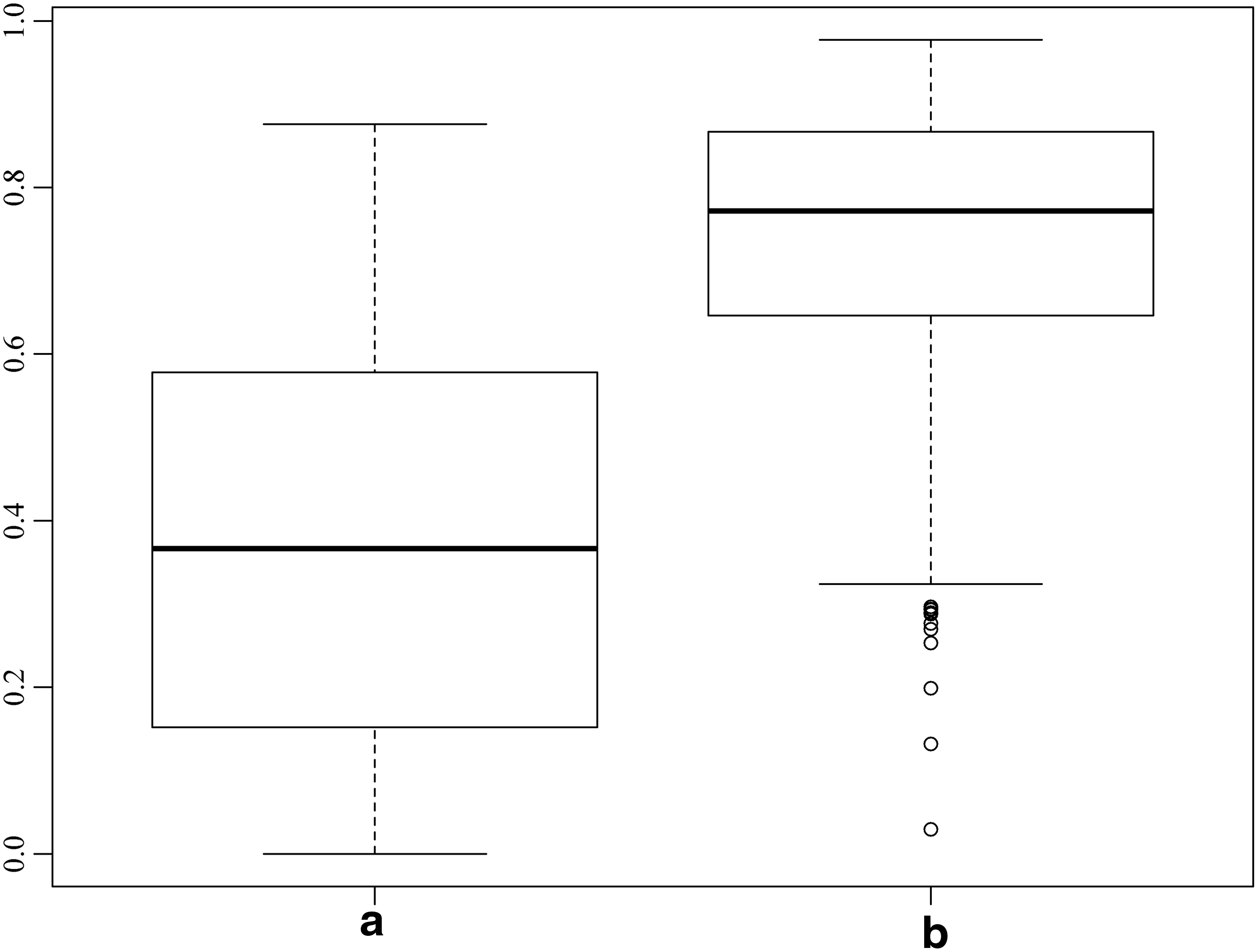
Boxplot of R2 values obtained by comparing observed and predicted relative BOD concentrations in the drop 10% cross-validation mode, at locations where relative BOD concentration exceeds 0.5 when

Boxplot of R2 values obtained by comparing observed and predicted relative ammonia concentrations in the drop 10% cross-validation mode, at locations where relative ammonia concentration exceeds 0.5 when
We observed that the spatial density of treatment plants in the sample was not uniform, even though the original sample from the ICIS database was randomly selected (Fig. 3), and, in fact, the geographic heterogeneity of the sample reflects the actual spatial density of facilities (number of plants/population) on a statewide basis, as reported by EPA (USEPA, 2008). To test the sensitivity of the hierarchical model to the spatial density of observations, the analysis was repeated for the region with the highest spatial density of observations (85°W to 95°W). It was found that the best GLM using the reduced BOD and ammonia data set had the same explanatory variables as the best GLM for the entire sample (figures not shown). In addition, the spatial map of the residuals for this smaller region shows similar patterns as the residuals map obtained using the entire data set, indicating that the hierarchical model is not sensitive to the spatial density of observations.
Conclusions
We report the results of a novel hierarchical modeling approach to capture the temporal and spatial variability of wastewater treatment compliance to permit limits for BOD, TSS, and ammonia. Data from more than 200 treatment plants for BOD and TSS and more than 100 plants for ammonia were used to build the hierarchical model, which enables diagnosis of treatment plants' compliance with existing discharge limits based on flow, hydraulic loading, seasonality, and prior performance. The advantage of this two-tiered hierarchical approach is that it individually models two different sets of factors, which affect compliance variables and act as major drivers of compliance variability along with local covariates, that is, latitude and longitude. In the first level of hierarchy, addition of seasonality and lag to the GLM consisting of A, C, and AC greatly enhances the predictive performance. For most regions across the country, where relative concentrations of pollutants are low (<0.5), the first level of hierarchy captures up to 70% of the variability in the data. Unlike earlier statistical models of wastewater treatment reliability (Niku and Schroeder, 1981; Oliveira and Sperling, 2008), process technology was not considered in the GLM. However, the result of our study, which up to 70% of the variability in BOD, TSS, and ammonia discharge levels relative to permit limits is accounted for by global operating characteristics (flow, capacity loading, and prior performance), and seasonality in the case of BOD and TSS, suggests that the influence of these variables, exerted over the facility lifetime, should be considered in wastewater treatment compliance evaluation.
For regions with higher relative pollutant concentrations, the GLM alone may not be enough. Addition of a spatial component helps account for some local variability in the data, providing further improvement in the predictive performance. The spatial maps of residuals can also act as a quick tool for regulatory agencies to identify regions of noncompliance, as the regions of high residuals correspond to the regions of high relative pollutant concentrations. Thus the hierarchical setup is more efficient in diagnosing and predicting noncompliance, especially for nutrients such as ammonia, which continue to be regulated on a local basis (Shapiro, 2012). Given that the geographical distribution of POTWs is not uniform with respect to population, this hierarchical framework also assuages concerns about the sensitivity of the model predictions to the spatial density of observations.
The hierarchical approach presented here can also be applied under other scenarios. The predictions from this hierarchical model can provide insight into how treatment plant compliance with nutrient limits might change if more stringent technology-based limits were imposed on a statewide, regional, or national scale. Furthermore, by incorporating other probability distributions in the first level of hierarchy, some other aspects of compliance may be modeled. For example, a binomial distribution in the first level of hierarchy can be used to model the probability of regulatory threshold exceedance; a Poisson distribution would enable hierarchical modeling of the number of permit violations expected at various locations across the country.
Footnotes
Acknowledgments
This research was part of the activities of the
Author Disclosure Statement
No competing financial interests exist.
References
Supplementary Material
Please find the following supplemental material available below.
For Open Access articles published under a Creative Commons License, all supplemental material carries the same license as the article it is associated with.
For non-Open Access articles published, all supplemental material carries a non-exclusive license, and permission requests for re-use of supplemental material or any part of supplemental material shall be sent directly to the copyright owner as specified in the copyright notice associated with the article.
