Impacts of Nonpoint Source Pollution on Water Quality in the Yuqiao Reservoir

Abstract

The Yuqiao Reservoir is an important drinking water source for the city of Tianjin. In recent years, the water quality of this reservoir has been seriously threatened by eutrophication resulting from increased nonpoint source pollution loads. In this study, we used a Soil and Water Assessment Tool (SWAT) model to calculate pollution loads (total nitrogen [TN] and total phosphorus [TP]) in the area surrounding the Yuqiao Reservoir. We then established a coupled two-dimensional hydrodynamic and water quality model that was used to simulate temporal and spatial distributions of TN and TP from June to September 2008. SWAT model results provided water quality boundary conditions for the coupled two-dimensional model. Results indicated that Liu Xiangying and Wu Baihu were the main TN inlets, and the average TN concentration in the reservoir was highest in September (3.74 mg/L). Meanwhile, the TP concentration in the eastern portion of the Yuqiao Reservoir was higher than that in the west, and the average TP concentration peaked in August (1.56 mg/L). The combination of the SWAT model and two-dimensional hydrodynamic and water quality model provides an effective method to simulate water pollution with consideration of various factors.

Introduction

Storage capacities of most lakes and reservoirs in China are shrinking. Moreover, the water quality is worsening and eutrophication is becoming a serious issue (Shen et al., 2012b). A growing number of studies have shown that nonpoint source pollution is an important factor in eutrophication problems (Ongley et al., 2010; Lai et al., 2011; Li et al., 2011). Using the export coefficient model, Ma et al. (2011) assessed the influence of nonpoint source pollution loadings (total nitrogen [TN] and total phosphorus [TP]) in the Three Gorges Reservoir (TGR) area. Chen et al. (2013) estimated the spatial and temporal distributions of nonpoint source pollutants in a drinking water reservoir that supplies the city of Ningbo, China. Meanwhile, Liu et al. (2013) developed an interval-fuzzy, two-stage stochastic nonpoint source pollution mitigation (IFTNS) model that they used to analyze a nutrient discharge trading program in the Lake Tai River basin. All of these studies showed that water quality in reservoirs in China is deteriorating.

Water quality of the Yuqiao Reservoir has recently worsened due to changes in the upstream water environment (Liu et al., 2008; Chen et al., 2012; Li et al., 2015). In addition, the impact of nonpoint source pollution on the water quality in source regions for drinking water has become increasingly apparent (He et al., 2015), especially during flood seasons (Owens et al., 2008; Liu et al., 2014). When it rains, surface pollutants are likely to be leached, distributed, and transported by surface runoff, leading to sharp increases in pollution loads and considerable pollutant transport to reservoir areas. Some studies indicated that nonpoint source pollution carried by surface runoff has become one of the most significant sources of pollution during rainy seasons (Zhang et al., 2011; Shen et al., 2012a).

This study investigated the impacts of nonpoint source pollution (TN and TP) on water quality in the Yuqiao Reservoir during flood seasons. A coupled two-dimensional hydrodynamic and water quality model was developed to simulate the temporal and spatial distributions of TN and TP within the Yuqiao Reservoir from June to September in 2008. Owing to a lack of water quality data from inlets in the area surrounding the Yuqiao Reservoir, monthly pollution loads and a TN and TP concentration time series for each inlet were generated based on results calculated with the Soil and Water Assessment Tool (SWAT) model, which was used to analyze TN and TP inflows around the Yuqiao Reservoir. The combination of the SWAT model and two-dimensional hydrodynamic and water quality model provides an effective method for analyzing the distribution of nonpoint source pollution when adequate data are not available, and provides significant reference information that can help guarantee the safety of downstream water supplies.

Study Area

The Yuqiao Reservoir is located 4 km east of Jixian, Tianjin between longitude 117°25′E and latitude 40°02′N. The reservoir drainage area is 2.06 × 10³ km² and the reservoir can store a total water volume of 1.56 × 10⁹ m³ (Liu et al., 2008). Upstream inflows to the reservoir include the Lin River, Sha River, and Li River (Fig. 1a). The average annual runoff is 5.06 × 10⁸ m³.

FIG. 1.

Study area location. (a) Yuqiao Reservoir River basin and its location in the Haihe River basin. (b) Map of the Water Diversion Project from the Luan He River to Tianjin City. (c) Yuqiao Reservoir inlets and outlets.

Since the construction of the Water Diversion Project from the Luan He River to Tianjin City in 1983 (Fig. 1b), the Yuqiao Reservoir has become the most important water source for Tianjin. Although flood control and water supply are the main functions of the Yuqiao Reservoir, it also contributes to agricultural irrigation and electric power generation. The Panjiakou Reservoir is located downstream of the Luan He River, and is the water source for the Yuqiao Reservoir. The water diverted from the Luan He River flows into the Daheiting Reservoir before making its way into the Li River. As the Sha River and Li River converge into the Guo River, the water diverted from the Luan He River finally flows into the Yuqiao Reservoir through the Guo River inlet (Fig. 1c).

The Yuqiao Reservoir River basin includes 11 rivers longer than 20 km and more than 30 rivers shorter than 20 km. Those branches converge into three rivers: the Lin River, Sha River, and Li River. These three rivers transport nonpoint source pollution from sources such as livestock and poultry feces, as well as fertilizers and point source pollution from water diversion and upstream plants. However, in the early 2000s the Chinese government undertook measures to control point source pollution, and the plants that seriously affected water quality in the study area were closed. Given that the plants were closed before the study period, pollution from upstream plants was excluded from the SWAT model used in this study. Apart from water diverted from the Luan He River (point source pollution), the water quality in the Yuqiao Reservoir was mainly affected by nonpoint source pollution. Due to the economic development and population explosion in China, in recent years, increasing levels of pollutants have been discharged into upstream rivers or the surrounding area that in turn worsen the Yuqiao Reservoir water quality.

Methods and Models

SWAT model

Description of the SWAT model

The SWAT model is a distributed-parameter model that was developed by the United States Department of Agriculture (USDA) in the early 1990s (Lee et al., 2010). In this study, the SWAT model was used to simulate TN and TP loads around the Yuqiao Reservoir. The SWAT model has been used worldwide to simulate the impacts of land management measures on agricultural nonpoint source pollution (Baker and Miller, 2013; Wellen et al., 2014; Abbaspour et al., 2015). Scientists in China carried out studies based on the SWAT model in the Lake Tai River basin, the East River basin, Miyun Reservoir, and the TGR (Wu and Chen, 2013; Zhang et al., 2013; Shen et al., 2014; Zhu et al., 2015) with satisfactory simulation results, thus verifying the applicability of the SWAT in China.

In this study, the Yuqiao Reservoir River basin was divided into 40 subcatchments and 359 hydrological response units based on Digital Elevation Models (DEMs), land use/land cover, and soil type images (Fig. 2a). DEM images were obtained from the Advanced Spaceborne Thermal Emission and Reflection Radiometer Global Digital Elevation Model (ASTER GDEM) dataset compiled in 2009 with a resolution of 30 m. Land use and land cover images (250 m) taken in 2006 were provided by the Institute of Remote Sensing and Digital Earth, Chinese Academy of Sciences. Land use data (Fig. 2b), soil data (Fig. 2c), and slopes (Fig. 2d) in the study area were also defined. Soil type images and soil data were from the Institute of Soil Science and rendered at a scale of 1:1,000,000.

FIG. 2.

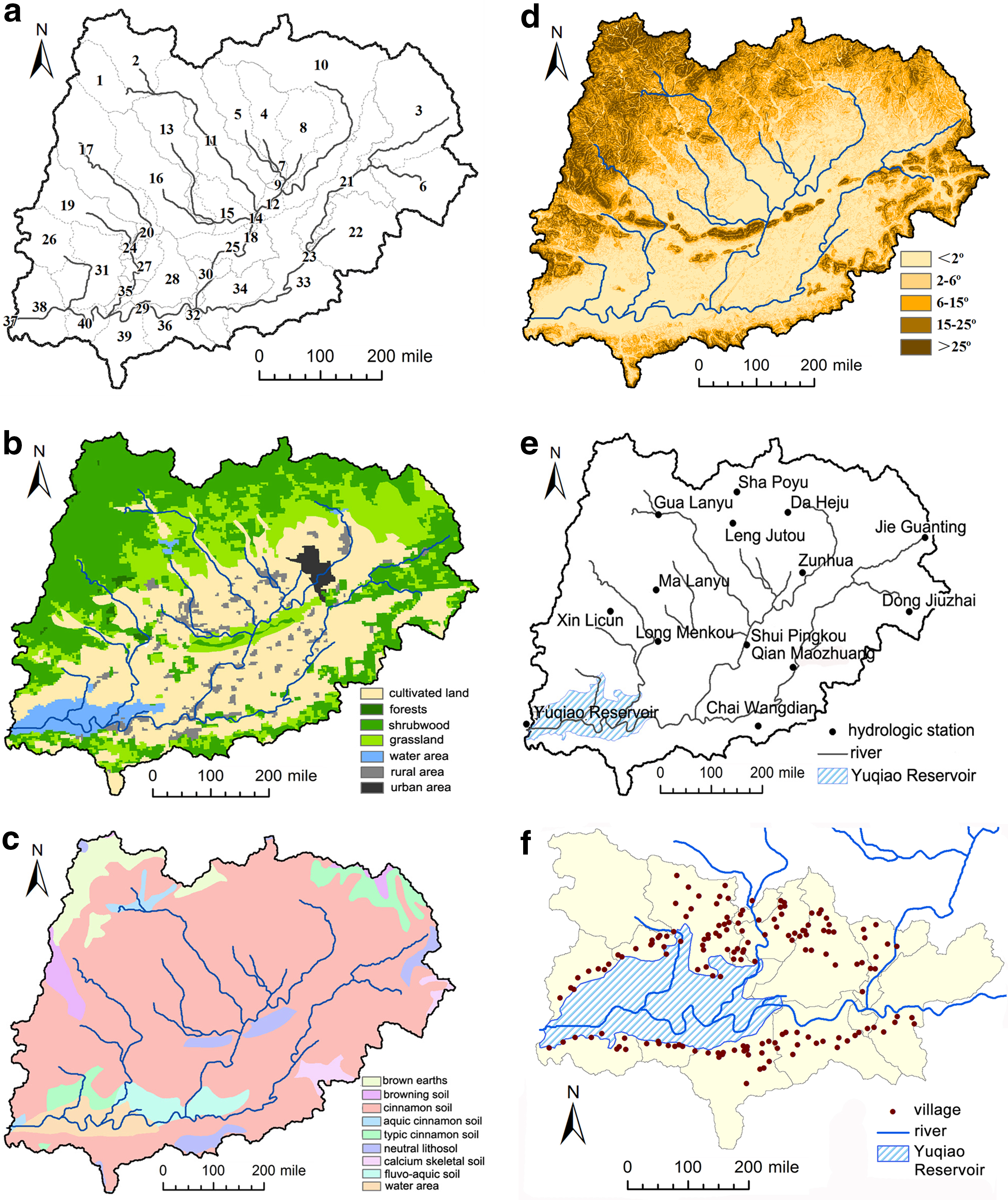
Basic information used in the SWAT model. (a) Forty subcatchments in the study area. (b) Land use in the study area. (c) Soil types in the study area. (d) Slopes in the study area. (e) Distribution of hydrologic stations in the study area. (f) Villages around the Yuqiao Reservoir area. SWAT, Soil and Water Assessment Tool.

Meteorology and pollution data were also input into the model (Fig. 2e). Precipitation and runoff data were extracted from the China Hydrological Year Book. Meteorological data, including temperature, wind speed, relative humidity, and sunshine duration were from the China Meteorological Data Sharing Service System.

Statistics for villages and towns near the Yuqiao Reservoir were from “The survey of Yuqiao Reservoir in 2008” and “The official report on water resources of Tianjin in 2008.” According to the survey data for 160 villages around the Yuqiao Reservoir (Fig. 2f), the amount of domestic sewage in each subcatchment can be estimated as follows: \documentclass{aastex}\usepackage{amsbsy}\usepackage{amsfonts}\usepackage{amssymb}\usepackage{bm}\usepackage{mathrsfs}\usepackage{pifont}\usepackage{stmaryrd}\usepackage{textcomp}\usepackage{portland, xspace}\usepackage{amsmath, amsxtra}\pagestyle{empty}\DeclareMathSizes{10}{9}{7}{6}\begin{document} \begin{align*} A = Q \times p \times n \prime / n \times d , \tag{1} \end{align*} \end{document}

where A is the amount of daily domestic sewage in each subcatchment, Q is the amount of total waste water, p is the percentage of domestic sewage in the amount of waste water, n is the population involved in the survey, d is the days of the survey, and n′ is the population in the subcatchment. The amount of domestic sewage discharge to rivers is estimated as follows: \documentclass{aastex}\usepackage{amsbsy}\usepackage{amsfonts}\usepackage{amssymb}\usepackage{bm}\usepackage{mathrsfs}\usepackage{pifont}\usepackage{stmaryrd}\usepackage{textcomp}\usepackage{portland, xspace}\usepackage{amsmath, amsxtra}\pagestyle{empty}\DeclareMathSizes{10}{9}{7}{6}\begin{document} \begin{align*} D = Q \times i , \tag{2} \end{align*} \end{document}

where D is the amount of domestic sewage discharged to rivers, Q is the amount of domestic sewage in each subcatchment, and i is the domestic sewage discharge rate in the rural area. According to “The survey of Yuqiao Reservoir in 2008” and relevant surveys of the Haihe River basin (Zhu, 2011), i is equivalent to 0.42.

Based on Equations (1) and (2), and according to the village statistics, the amount of domestic sewage discharged to the rivers in each subcatchment was estimated and then added as point source pollution to a simulated drainage outlet in each subcatchment. In this way, the nonpoint source pollution loads resulting from the domestic sewage of villages in each subcatchment were obtained in the SWAT model.

Surveys of villages around the Yuqiao Reservoir were used to determine the annual amounts of residential and livestock feces in the surrounding subcatchments (Table 1). After eliminating some of the feces that were used for organic fertilizer, the remainder was added to each subcatchment on a daily basis to simulate the daily accumulation of feces.

Table 1.

Annual Amount (in Tons, t) of Residential and Livestock Feces in Subcatchments Surrounding the Yuqiao Reservoir

	Feces source
Subcatchment number	Chickens (t)	Ducks (t)	Pigs (t)	Sheep (t)	Cows (t)	Residents (t)
24	372.7	2,800.8	497.1	852.0	230.5	4,881.6
27	4,572.1	439.7	713.6	300.9	892.2	3,000.7
28	324.4	21.2	0.0	115.9	2,965.5	2,378.9
30	112.0	0.0	3,555.9	232.1	3,689.7	3,479.5
31	1,288.6	366.5	6,700.6	293.3	1,661.0	2,455.0
34	64.2	0.0	0.0	26.1	193.4	949.1
35	203.2	0.0	2,688.4	396.4	0.0	2,207.3
36	509.5	64.1	5,420.2	417.3	10,555.6	6,254.9
38	2,492.0	100.3	998.0	216.7	334.4	3,003.6
39	1,252.0	62.0	21,645.3	23.8	107.5	2,852.9

The SWAT model allows land management practices to be simulated. In the study area, the crop-planting pattern rotates winter wheat and summer maize, so these scheduled management operations were added to farmlands (Table 2).

Table 2.

Land Management Operations in Study Area in 2008

Date	Operations	Details
February 20	Tillage operation	Surface tillage (5 cm)
March 5	Fertilizer application	Organic fertilizer application (1,822.5 kg/ha)
March 10	Irrigation	to 60 mm depth
April 20	Fertilizer application	KH₂PO₄ applied at 0.3 kg/ha
May 1	Irrigation	to 60 mm depth
June 10	Harvest operation	Winter wheat harvest
June 13	Fertilizer application	Organic fertilizer applied at 2,082.9 kg/ha
June 15	Plant operation	Summer maize planting
June 16	Irrigation	to 60 mm depth
July 25	Fertilizer application	Urea applied at 177 kg/ha
July 27	Tillage operation	Intertillage (15 cm)
August 20	Fertilizer application	Urea applied at 262.5 kg/ha
August 21	Tillage operation	Intertillage (15 cm)
August 22	Irrigation	to 60 mm depth
August 23	Fertilizer application	Urea applied at 75 kg/ha
August 31	Irrigation	to 15 mm depth
September 5	Tillage operation	Surface tillage (5 cm)
September 30	Harvest operation	Summer maize harvest
October 5	Fertilizer application	Organic fertilizer applied at 1,822.5 kg/ha
October 7	Tillage operation	Deep tillage (35 cm)
October 8	Irrigation	to 60 mm depth
October 10	Plant operation	Winter wheat planting
October 12	Tillage operation	Surface tillage (0.5 cm)
November 25	Irrigation	to 60 mm depth
November 26	Tillage operation	Surface tillage (5 cm)

The water diversion periods in 2008 were from April 13 to May 30, August 27 to September 11, and October 27 to November 29. According to data gathered for the Daheiting Reservoir, a water inlet was added to the initial point of the river in subcatchment 3, where the flow (Fig. 3) and water quality data (Fig. 4) during water diversion periods were input as point source pollution.

FIG. 3.

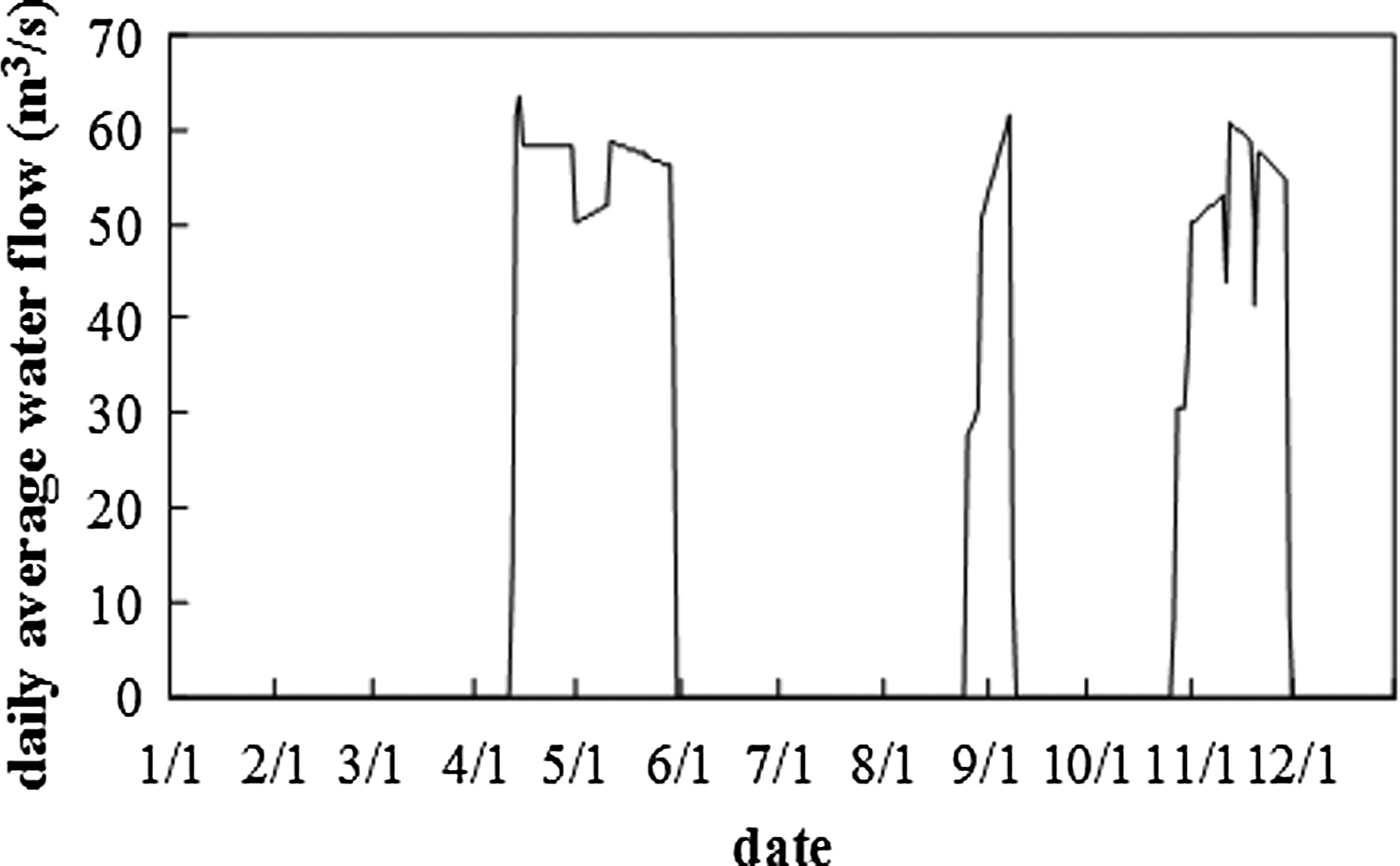
Daily average water flow from the Daheiting Reservoir outlet during 2008.

FIG. 4.

The monthly water quality data for the Daheiting Reservoir during 2008. (a) TN concentration. (b) TP concentration. TN, total nitrogen; TP, total phosphorus.

Calibration and validation of the SWAT model

The Sha River is the main source of flow and pollution loads in the Yuqiao Reservoir River basin. Therefore, we used water quality data from the Shui Pingkou hydrologic station (Fig. 2e), which is located in the middle reach of the Sha River (longitude 117°51′E and latitude 40°06′N), to calibrate and validate the SWAT model.

The SWAT model calibration was carried out by autocalibration performed using the Generalized Likelihood Uncertainty Estimation (GLUE) procedure available in the SWAT Calibration and Uncertainty Procedures (SWAT-CUP) (Abbaspour et al., 2007). Hydrologic parameters were calibrated before water quality parameters and their feasibility were identified. Before the calibration, sensitive model parameters were identified by performing a sensitivity analysis using SWAT-CUP. Since additional iterations in the calibration produced more possible optimal parameters, the number of iterations used in this study was limited to 5,000. Calibration results for hydrologic and water quality parameters are shown in Tables 3 and 4.

Table 3.

Calibrated Hydrologic Parameters Used in Soil and Water Assessment Tool Model with Their Ranges and Calibrated Values

				Range
Parameter	Description	Module	Assignment method	Lower limit	Upper limit	Calibrated value
SURLAG	Surface runoff lag time	.bsn	Given value	1	24	16.24
EVRCH	Reach evaporation adjustment factor	.bsn	Given value	0.5	1	0.89
GW_DELAY	Groundwater delay	.gw	Given value	0	500	16.79
ALPHA_BF	Baseflow alpha factor	.gw	Given value	0	1	0.15
GWQMN	Threshold depth of water in the shallow aquifer required for the return flow to occur	.gw	Given value	0	5000	841.88
GW_REVAP	Groundwater revaporization coefficient	.gw	Given value	0.02	0.2	0.17
REVAPMN	Threshold depth of water in the shallow aquifer required for revaporization to occur	.gw	Given value	0	500	167.38
RCHRG_DP	Deep aquifer percolation fraction	.gw	Given value	0	1	0.76
GW_SPYLD	Specific yield of the shallow aquifer	.gw	Given value	0	0.4	0.24
ESCO	Soil evaporation compensation factor	.hru	Given value	0.01	1	0.39
EPCO	Plant uptake compensation factor	.hru	Given value	0.01	1	0.83
OV_N	Manning's “n” value for overland flow	.hru	Multiplicative value	−0.25	0.25	−0.10
CN2	Initial SCS Runoff curve number for moisture condition II	.mgt	Multiplicative value	−0.25	0.25	−0.24
CH_N2	Manning's “n” value for the main channel	.rte	Given value	0	0.3	0.25
CH_K2	Effective hydraulic conductivity in the main channel alluvium	.rte	Given value	0	150	9.34
ALPHA_BNK	Baseflow alpha factor for bank storage	.rte	Given value	0	1	0.01
CH_K1	Effective hydraulic conductivity in the tributary channel alluvium	.sub	Given value	5	150	10.21
CH_N1	Manning's “n” value for the tributary channels	.sub	Given value	0.01	0.3	0.06
SOL_K	Saturated hydraulic conductivity	.sol	Given value	3.15–51.10 (changing according to soil types)
SOL_Z	Depth from soil surface to bottom of layer	.sol	Given value	100–1120 (changing according to soil types)
SOL_AWC	Available water capacity of the soil layer	.sol	Given value	0.05–0.13 (changing according to soil types)
SOL_ALB	Moist soil albedo	.sol	Given value	0.01–0.17 (changing according to soil types)
USLE_K	USLE equation soil erodability (K) factor	.sol	Given value	0.24–0.38 (changing according to soil types)
RES_SED	Initial sediment concentration in the reservoir	.res	Given value	1.5
RES_NSED	Equilibrium sediment concentration in the reservoir	.res	Given value	1.5

Table 4.

Calibrated Water Quality Parameters of Soil and Water Assessment Tool Model with Ranges and Calibrated Values

				Range
Parameter	Description	Module	Assignment method	Lower limit	Upper limit	Calibrated value
CMN	Rate factor for humus mineralization of active organic nutrients	.bsn	Given value	0.001	0.003	0.002
NPERCO	Nitrogen percolation coefficient	.bsn	Given value	0.01	1	0.0101
PPERCO	Phosphorus percolation coefficient	.bsn	Given value	10	17.5	13.12
PHOSKD	Phosphorus soil partitioning coefficient	.bsn	Given value	100	200	160.30
PSP	Phosphorus sorption coefficient	.bsn	Given value	0.01	0.7	0.60
RSDCO	Residue decomposition coefficient	.bsn	Given value	0.02	0.1	0.08
RS2	Benthic source rate for dissolved phosphorus in the reach at 20°C	.swq	Given value	0.001	0.1	0.01
RS3	Benthic source rate for NH₄-N in the reach at 20°C	.swq	Given value	0	1	0.16
RS4	Rate coefficient for organic N setting in the reach at 20°C	.swq	Given value	0.001	0.1	0.015
RS5	Organic phosphorus setting rate in the reach at 20°C	.swq	Given value	0.001	0.1	0.037
RK2	Oxygen reaeration rate in accordance with Fickian diffusion in the reach at 20°C	.swq	Given value	0	100	50.76
RK4	Benthic oxygen demand rate in the reach at 20°C	.swq	Given value	0	100	91.05
BC1	Rate constant for biological oxidation of NH₄ to NO₂ in the reach at 20°C	.swq	Given value	0.1	1	0.14
BC2	Rate constant for biological oxidation of NO₂ to NO₃ in the reach at 20°C	.swq	Given value	0.2	2	0.21
BC3	Rate constant for hydrolysis of organic N to NH₄ in the reach at 20°C	.swq	Given value	0.2	0.4	0.25
BC4	Rate constant for mineralization of organic P to dissolved P in the reach at 20°C	.swq	Given value	0.01	0.7	0.38
SOL_SOLP	Initial soluble P concentration in the soil layer	.chm	Given value	1.00–35.00 (changing according to soil types)
SOL_ORGN	Initial organic N concentration in the soil layer	.chm	Given value	99.43–1648.86 (changing according to soil types)
SOL_ORGP	Initial organic P concentration in the soil layer	.chm	Given value	25.89–523.04 (changing according to soil types)
SOL_NO3	Initial NO₃ concentration in the soil layer	.chm	Given value	2.28–6.33 (varies according to soil type)
RES_ORGP	Initial organic P concentration in the reservoir	.res	Given value	0.01
RES_SOLP	Initial soluble P concentration in the reservoir	.res	Given value	0.02
RES_ORGN	Initial organic N concentration in the reservoir	.res	Given value	0.48
RES_NO3	Initial NO3 concentration in the reservoir	.res	Given value	1.00

There are two types of parameters in the SWAT model. One is that the initial values of the parameters are identical for all subcatchments such that the existing parameter value is replaced by a given value during autocalibration. Another parameter is that the initial values of the parameters vary among subcatchments. An approach to estimate distributed parameters is by calibrating a modification term, which means the existing parameter value is multiplied by 1 + x, where x is a given value that ranges from −0.25 to +0.25. In this study, OV_N and CN2 are distributed parameters. Therefore, “−0.1” and “−0.24” were not the actual calibrated values, but instead part of the multipliers: (1 – 0.1) and (1 – 0.24).

The relative error Re, the correlation coefficient R², and the Nash–Sutcliffe coefficient E_ns were used to evaluate the model adaptability. The formula for E_ns is as follows: \documentclass{aastex}\usepackage{amsbsy}\usepackage{amsfonts}\usepackage{amssymb}\usepackage{bm}\usepackage{mathrsfs}\usepackage{pifont}\usepackage{stmaryrd}\usepackage{textcomp}\usepackage{portland, xspace}\usepackage{amsmath, amsxtra}\pagestyle{empty}\DeclareMathSizes{10}{9}{7}{6}\begin{document} \begin{align*} { E_ { ns } } = 1 - { \frac { \mathop \sum \limits_ { i = 1 } ^n { { { \left( { { Q_ { { o_i } } } - { Q_ { { s_i } } } } \right) } ^2 } } } { \mathop \sum \limits_ { i = 1 } ^n { { { \left( { { Q_ { { o_i } } } - { Q_ { avg } } } \right) } ^2 } } } } , \tag { 3 } \end{align*} \end{document}

where Q_o is the observed value, Q_p is the simulated value, Q_avg is the average observed value, and n is the number of observed values. The closer E_ns is to one, the more reliable the model.

Due to missing measurements, the water quality data were incomplete. Therefore, the lengths of the observed data series periods for the TN and TP concentrations differed. There was a substantial amount of data available for TN between July 2006 and December 2008, while extensive data for TP was available for the period between January 2006 and June 2008. Therefore, periods with relatively complete data were selected for use as calibration and validation periods.

Variations in observed and simulated TN concentrations were generally consistent (Fig. 5). During the calibration period, Re was −6.52%, R² was 0.61, and E_ns was 0.50. These values in the validation period were −0.05%, 0.54, and 0.53, respectively (Table 5).

FIG. 5.

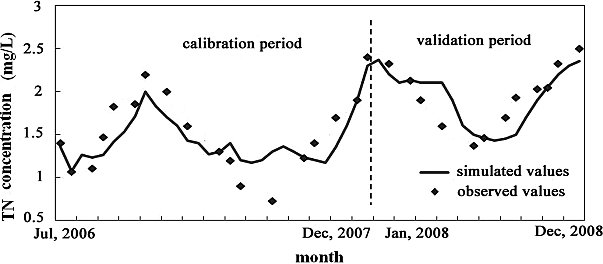
The simulated and observed TN concentrations.

Table 5.

Comparison Between Simulated and Observed Total Nitrogen Values

	Monthly average value (mg/L)
	Observed value	Simulated value	Re%	R²	E_ns
Calibration period	1.473	1.377	−6.52	0.61	0.50
Validation period	1.935	1.934	−0.05	0.54	0.53

The variations in observed and simulated TP values were generally consistent (Fig. 6). During the calibration period, Re was −6.55%, R² was 0.58, and E_ns was 0.56. During the validation period these values were 3.11%, 0.53, and 0.51, respectively (Table 6).

FIG. 6.

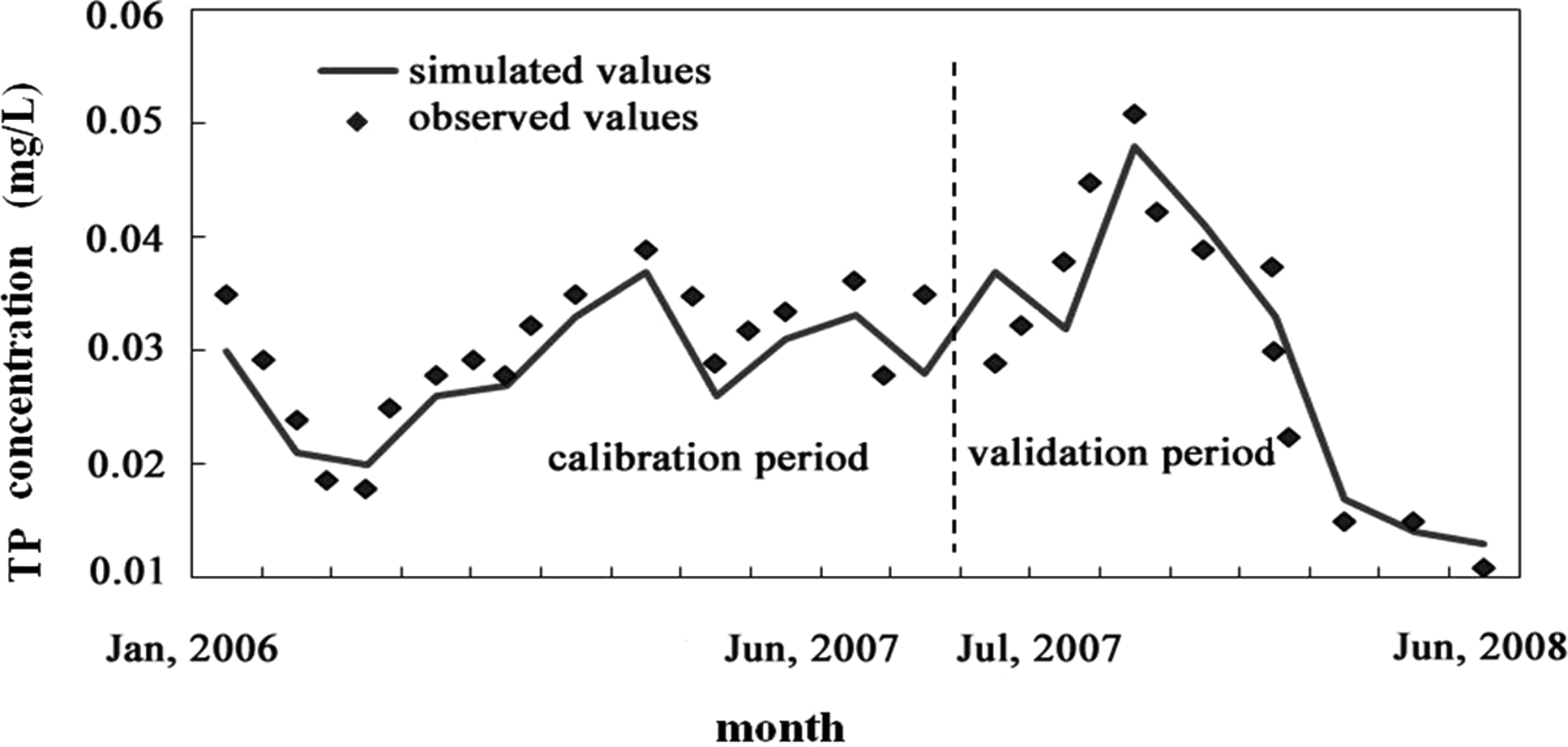
Simulated and observed TP concentrations.

Table 6.

Comparison Between Simulated and Observed Total Phosphorus Values

	Monthly average value (mg/L)
	Observed value	Simulated value	Re%	R²	E_ns
Calibration period	0.031	0.029	−6.55	0.58	0.56
Validation period	0.027	0.028	3.11	0.53	0.51

Analysis of pollution sources (TN and TP)

In the analysis of pollution loads derived from different sources, contrasting experiments were applied. First, all pollution sources were added into the SWAT model, and the simulated results in 2008 were regarded as the control group. Then, the simulation was run again with each pollution source removed, and the simulated results were regarded as experimental groups. By comparison with the control group, the pollution load resulting from each source could then be estimated. Likewise, for the total pollution load, the experimental group results were obtained with all pollution sources removed, such that comparisons with the control group allowed the pollution load resulting from all sources to be estimated.

According to the simulation results of the SWAT model in 2008 (Table 7), the average annual TN inflow reached 2,014.6 tons, of which the upstream water diversion accounted for the largest portion (43.4%). Other sources, including the middle and upper reaches, as well as forests and grasslands around the Yuqiao Reservoir, accounted for 33.9% of the total amount of TN with an inflow of 682.1 tons. Wastewater from restaurants contributed 173.1 tons of TN, and comprised 8.6% of the total. The proportions arising from farmlands (136.5 tons), domestic sewage (94.5 tons), and animal and resident feces (54.7 tons) were 6.8%, 4.7%, and 2.7%, respectively, of the total. Apart from upstream water diversion (point-source pollution), the main TN source in the Yuqiao Reservoir was nonpoint source pollution (56.6% in total), which significantly influenced the water quality in the Yuqiao Reservoir during nondiversion periods (Table 7).

Table 7.

Proportions of Total Nitrogen and Total Phosphorus Loads in 2008

Pollutant sources	TN (t)	Proportion (%)	TP (t)	Proportion (%)
Upstream water diversion	873.8	43.4	26.7	17.5
Farmlands	136.5	6.8	13.3	8.7
Resident and livestock feces	54.7	2.7	40.6	26.6
Wastewater from restaurants	173.1	8.6	22.3	14.6
Domestic sewage	94.5	4.7	12.3	8.1
Other sources	682.1	33.9	38.0	24.6

TN, total nitrogen; TP, total phosphorus.

The average annual TP inflow is 152.8 tons, with resident and livestock feces (40.6 tons) and other sources (38.0 tons) contributing the largest proportion (26.6% and 24.6%, respectively) of the total. Upstream water diversion (26.7 tons) and wastewater from restaurants (22.3 tons) accounted for 17.5% and 14.6% of all TP sources. Meanwhile, farmlands (13.3 tons) and domestic sewage (12.3 tons) accounted for 8.7% and 8.1%, respectively, of the total. In general, nonpoint TP pollutant sources were variable and thus required comprehensive treatment.

In terms of seasonal TN proportions, upstream water diversion was the dominant TN source in spring (from March to May) and autumn (from September to November), representing 66.7% and 61.3% of the total, respectively (Fig. 7). In summer (from June to August) and winter (from December to February), TN was mainly from other sources that contributed 25.3% and 72.5%, respectively, to the total (Fig. 7).

FIG. 7.

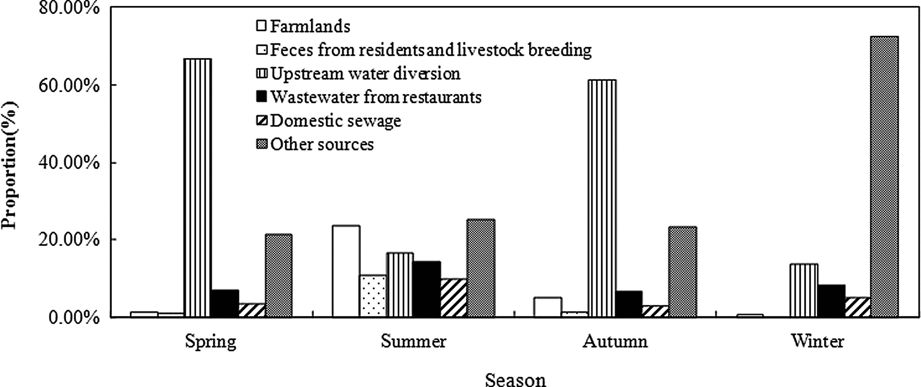
Seasonal proportions of TN sources in 2008.

In spring and autumn, upstream water diversion, at 34.6% and 53.4%, was the leading source of TP pollutants (Fig. 8). However, feces and wastewater from restaurants were the main contributors to TP pollutants in the summer and winter (40.4% and 32.5%, respectively; Fig. 8).

FIG. 8.

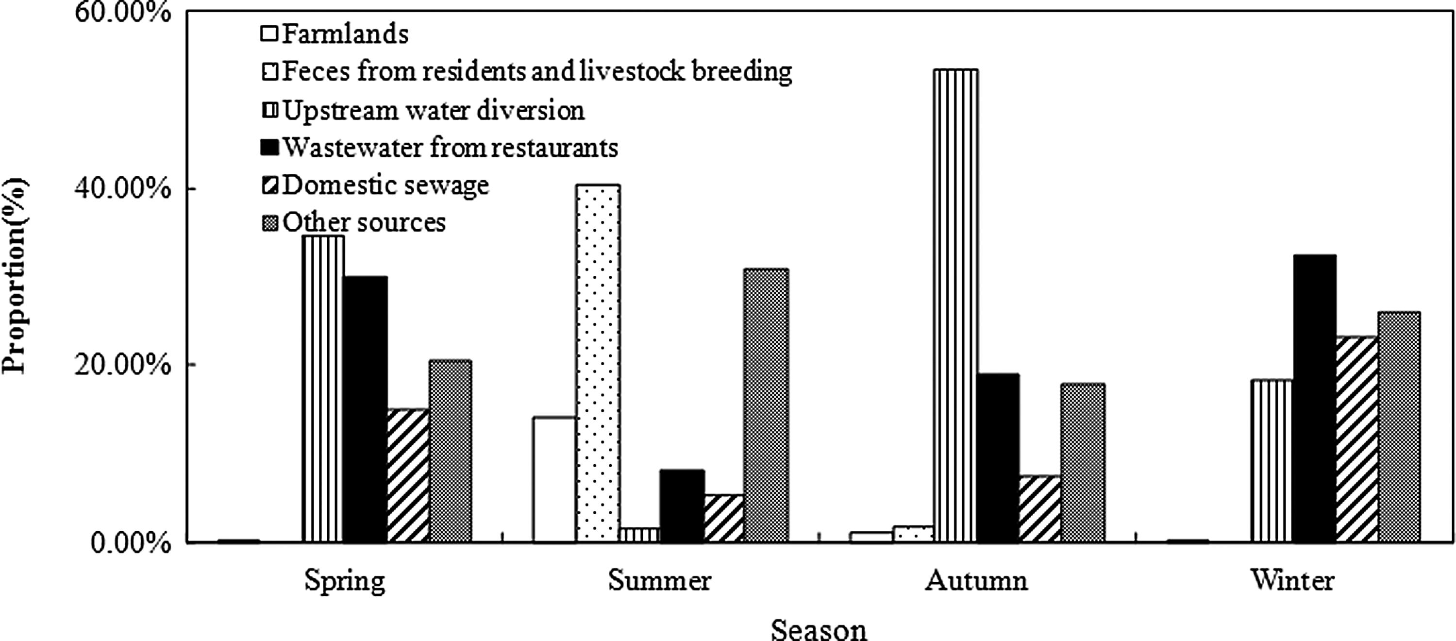
Seasonal proportions of TP sources in 2008.

This trend is consistent with the 2008 water diversion periods: April 13 to May 30, August 27 to September 11, and October 27 to November 29. Water was diverted from the Luan He River in the spring and autumn, and during this time upstream water diversion was the main TN and TP source.

Results for the SWAT model were calculated on a daily time scale. The monthly TN and TP pollution loads were obtained by summing the calculated results for daily TN and TP pollution loads (Fig. 9). The TN pollution loads were high in May (over 300 tons) and November (almost 500 tons) because of the large amount of upstream water diverted during these 2 months (Fig. 3). For TP, the pollution loads peaked at ∼30 tons in August. Moreover, the values during the flood season (June to September) accounted for most of the total TP during the year, suggesting that the pollution loads of TP were mainly caused by nonpoint source pollution associated with storm runoff during the rainy season.

FIG. 9.

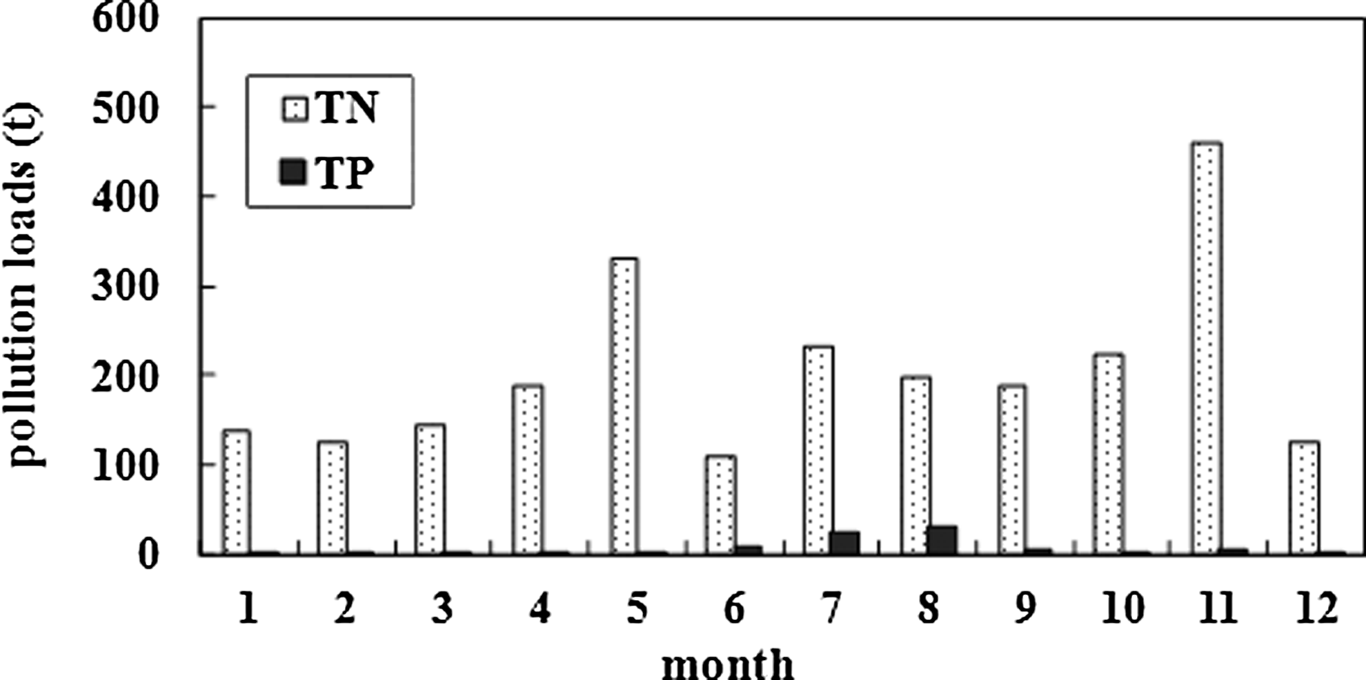
Monthly TN and TP pollution loads in 2008.

Coupled two-dimensional hydrodynamic and water quality model

Methods of the coupled two-dimensional model

Governing equations

The hydrodynamic model is based on the Reynolds-averaged and incompressible Navier–Stokes equations and subject to Boussinesq and hydrostatic pressure assumptions.

The two-dimensional unsteady shallow water equations are given below (Heniche et al., 2000). The equation of continuity is as follows: \documentclass{aastex}\usepackage{amsbsy}\usepackage{amsfonts}\usepackage{amssymb}\usepackage{bm}\usepackage{mathrsfs}\usepackage{pifont}\usepackage{stmaryrd}\usepackage{textcomp}\usepackage{portland, xspace}\usepackage{amsmath, amsxtra}\pagestyle{empty}\DeclareMathSizes{10}{9}{7}{6}\begin{document} \begin{align*} { \frac { \partial h } { \partial t } } + { \frac { \partial \left( { hu } \right) } { \partial x } } + { \frac { \partial \left( { hv } \right) } { \partial y } } = 0. \tag { 4 } \end{align*} \end{document}

The momentum conservation equations are as follows: \documentclass{aastex}\usepackage{amsbsy}\usepackage{amsfonts}\usepackage{amssymb}\usepackage{bm}\usepackage{mathrsfs}\usepackage{pifont}\usepackage{stmaryrd}\usepackage{textcomp}\usepackage{portland, xspace}\usepackage{amsmath, amsxtra}\pagestyle{empty}\DeclareMathSizes{10}{9}{7}{6}\begin{document} \begin{align*} { \frac { \partial \left( { hu } \right) } { \partial t } } + { \frac { \partial \left( { h { u^2 } + g { h^2 } / 2 } \right) } { \partial x } } + { \frac { \partial \left( { huv } \right) } { \partial y } } = gh \left( { { s_ { ox } } - { s_ { fx } } } \right) + { s_ { wx } } \tag { 5 } \end{align*} \end{document} \documentclass{aastex}\usepackage{amsbsy}\usepackage{amsfonts}\usepackage{amssymb}\usepackage{bm}\usepackage{mathrsfs}\usepackage{pifont}\usepackage{stmaryrd}\usepackage{textcomp}\usepackage{portland, xspace}\usepackage{amsmath, amsxtra}\pagestyle{empty}\DeclareMathSizes{10}{9}{7}{6}\begin{document} \begin{align*} { \frac { \partial \left( { hv } \right) } { \partial t } } + { \frac { \partial \left( { h { v^2 } + g { h^2 } / 2 } \right) } { \partial y } } + { \frac { \partial \left( { huv } \right) } { \partial x } } = gh \left( { { s_ { oy } } - { s_ { fy } } } \right) + { s_ { wy } } \tag { 6 } \end{align*} \end{document} \documentclass{aastex}\usepackage{amsbsy}\usepackage{amsfonts}\usepackage{amssymb}\usepackage{bm}\usepackage{mathrsfs}\usepackage{pifont}\usepackage{stmaryrd}\usepackage{textcomp}\usepackage{portland, xspace}\usepackage{amsmath, amsxtra}\pagestyle{empty}\DeclareMathSizes{10}{9}{7}{6}\begin{document} \begin{align*} {s_{wx}} = { \rho _a}{C_D} \left\vert {{W_a}} \right\vert \cdot {W_a} \cdot \cos {\alpha} \tag{7} \end{align*} \end{document} \documentclass{aastex}\usepackage{amsbsy}\usepackage{amsfonts}\usepackage{amssymb}\usepackage{bm}\usepackage{mathrsfs}\usepackage{pifont}\usepackage{stmaryrd}\usepackage{textcomp}\usepackage{portland, xspace}\usepackage{amsmath, amsxtra}\pagestyle{empty}\DeclareMathSizes{10}{9}{7}{6}\begin{document} \begin{align*} {s_{wy}} = { \rho _a}{C_D} \left\vert {{W_a}} \right\vert \cdot {W_a} \cdot \sin \alpha , \tag{8} \end{align*} \end{document}

where h is the water depth; u and v are vertically average flow rate components in the x and y directions, respectively; s_ox and s_fx are the bottom slope and friction slope, respectively, in the x direction; s_oy and s_fy are the bottom slope and friction slope, respectively, in the y direction; g is the gravitational acceleration; ρ_a is the air density; C_D is the wind drag coefficient; W_a is the wind speed 10 m above the water surface; and s_wx and s_wy are wind stresses in the x and y directions, respectively.

The general convection–diffusion equation is as follows: \documentclass{aastex}\usepackage{amsbsy}\usepackage{amsfonts}\usepackage{amssymb}\usepackage{bm}\usepackage{mathrsfs}\usepackage{pifont}\usepackage{stmaryrd}\usepackage{textcomp}\usepackage{portland, xspace}\usepackage{amsmath, amsxtra}\pagestyle{empty}\DeclareMathSizes{10}{9}{7}{6}\begin{document} \begin{align*} {{ \partial \left( {hC} \right) } \over { \partial t}} & + {{ \partial \left( {huC} \right) } \over { \partial x}} + {{ \partial \left( {hvC} \right) } \over { \partial y}} = { \partial \over { \partial x}} \left( {{D_x}h{{ \partial C} \over { \partial x}}} \right) \\ & + { \partial \over { \partial y}} \left( {{D_y}h{{ \partial C} \over { \partial y}}} \right) - {K_C}hC + S, \tag{9} \end{align*} \end{document}

where D_X and D_Y are diffusion coefficients in the x and y directions, respectively; K_C is the comprehensive attenuation coefficient of all pollutants; S is the source/sink term; and C is the vertically average concentration of TN or TP.

According to Equations (3), (4), (5), and (8), the conservative form of the two-dimensional shallow water equation and convection–diffusion equation is as follows: \documentclass{aastex}\usepackage{amsbsy}\usepackage{amsfonts}\usepackage{amssymb}\usepackage{bm}\usepackage{mathrsfs}\usepackage{pifont}\usepackage{stmaryrd}\usepackage{textcomp}\usepackage{portland, xspace}\usepackage{amsmath, amsxtra}\pagestyle{empty}\DeclareMathSizes{10}{9}{7}{6}\begin{document} \begin{align*} { \frac { \partial q } { \partial t } } + { \frac { \partial f \left( q \right) } { \partial x } } + { \frac { \partial g \left( q \right) } { \partial y } } = b \left( q \right), \tag { 10 } \end{align*} \end{document}

where \documentclass{aastex}\usepackage{amsbsy}\usepackage{amsfonts}\usepackage{amssymb}\usepackage{bm}\usepackage{mathrsfs}\usepackage{pifont}\usepackage{stmaryrd}\usepackage{textcomp}\usepackage{portland, xspace}\usepackage{amsmath, amsxtra}\pagestyle{empty}\DeclareMathSizes{10}{9}{7}{6}\begin{document} $$q = { \left\{ {h , hu , hv , hC} \right\} ^T}$$ \end{document} is a conservative physical quantity, \documentclass{aastex}\usepackage{amsbsy}\usepackage{amsfonts}\usepackage{amssymb}\usepackage{bm}\usepackage{mathrsfs}\usepackage{pifont}\usepackage{stmaryrd}\usepackage{textcomp}\usepackage{portland, xspace}\usepackage{amsmath, amsxtra}\pagestyle{empty}\DeclareMathSizes{10}{9}{7}{6}\begin{document} $$f \left( q \right) = { \left\{ {hu , h{u^2} + g{h^2} / 2 , huv , huC} \right\} ^T}$$ \end{document} is the flux in the x direction, \documentclass{aastex}\usepackage{amsbsy}\usepackage{amsfonts}\usepackage{amssymb}\usepackage{bm}\usepackage{mathrsfs}\usepackage{pifont}\usepackage{stmaryrd}\usepackage{textcomp}\usepackage{portland, xspace}\usepackage{amsmath, amsxtra}\pagestyle{empty}\DeclareMathSizes{10}{9}{7}{6}\begin{document} $$g \left( q \right) = { \left\{ {hv , h{v^2} + g{h^2} / 2 , huv , hvC} \right\} ^T}$$ \end{document} is the flux in the y direction, \documentclass{aastex}\usepackage{amsbsy}\usepackage{amsfonts}\usepackage{amssymb}\usepackage{bm}\usepackage{mathrsfs}\usepackage{pifont}\usepackage{stmaryrd}\usepackage{textcomp}\usepackage{portland, xspace}\usepackage{amsmath, amsxtra}\pagestyle{empty}\DeclareMathSizes{10}{9}{7}{6}\begin{document} $$b \left( q \right) = \left\{ {{b_1},{b_2},{b_3},{b_4}} \right\} $$ \end{document} is the source/sink term ( \documentclass{aastex}\usepackage{amsbsy}\usepackage{amsfonts}\usepackage{amssymb}\usepackage{bm}\usepackage{mathrsfs}\usepackage{pifont}\usepackage{stmaryrd}\usepackage{textcomp}\usepackage{portland, xspace}\usepackage{amsmath, amsxtra}\pagestyle{empty}\DeclareMathSizes{10}{9}{7}{6}\begin{document} $${b_1} = 0$$ \end{document} , \documentclass{aastex}\usepackage{amsbsy}\usepackage{amsfonts}\usepackage{amssymb}\usepackage{bm}\usepackage{mathrsfs}\usepackage{pifont}\usepackage{stmaryrd}\usepackage{textcomp}\usepackage{portland, xspace}\usepackage{amsmath, amsxtra}\pagestyle{empty}\DeclareMathSizes{10}{9}{7}{6}\begin{document} $${b_2} = gh \left( {{s_{ox}} - {s_{fx}}} \right)$$ \end{document} , \documentclass{aastex}\usepackage{amsbsy}\usepackage{amsfonts}\usepackage{amssymb}\usepackage{bm}\usepackage{mathrsfs}\usepackage{pifont}\usepackage{stmaryrd}\usepackage{textcomp}\usepackage{portland, xspace}\usepackage{amsmath, amsxtra}\pagestyle{empty}\DeclareMathSizes{10}{9}{7}{6}\begin{document} $${b_3} = gh \left( {{s_{oy}} - {s_{fy}}} \right)$$ \end{document} , \documentclass{aastex}\usepackage{amsbsy}\usepackage{amsfonts}\usepackage{amssymb}\usepackage{bm}\usepackage{mathrsfs}\usepackage{pifont}\usepackage{stmaryrd}\usepackage{textcomp}\usepackage{portland, xspace}\usepackage{amsmath, amsxtra}\pagestyle{empty}\DeclareMathSizes{10}{9}{7}{6}\begin{document} $${b_4} = \nabla \cdot \left[ {D \nabla \left( {hC} \right) } \right] + S / A + K \cdot hc$$ \end{document} ); \documentclass{aastex}\usepackage{amsbsy}\usepackage{amsfonts}\usepackage{amssymb}\usepackage{bm}\usepackage{mathrsfs}\usepackage{pifont}\usepackage{stmaryrd}\usepackage{textcomp}\usepackage{portland, xspace}\usepackage{amsmath, amsxtra}\pagestyle{empty}\DeclareMathSizes{10}{9}{7}{6}\begin{document} $$\nabla$$ \end{document} is the gradient operator; and \documentclass{aastex}\usepackage{amsbsy}\usepackage{amsfonts}\usepackage{amssymb}\usepackage{bm}\usepackage{mathrsfs}\usepackage{pifont}\usepackage{stmaryrd}\usepackage{textcomp}\usepackage{portland, xspace}\usepackage{amsmath, amsxtra}\pagestyle{empty}\DeclareMathSizes{10}{9}{7}{6}\begin{document} $$\nabla \cdot \nabla = { \nabla ^2}$$ \end{document} is the Laplace operator.

Discrete equations

For a random unit Φ, after integration and discretization Equation (8) was transformed into the fundamental equation of the finite volume method (FVM): \documentclass{aastex}\usepackage{amsbsy}\usepackage{amsfonts}\usepackage{amssymb}\usepackage{bm}\usepackage{mathrsfs}\usepackage{pifont}\usepackage{stmaryrd}\usepackage{textcomp}\usepackage{portland, xspace}\usepackage{amsmath, amsxtra}\pagestyle{empty}\DeclareMathSizes{10}{9}{7}{6}\begin{document} \begin{align*} A { \frac { \Delta q } { \Delta t } } = - \mathop \sum \limits_ { j = 1 } ^m T { \left( \varphi \right) ^ { - 1 } } f \left( { \overline q } \right) { L^j } + b * \left( q \right) , \tag { 11 } \end{align*} \end{document}

where A is the area of Φ; m is the number of boundaries of unit Φ; L^j is the length of the jth boundary; \documentclass{aastex}\usepackage{amsbsy}\usepackage{amsfonts}\usepackage{amssymb}\usepackage{bm}\usepackage{mathrsfs}\usepackage{pifont}\usepackage{stmaryrd}\usepackage{textcomp}\usepackage{portland, xspace}\usepackage{amsmath, amsxtra}\pagestyle{empty}\DeclareMathSizes{10}{9}{7}{6}\begin{document} $${ \overline q} = T \left( \varphi \right) \cdot q$$ \end{document} ; \documentclass{aastex}\usepackage{amsbsy}\usepackage{amsfonts}\usepackage{amssymb}\usepackage{bm}\usepackage{mathrsfs}\usepackage{pifont}\usepackage{stmaryrd}\usepackage{textcomp}\usepackage{portland, xspace}\usepackage{amsmath, amsxtra}\pagestyle{empty}\DeclareMathSizes{10}{9}{7}{6}\begin{document} $${T^{ - 1}} \left( \varphi \right)$$ \end{document} and \documentclass{aastex}\usepackage{amsbsy}\usepackage{amsfonts}\usepackage{amssymb}\usepackage{bm}\usepackage{mathrsfs}\usepackage{pifont}\usepackage{stmaryrd}\usepackage{textcomp}\usepackage{portland, xspace}\usepackage{amsmath, amsxtra}\pagestyle{empty}\DeclareMathSizes{10}{9}{7}{6}\begin{document} $$T \left( \varphi\right)$$ \end{document} are the transformational matrix, and inverse transformational matrix, respectively, in rotational coordinates; and \documentclass{aastex}\usepackage{amsbsy}\usepackage{amsfonts}\usepackage{amssymb}\usepackage{bm}\usepackage{mathrsfs}\usepackage{pifont}\usepackage{stmaryrd}\usepackage{textcomp}\usepackage{portland, xspace}\usepackage{amsmath, amsxtra}\pagestyle{empty}\DeclareMathSizes{10}{9}{7}{6}\begin{document} $$b \left( q \right) = { \left\{ {A{b_1},A{b_2},A{b_3}, \sum {D{{ \left( { \nabla hC} \right) }_n}L + S + A \cdot KhC} } \right\} ^T}$$ \end{document} .

Explicit methods were applied in the time discretization of Equation (10); thus, the problem relied on determining the normal flux \documentclass{aastex}\usepackage{amsbsy}\usepackage{amsfonts}\usepackage{amssymb}\usepackage{bm}\usepackage{mathrsfs}\usepackage{pifont}\usepackage{stmaryrd}\usepackage{textcomp}\usepackage{portland, xspace}\usepackage{amsmath, amsxtra}\pagestyle{empty}\DeclareMathSizes{10}{9}{7}{6}\begin{document} $$f \left( { \overline q } \right)$$ \end{document} , which could be obtained by calculating the exterior normal numerical flux f_LR of the one-dimensional Riemannian initial-value problem. In this study, Flux Vector Splitting (FVS) was used to solve this problem. The equation associated with the one-dimensional Riemannian initial-value problem is as follows (Zhao et al., 2000): \documentclass{aastex}\usepackage{amsbsy}\usepackage{amsfonts}\usepackage{amssymb}\usepackage{bm}\usepackage{mathrsfs}\usepackage{pifont}\usepackage{stmaryrd}\usepackage{textcomp}\usepackage{portland, xspace}\usepackage{amsmath, amsxtra}\pagestyle{empty}\DeclareMathSizes{10}{9}{7}{6}\begin{document} \begin{align*} { \frac { \partial { \overline q } } { \partial t } } + { \frac { \partial f \left( { \overline q } \right) } { \partial x } } = 0 , \ { \overline q } = { \overline q _L } ( { \overline x } < 0 , \ t = 0 ) , { \overline q } = { \overline q _R } ( { \overline x } > 0 , t = 0 ) , \tag { 12 } \end{align*} \end{document}

Second-order nonoscillatory scheme of FVS

When the Courant number is less than 1, numerical dispersion is generally included in most first-order convection diffusion equations and is common even when the concentration gradient is high (Zhao et al., 2002). Therefore, Roe's superbee constraint function (Roe and Baines, 1982; Sweby, 1984), which is characterized by Total Variation Diminishing, was applied to make the solution of the pollutant transport and diffusion equation accurate to the second order without numerical oscillation. The equation for the second-order normal numerical flux \documentclass{aastex}\usepackage{amsbsy}\usepackage{amsfonts}\usepackage{amssymb}\usepackage{bm}\usepackage{mathrsfs}\usepackage{pifont}\usepackage{stmaryrd}\usepackage{textcomp}\usepackage{portland, xspace}\usepackage{amsmath, amsxtra}\pagestyle{empty}\DeclareMathSizes{10}{9}{7}{6}\begin{document} $$f_{LR}^{ \left( 2 \right) }$$ \end{document} is as follows: \documentclass{aastex}\usepackage{amsbsy}\usepackage{amsfonts}\usepackage{amssymb}\usepackage{bm}\usepackage{mathrsfs}\usepackage{pifont}\usepackage{stmaryrd}\usepackage{textcomp}\usepackage{portland, xspace}\usepackage{amsmath, amsxtra}\pagestyle{empty}\DeclareMathSizes{10}{9}{7}{6}\begin{document} \begin{align*} f_ { LR } ^ { \left( 2 \right) } = { f_ { LR } } + \frac { 1 } { 2 } \left[ { \phi \left( { r_L^ + } \right) \cdot \alpha _ { lr } ^ + \cdot \delta f_ { LR } ^ + - \phi \left( { r_L^ - } \right) \cdot \alpha _ { lr } ^ - \cdot \delta f_ { LR } ^ - } \right] , \tag { 13 } \end{align*} \end{document}

where \documentclass{aastex}\usepackage{amsbsy}\usepackage{amsfonts}\usepackage{amssymb}\usepackage{bm}\usepackage{mathrsfs}\usepackage{pifont}\usepackage{stmaryrd}\usepackage{textcomp}\usepackage{portland, xspace}\usepackage{amsmath, amsxtra}\pagestyle{empty}\DeclareMathSizes{10}{9}{7}{6}\begin{document} $${f_{LR}}$$ \end{document} is the first-order normal numerical flux, \documentclass{aastex}\usepackage{amsbsy}\usepackage{amsfonts}\usepackage{amssymb}\usepackage{bm}\usepackage{mathrsfs}\usepackage{pifont}\usepackage{stmaryrd}\usepackage{textcomp}\usepackage{portland, xspace}\usepackage{amsmath, amsxtra}\pagestyle{empty}\DeclareMathSizes{10}{9}{7}{6}\begin{document} $$\phi$$ \end{document} is the constraint function, \documentclass{aastex}\usepackage{amsbsy}\usepackage{amsfonts}\usepackage{amssymb}\usepackage{bm}\usepackage{mathrsfs}\usepackage{pifont}\usepackage{stmaryrd}\usepackage{textcomp}\usepackage{portland, xspace}\usepackage{amsmath, amsxtra}\pagestyle{empty}\DeclareMathSizes{10}{9}{7}{6}\begin{document} $$r_L^ + = { \frac { \alpha _ { LR - 1 } ^ + \delta f_ { LR - 1 } ^ + } { \alpha _ { LR } ^ + \delta f_ { LR } ^ + } } $$ \end{document} , \documentclass{aastex}\usepackage{amsbsy}\usepackage{amsfonts}\usepackage{amssymb}\usepackage{bm}\usepackage{mathrsfs}\usepackage{pifont}\usepackage{stmaryrd}\usepackage{textcomp}\usepackage{portland, xspace}\usepackage{amsmath, amsxtra}\pagestyle{empty}\DeclareMathSizes{10}{9}{7}{6}\begin{document} $$\alpha _ { LR } ^ + = 1 - { \frac { \delta f_ { LR } ^ + } { \delta { q_ { LR } } } } \sigma$$ \end{document} , \documentclass{aastex}\usepackage{amsbsy}\usepackage{amsfonts}\usepackage{amssymb}\usepackage{bm}\usepackage{mathrsfs}\usepackage{pifont}\usepackage{stmaryrd}\usepackage{textcomp}\usepackage{portland, xspace}\usepackage{amsmath, amsxtra}\pagestyle{empty}\DeclareMathSizes{10}{9}{7}{6}\begin{document} $$r_L^ - = { \frac { \alpha _ { LR + 1 } ^ - \delta f_ { LR + 1 } ^ - } { \alpha _ { LR } ^ - \delta f_ { LR } ^ - } } $$ \end{document} , \documentclass{aastex}\usepackage{amsbsy}\usepackage{amsfonts}\usepackage{amssymb}\usepackage{bm}\usepackage{mathrsfs}\usepackage{pifont}\usepackage{stmaryrd}\usepackage{textcomp}\usepackage{portland, xspace}\usepackage{amsmath, amsxtra}\pagestyle{empty}\DeclareMathSizes{10}{9}{7}{6}\begin{document} $$\alpha _ { LR } ^ - = 1 + { \frac { \delta f_ { LR } ^ - } { \delta { q_ { LR } } } } \sigma$$ \end{document} , \documentclass{aastex}\usepackage{amsbsy}\usepackage{amsfonts}\usepackage{amssymb}\usepackage{bm}\usepackage{mathrsfs}\usepackage{pifont}\usepackage{stmaryrd}\usepackage{textcomp}\usepackage{portland, xspace}\usepackage{amsmath, amsxtra}\pagestyle{empty}\DeclareMathSizes{10}{9}{7}{6}\begin{document} $$\delta {f_{LR}} = {f_R} - {f_L} = \delta f_{LR}^ + + \delta f_{LR}^ -$$ \end{document} , \documentclass{aastex}\usepackage{amsbsy}\usepackage{amsfonts}\usepackage{amssymb}\usepackage{bm}\usepackage{mathrsfs}\usepackage{pifont}\usepackage{stmaryrd}\usepackage{textcomp}\usepackage{portland, xspace}\usepackage{amsmath, amsxtra}\pagestyle{empty}\DeclareMathSizes{10}{9}{7}{6}\begin{document} $$\delta {q_{LR}} = {q_R} - {q_L}$$ \end{document} , and \documentclass{aastex}\usepackage{amsbsy}\usepackage{amsfonts}\usepackage{amssymb}\usepackage{bm}\usepackage{mathrsfs}\usepackage{pifont}\usepackage{stmaryrd}\usepackage{textcomp}\usepackage{portland, xspace}\usepackage{amsmath, amsxtra}\pagestyle{empty}\DeclareMathSizes{10}{9}{7}{6}\begin{document} $$\sigma = { \raise0.7ex \hbox{${ \Delta t}$} \mathord{ \left/ { \vphantom {{ \Delta t} { \Delta x}}} \right. \kern - \nulldelimiterspace} \lower0.7ex \hbox{${ \Delta x}$}}$$ \end{document} .

Description of coupled two-dimensional model

According to the distribution of reservoir inlets and hydrodynamic characteristics, the Yuqiao Reservoir was discretized into 14,242 U and 7,463 nodal points using unstructured triangular meshes (Fig. 10). Terrain data were from a topographic map produced in 1997. The Beijing coordinate system 1954 and national height datum 1985 (transformed into the Dagu height datum in the model) were adopted.

FIG. 10.

Unstructured triangular meshes of Yuqiao reservoir.

The Yuqiao Reservoir is broad and shallow, with north–south and east–west spans of 8 and 30 km, respectively, and a mean depth of 4 m. Given that the horizontal scale of the Yuqiao Reservoir is much larger than the vertical scale, and the water is well mixed vertically, we established a horizontal two-dimensional numerical model.

There are three boundaries in the two-dimensional model: the Guo River inlet, the Lin River inlet, and the Yuqiao Reservoir dam. Upstream open boundaries and the downstream dam boundary were controlled by observed daily discharge throughout 2008. The observed water level upstream of the dam (19.17 m) on January 1, 2008 was selected as the initial water level. The initial flow velocity was 0.0 m/s.

At the Guo River and Lin River inlets, as well as the Yuqiao Reservoir dam, monthly water quality measurements were available for all of 2008. The measurements were converted by interpolation into a time-dependent curve, which was used as a water quality boundary in the two-dimensional model. Other inlets (i.e., Liu Xiangying, Song Jiaying, Wu Baihu, Huo Jiadian, and Qing Chicun) (Fig. 1c) that lacked water quality measurements corresponded to subcatchments 31, 35, 39, 40, and 38 in the SWAT model. Specifically, the simulated results of daily discharge (m³/s) and pollution loads (TN and TP) (mg/day) in each subcatchment were obtained in the SWAT model, then daily TN and TP concentrations (mg/L) in each subcatchment could be determined and converted into a continuous time series using interpolation. The continuous time series of each subcatchment provided boundary conditions for each inlet in the two-dimensional model.

For example, boundary conditions at the inlet of Song Jiaying describe the continuous time series of water flow (Fig. 11a) and TN and TP concentrations (Fig. 11b). The boundary conditions were provided by simulated results of discharge and daily concentrations of TN and TP in subcatchment 35.

FIG. 11.

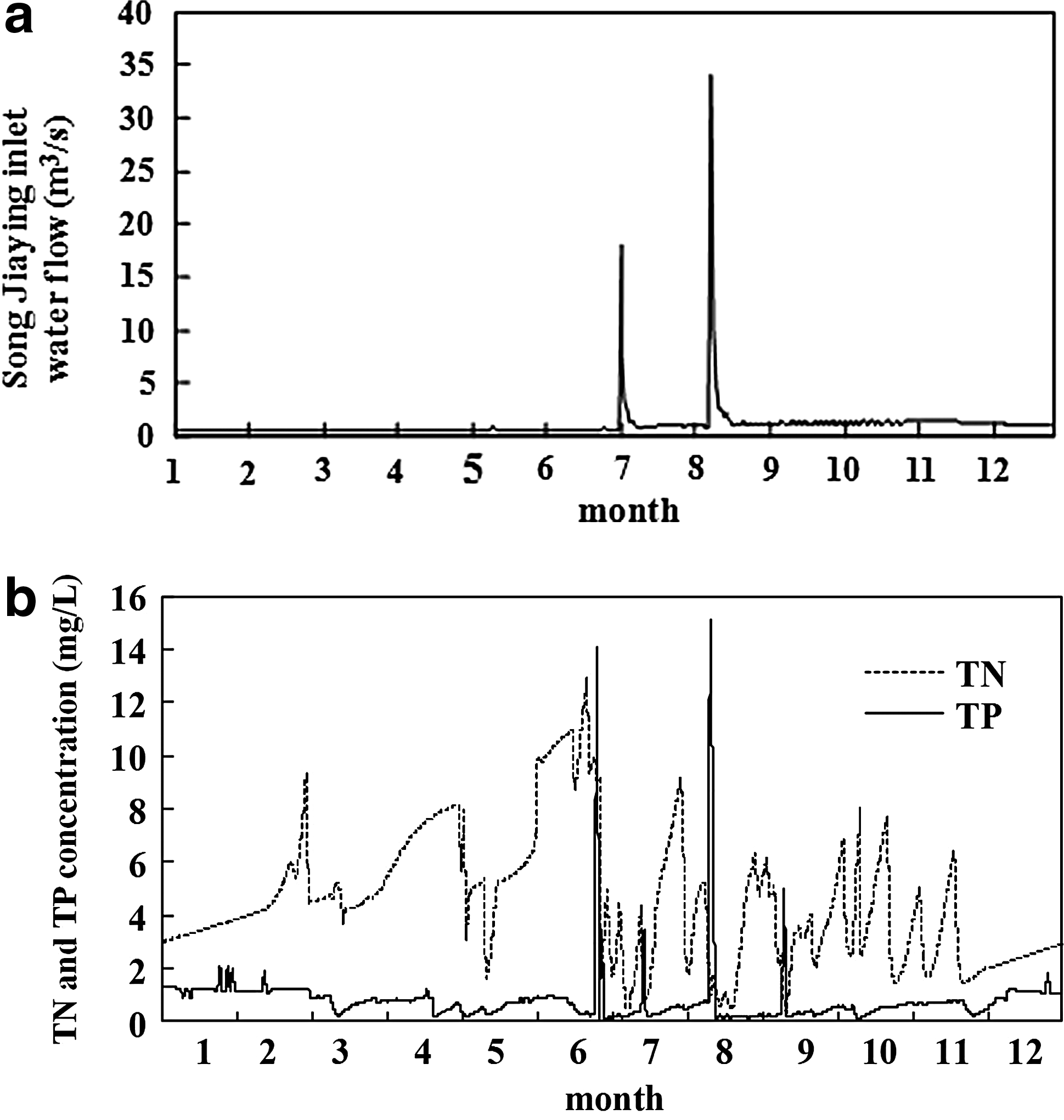
Boundary conditions at the Song Jiaying inlet during 2008. (a) Water flow at the Song Jiaying inlet. (b) TN and TP concentrations.

Riverbed roughness is the main parameter that must be calibrated, and the roughness ranged from 0.016 to 0.030. The coefficient of eddy viscosity was calculated using Smagorinsky equations. The dispersion coefficient is associated with grid spacing and local current speed. By comparing simulated and measured concentration values, the optimum empirical Elder's formulation was used to estimate dispersion coefficients of TN and TP: \documentclass{aastex}\usepackage{amsbsy}\usepackage{amsfonts}\usepackage{amssymb}\usepackage{bm}\usepackage{mathrsfs}\usepackage{pifont}\usepackage{stmaryrd}\usepackage{textcomp}\usepackage{portland, xspace}\usepackage{amsmath, amsxtra}\pagestyle{empty}\DeclareMathSizes{10}{9}{7}{6}\begin{document} \begin{align*} D = 0.03 \times \Delta x \times u , \tag{14} \end{align*} \end{document}

According to the first-order kinetics equation, decay coefficients are associated with temperatures. Comparing simulated and measured concentration values, the decay coefficient ranges for TN and TP were 7.5 × 10⁻³–1.55 × 10⁻² day⁻¹ and 8.5 × 10⁻³–1.95 × 10^–2 day⁻¹, respectively. Table 8 shows a list of the parameters and their values in this model.

Table 8.

Parameters of Coupled Two-Dimensional Model

Parameter	Description	Value
h_dry	Drying depth	0.005 m
h_flood	Flooding depth	0.05 m
h_wet	Wetting depth	0.1 m
c_s	Constant value in Smagorinsky equations of eddy viscosity	0.28
N	Bed roughness (Manning's equation)	0.016–0.030
k_TN	TN decay coefficient	7.5 × 10⁻³–1.55 × 10⁻² day⁻¹
k_TP	TP decay coefficient	8.5 × 10⁻³–1.95 × 10⁻² day⁻¹

Validation of the coupled two-dimensional model

The observation point in the central Yuqiao Reservoir (longitude 117°31′E and latitude 40°02′N) was selected as the most representative validation point of water quality. Comparisons were made between simulated and observed TN and TP concentration density variations (Figs. 12, and 13) and the relative errors are shown in Table 9.

FIG. 12.

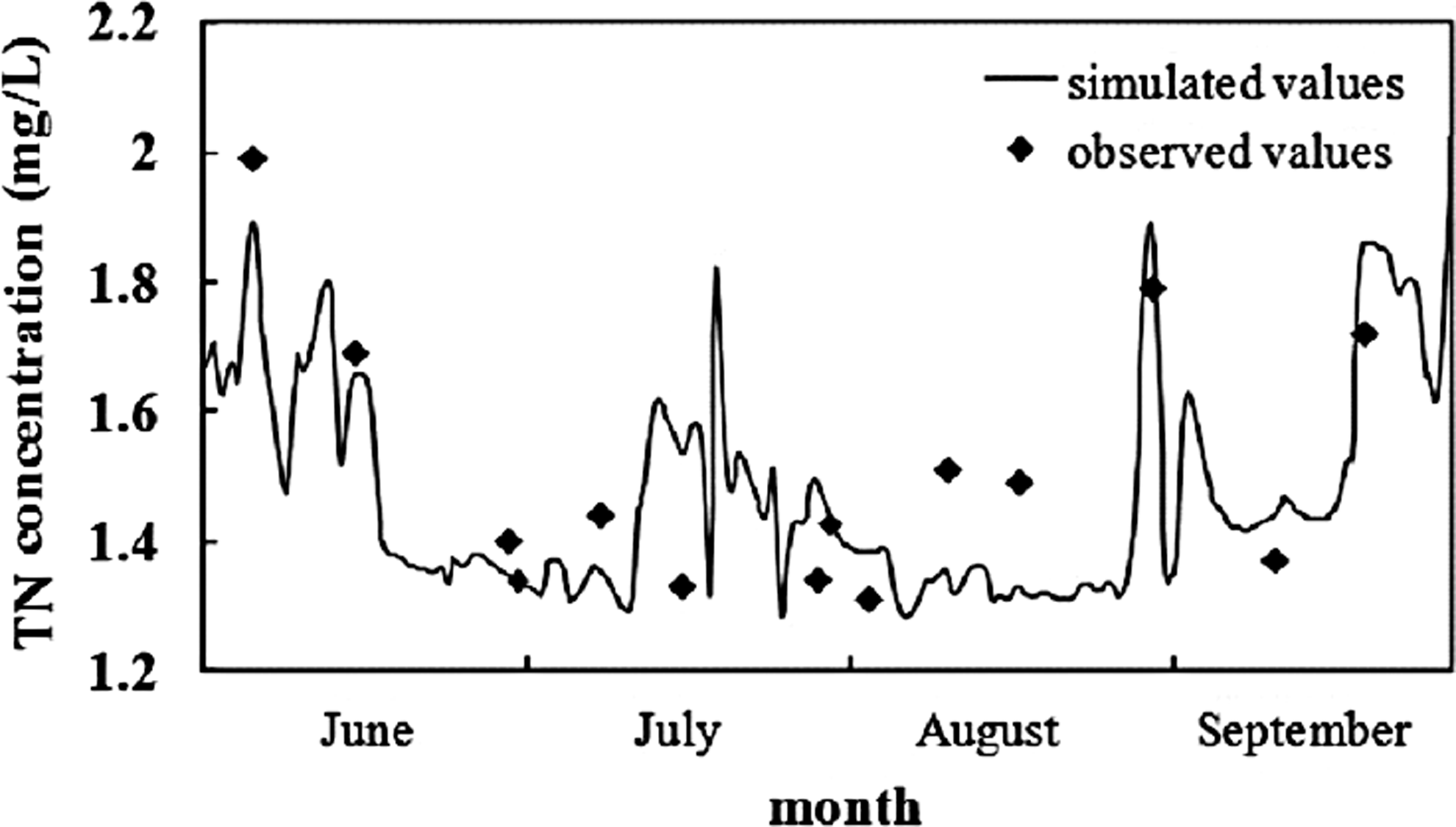
Comparison between simulated and observed TN concentrations during 2008.

FIG. 13.

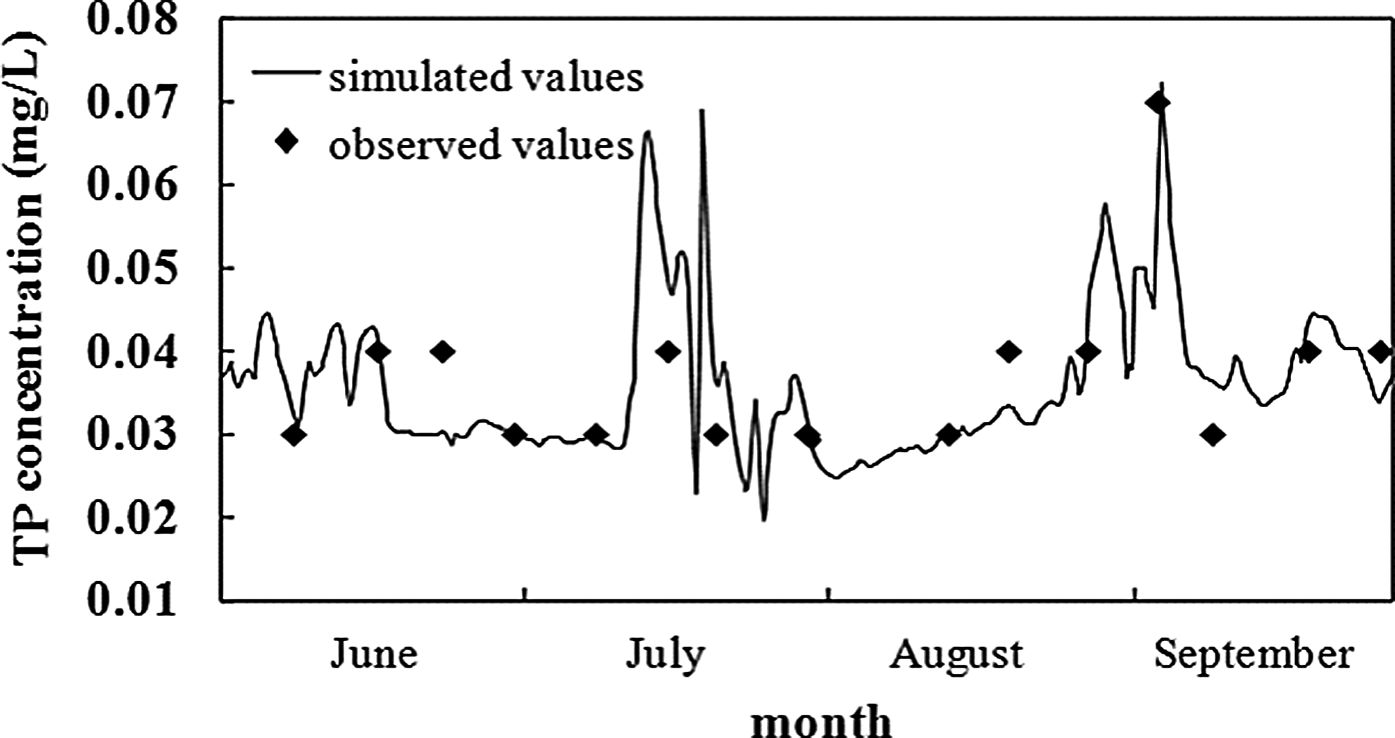
Comparison between simulated and observed TP concentrations during 2008.

Table 9.

Relative Errors of Simulated and Observed Values of Total Nitrogen and Total Phosphorus Concentrations

Date	Observed TN (mg/L)	Simulated TN (mg/L)	Relative error (%)	Date	Observed TP (mg/L)	Simulated TP (mg/L)	Relative error (%)
June 6	1.99	1.88	5.53	June 8	3.00E-02	3.15E-02	5.00
June 16	1.69	1.66	1.78	June 17	4.00E-02	4.22E-02	5.50
June 24	Null	Null	Null	June 24	3.00E-02	2.99E-02	0.33
July 1	1.40	1.35	3.57	July 1	3.00E-02	2.93E-02	2.33
July 10	1.44	1.36	5.56	July 10	4.00E-02	4.74E-02	18.50
July 18	1.33	1.52	14.29	July 17	3.00E-02	3.57E-02	19.00
July 22	Null	Null	Null	July 22	3.00E-02	3.05E-02	1.67
July 31	1.34	1.51	12.69	August 1	3.00E-02	3.05E-02	1.67
August 5	1.31	1.42	8.40	August 16	3.00E-02	2.99E-02	0.33
August 13	1.51	1.36	9.93	August 22	4.00E-02	3.33E-02	16.75
August 20	1.49	1.31	12.08	August 30	4.00E-02	4.70E-02	17.50
September 02	1.79	1.69	5.59	September 6	7.00E-02	6.31E-02	9.86
September 14	1.37	1.26	8.03	September12	3.00E-02	3.62E-02	20.67
September 22	1.72	1.56	9.30	September 22	4.00E-02	4.39E-02	9.75
September 30	Null	Null	Null	September 30	4.00E-02	3.44E-02	14.00
Average value			5.50	Average value			9.52

Figures 12 and 13 together with Table 9 show that the simulated and observed values consistently exhibited similar trends. The maximum, minimum, and average relative errors for TN were 14.29%, 1.78%, and 5.50%, respectively. The values for TP were relatively higher at 20.67%, 0.33%, and 9.52%, respectively, which were all within the acceptable error range of 30%.

Spatial and temporal distributions of TN and TP

Total nitrogen

Simulation results showed that the TN concentration was lowest in August (average value of 1.56 mg/L) and peaked in September (3.74 mg/L). In June and July, the value ranged from 2.23 to 2.47 mg/L. This temporal distribution was due to increases in precipitation and rainfall frequency in August, causing the reservoir water volume to increase that in turn reduced the TN concentration. In September, the TN concentration density in water diverted from the Luan He River was 3.0 to 5.6 mg/L, which had a large influence on the Yuqiao Reservoir water quality.

High TN concentrations were gradually transported and diffused downstream (Fig. 14a). Under the effect of small flow fields, TN in the south central reservoir showed a decreasing trend. The pollution zone shown in Figure 14a was significantly diffused in July (Fig. 14b). In 80% of the reservoir area, the TN ranged from 1.0 to 2.0 mg/L. However, the south rim maintained a high TN concentration. Owing to high precipitation in August (166.0 mm) and rainwash in July, the TN concentration in most parts of the Yuqiao Reservoir returned to a normal range (Fig. 14b, c). At the Guo River inlet there was a pollution zone with a high concentration along the south rim, which resulted from accumulated pollutants in upstream riverbeds that were carried by water diverted from the Luan He River (after August 10). In the northeastern part of the reservoir, TN at the Lin River inlet was already below 1.0 mg/L, and the value in the northwestern part of the reservoir remained at a high level (>4.5 mg/L) owing to livestock breeding in the surrounding areas. By the end of the Luan He River water diversion period, TN levels were decreasing and diffusing downstream through wind-driven currents and alongshore currents (Fig. 14d). Thus, the TN concentration in the central reservoir was obviously lower than that in the eastern part of the reservoir.

FIG. 14.

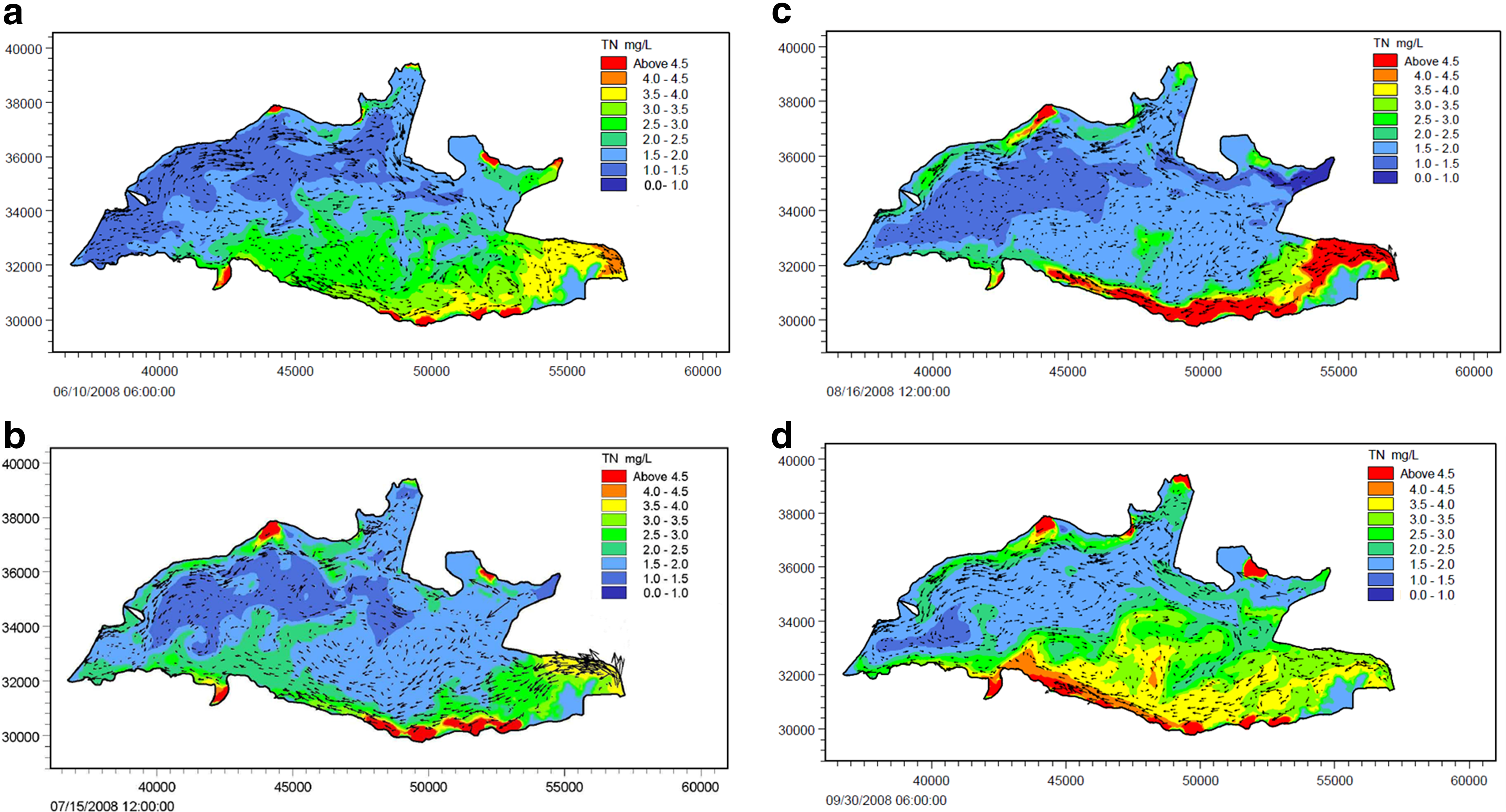
Spatial distribution of TN (mg/L) from June to September in 2008. (a) June 10, 2008. (b) July 15, 2008. (c) August 16, 2008. (d) September 30, 2008.

Spatially, the TN concentration showed a high–low–high trend from southeast to northwest, which was mainly affected by the distribution of pollutant inlets and wind-driven currents. In the northwest, nonpoint source pollutants mainly flowed into the Yuqiao Reservoir through Liu Xiangying. In the south, pollutant inlets were Wu Baihu and Huo Jiadian, which formed a high concentration pollution zone between the east and west circulations. In the northwestern and southern parts of the reservoir, the TN concentration decreased from the reservoir bank to the dam location.

In conclusion, the spatial and temporal TN distributions were mainly affected by nonpoint source pollution transported by precipitation and upstream water diverted from the Luan He River. Water quality around the reservoir was affected much more than the central reservoir. Owing to wind-driven currents, pollutants around the reservoir could influence water quality around the inlets within a short time, thus influencing the urban water supply.

Total phosphorus

Temporally, the TP concentration peaked at 4.9 × 10⁻² mg/L in July, and the value in August was slightly higher than that in June, with both values fluctuating around 3.0 × 10⁻² mg/L. The lowest concentration was in September, which had an average TP value of 2.7 × 10⁻² mg/L. The major cause of the above trends was increases in precipitation in late June when high concentrations of nonpoint source pollutants, including TP, flowed into the reservoir. By means of convection and diffusion, pollutants were gradually transferred to the central reservoir, resulting in high TP concentrations throughout the reservoir in July. Because of the heavy rainfall in August, there was a sharp increase in inflows, which diluted the waterbody. In addition, the scour of antecedent rainfalls also reduced the TP concentration. In September, inflow of water diverted from the Luan He River led to a general decrease in TP in the Yuqiao Reservoir.

Simulated TP results showed that the spatial distribution of TP was generally consistent with that of TN, however, discrepancies existed in the temporal distribution that were caused by different concentrations of TN and TP in water diverted from the Luan He River (Fig. 15).

FIG. 15.

Spatial distribution of TP (mg/L) from June to September in 2008. (a) June 10, 2008. (b) July 20, 2008. (c) August 16, 2008. (d) September 28, 2008.

The TP concentration in the east was generally higher than that in the west (Fig. 15a). Wind-driven currents had significant effects on TP diffusion. In July (Fig. 15b), highly concentrated (>0.245 mg/L) pollution zones appeared at the northwest, northeast, and south banks of the reservoir owing to large amounts of nonpoint source pollutants transported by surface runoff after heavy rainfall. Although the TP concentration in the entire reservoir declined in August (Fig. 15c), in the northeast section a pollution zone with a high TP concentration (>0.245 mg/L) appeared at the Lin River inlet. Owing to the water diverted from the Luan He River, pollutants were transported downstream along the south bank of the reservoir (Fig. 15d). Simultaneously, the concentration of TP decreased.

There was obvious spatial variability in TP in the Yuqiao Reservoir (Fig. 15). Specifically, the TP concentration increased from west to east because of the relatively low water level in the eastern part of the reservoir, which increased the water exchange rate. Moreover, owing to steep slopes and livestock breeding, the TP concentration at the south bank of the reservoir was higher than that at the north bank. Under the effects of alongshore currents, the TP concentration diffused quickly at the northwest and south banks of the reservoir, and gradually decreased downstream.

In summary, the TP temporal and spatial distributions were mainly affected by surrounding nonpoint source pollutants. Based on the TP accumulation on clear days and discharge on rainy days, precipitation was the major cause of variations in TP levels.

Discussion

Previous studies of reservoir water quality on a large scale mainly focused on the amount and transport of pollutant loads using nonpoint source pollution models (Emili and Greene, 2013; Niraula et al., 2013). At small scales, two-/three-dimensional hydrodynamic models were adopted to analyze pollutant diffusion and conversion (Han et al., 2011; Zhou et al., 2011; Zhao et al., 2012). However, these research methods were independent, and produced isolated results that may have been contradictory. Thus, combining the two methods when analyzing the production, transport and conversion of pollutants in an entire basin, is essential.

SWAT was developed to analyze the long-term impacts of land management practices on water, sediment, and agricultural chemical yields in large river basins. Although SWAT is physically based and computationally efficient, this tool applies a simple empirical model to predict the amounts of nutrients in a reservoir and thus may not meet requirements for detailed modeling of reservoir water quality. Therefore, we established a coupled two-dimensional hydrodynamic and water quality model based on Navier–Stokes equations [Eqs. (4 )–(8)] and the convection–diffusion equation [Eq. (9)]. The model was solved using an FVM, wherein all physical quantities meet the integral conservation law (Xie et al., 2014). In addition, the FVM embodies both the geometric flexibility of the finite element method and the efficiency of the finite difference method; thus, this approach is used in many computational fluid dynamics packages (Shukla et al., 2012). The linkage of the SWAT model and the two-dimensional model compensates for their deficiencies and allows for a comprehensive consideration of topography, soil properties, vegetation, weather, land management practices, hydrodynamics, and water quality in a study of water pollution in the Yuqiao Reservoir.

Although the combination of the two models offers an effective way to analyze water pollution, it requires a large amount of data. Data precision and density have direct influences on the degree of accuracy of pollution simulations. During data collection in this study, we found that water quality data in China were available for short periods and often had long intervals between observations (2 weeks to 2 months). In addition, some records were incomplete, and monitoring methods varied among different institutions in different periods. Therefore, the monitoring frequency should be increased and monitoring methods should be standardized in the near future.

Further studies of nonpoint source pollution should emphasize model optimization and data management. Researchers should also take advantage of remote sensing, geographic information systems, and global positioning systems, which can provide abundant data for numerical models that will in turn improve the accuracy of water pollution prediction.

Conclusions

Average annual inflows of TN and TP around the Yuqiao Reservoir in 2008 were 2,014.6 and 152.8 tons, respectively, of which the main sources were upstream water diversion and feces from residents and livestock.

In the model validation, relative errors between the simulated and observed concentrations of TN and TP were within an acceptable range; thus, the coupled two-dimensional model could be adopted to simulate the temporal and spatial TN and TP variations during the rainy season (June to September) in 2008.

Simulation results showed that the TN concentration peaked in September and was lowest during August. The water quality around the Yuqiao Reservoir was significantly affected by nonpoint source pollutants transported by wind-driven currents. Liu Xiangying, Wu Baihu, and Huo Jiadian were the main reservoir inlets for TN. The TP concentration peaked in July and was lowest in September. Spatially, the TP concentration in the east was generally higher than that in the west, and the south bank was the major TP inlet.

Footnotes

Acknowledgments

This study was supported by the National Natural Science Foundation of China (Grant Nos. 51179117 and 51438009) and the National Water Pollution Control and Treatment Science and Technology Major Project (Grant No. 2014ZX07203-009).

Author Disclosure Statement

No competing financial interests exist.

References

Abbaspour

K.C.

, Vejdani

, and Haghighat

(2007). SWAT-CUP calibration and uncertainty programs for SWAT. In Modsim International Congress on Modelling & Simulation Land Water & Environmental Management Integrated Systems for Sustainability. MODSIM 2007 International Congress on Modelling and Simulation, Modelling and Simulation Society of Australia and New Zealand, Vol. 364, 1603.

Abbaspour

K.C.

, Rouholahnejad

, Vaghefi

, Srinivasan

, Yang

, and Kløve

(2015). A continental-scale hydrology and water quality model for Europe: Calibration and uncertainty of a high-resolution large-scale SWAT model. J. Hydrol., 524, 733.

Baker

T.J.

, and Miller

S.N.

(2013). Using the Soil and Water Assessment Tool (SWAT) to assess land use impact on water resources in an East African watershed. J. Hydrol., 486, 100.

Chen

, Liu

R.M.

, Huang

, Chen

Y.X.

, Gao

S.H.

, Sun

C.C.

, and Shen

Z.Y.

(2013). Integrated assessment of nonpoint source pollution of a drinking water reservoir in a typical acid rain region. Int. J. Environ. Sci. Technol., 10, 651.

Chen

Y.Y.

, Zhang

, Gao

X.P.

, and Wang

L.Y.

(2012). Long-term variations of water quality in a reservoir in China. Water Sci. Technol., 65, 1454.

Emili

L.A.

, and Greene

R.P.

(2013). Modeling agricultural nonpoint source pollution using a geographic information system approach. Environ. Manage., 51, 70.

Han

, Li

, Wang

, Shi

, Qiao

, and Liu

(2011). Environmental capacity of nitrogen and phosphorus pollutions in Jiaozhou Bay, China: Modeling and assessing. Marine Pollut. Bull., 63, 262.

, Zhu

, Cao

, Li

, Zhang

, and Xie

(2015). Characteristics of early eutrophication encoded in submerged vegetation beyond water quality: A case study in Lake Erhai, China. Environ. Earth Sci., 74, 3701.

Heniche

, Secretan

, Boudreau

, and Leclerc

(2000). A two-dimensional finite element drying-wetting shallow water model for Water Resources. Adv. Water Resour., 23, 359.

10.

Lee

, Park

, Lee

, and Kim

(2010). Evaluation of non-point source pollution reduction by applying best management practices using a SWAT model and QuickBird high resolution satellite imagery. J. Environ. Sci., 22, 826.

11.

J.K.

, Li

H.E.

, Shen

, and Li

Y.J.

(2011). Effect of non-point source pollution on water quality of the Weihe River. Int. J. Sediment Res., 26, 50.

12.

, Xu

, Zhao

, Shi

, Wang

Z.L.

, and Wang

(2015). Assessing threshold values for eutrophication management using Bayesian method in Yuqiao Reservoir, North China. Environ. Monit. Assess., 187, 1.

13.

Liu

X.B.

, Peng

W.Q.

, He

G.J.

, Liu

J.L.

, and Wang

Y.C.

(2008). A coupled model of hydrodynamics and water quality for Yuqiao reservoir in Haihe river basin. J. Hydrodyn. Ser. B, 20, 574.

14.

Liu

, Huang

G.H.

, Liao

R.F.

, Li

Y.P.

, and Xie

Y.L.

(2013). Fuzzy two-stage non-point source pollution management model for agricultural systems—A case study for the Lake Tai Basin, China. Agric. Water Manage., 121, 27.

15.

Liu

, Wang

, Shi

, Chen

, Sun

, Zhang

, and Shen

(2014). Runoff characteristics and nutrient loss mechanism from plain farmland under simulated rainfall conditions. Sci. Total Environ., 468, 1069.

16.

, Li

, Zhang

, Zheng

, and Du

(2011). Assessment and analysis of non-point source nitrogen and phosphorus loads in the Three Gorges Reservoir Area of Hubei Province, China. Sci. Total Environ., 412, 154.

17.

Niraula

, Kalin

, Srivastava

, and Anderson

C.J.

(2013). Identifying critical source areas of nonpoint source pollution with SWAT and GWLF. Ecol. Model., 268, 123.

18.

Ongley

E.D.

, Xiaolan

, and Tao

(2010). Current status of agricultural and rural non-point source pollution assessment in China. Environ. Pollut., 158, 1159.

19.

Owens

L.B.

, Shipitalo

M.J.

, and Bonta

J.V.

(2008). Water quality response times to pasture management changes in small and large watersheds. J. Soil Water Conservation., 63, 292.

20.

Roe

P.L.

, and Baines

M.J.

(1982). Algorithms for advection and shock problems. In Viviand

, Ed., Numerical Methods in Fluid Mechanics. Proceedings of the 4th GAMM Conference on Numerical Methods in Fluid Mechanics, Vieweg, Braunschweig, Vol. 1. pp. 281–290.

21.

Shen

, Chen

, Liao

, Liu

, and Hong

(2012a). Impact of spatial rainfall variability on hydrology and nonpoint source pollution modeling. J. Hydrol., 472, 205.

22.

Shen

, Liao

, Hong

, and Gong

(2012b). An overview of research on agricultural non-point source pollution modelling in China. Separation Purif. Technol., 84, 104.

23.

Shen

, Qiu

, Hong

, and Chen

(2014). Simulation of spatial and temporal distributions of non-point source pollution load in the Three Gorges Reservoir Region. Sci. Total Environ., 493, 138.

24.

Shukla

, Singh

A.K.

, and Singh

(2012). A comparative study of finite volume method and finite difference method for convection-diffusion problem. Am. J. Comput. Appl. Math., 1, 67.

25.

Sweby

P.K.

(1984). High resolution schemes using flux limiters for hyperbolic conservation laws. SIAM J. Numer. Anal., 21, 995.

26.

Wellen

, Arhonditsis

G.B.

, Long

, and Boyd

(2014). Quantifying the uncertainty of nonpoint source attribution in distributed water quality models: A Bayesian assessment of SWAT's sediment export predictions. J. Hydrol., 519, 3353.

27.

, and Chen

(2013). Investigating the effects of point source and nonpoint source pollution on the water quality of the East River (Dongjiang) in South China. Ecol. Indicators, 32, 294.

28.

Xie

, Ii

, Ikebata

, and Xiao

(2014). A multi-moment finite volume method for incompressible navier–stokes equations on unstructured grids: Volume-average/point-value formulation. J. Compu. Phys., 277, 138.

29.

Zhang

G.H.

, Liu

G.B.

, Wang

G.L.

, and Wang

Y.X.

(2011). Effects of vegetation cover and rainfall intensity on sediment-bound nutrient loss, size composition and volume fractal dimension of sediment particles. Pedosphere, 21, 676.

30.

Zhang

, Liu

, Pan

, and Yu

(2013). Land use pattern optimization based on CLUE-S and SWAT models for agricultural non-point source pollution control. Math. Comput. Model., 58, 588.

31.

Zhao

D.H.

, Qi

, Yu

W.D.

, Xu

B.H.

, and Pei

Z.P.

(2000). Finite volume method and Riemann solver for depth-averaged two-dimensional flow-pollutants coupled model. Adv. Water Sci. 11, 368 (in Chinese with English abstract).

32.

Zhao

D.H.

, Yao

, Jiang

, Yang

, and Pang

(2002). FVS scheme in 2-D depth-averaged flow-pollutants modeling. Adv. Water Sci. 13, 701 (in Chinese with English abstract).

33.

Zhao

, Zhang

, Liu

, He

, Zhu

, Zou

, and Zhu

(2012). Three-dimensional hydrodynamic and water quality model for TMDL development of Lake Fuxian, China. J. Environ. Sci., 24, 1355.

34.

Zhou

, Westrich

, Jiang

, and Wang

(2011). A coupling simulation based on a hydrodynamics and water quality model of the Pearl River Delta, China. J. Hydrol., 396, 267.

35.

Zhu

(2011). Study on Agricultural Non-point Source Loads of Haihe River Basin and Assessment on Its Environmental Impact. Doctoral dissertation, Chinese Academy of Agricultural Sciences, Beijing, China (in Chinese with English abstract).

36.

Zhu

Q.D.

, Sun

J.H.

, Hua

G.F.

, Wang

J.H.

, and Wang

(2015). Runoff characteristics and non-point source pollution analysis in the Taihu Lake Basin: A case study of the town of Xueyan, China. Environ. Sci. Pollut. Res., 22, 15029.