Modeling Fluctuation of PM 10 Data with Existence of Volatility Effect

Abstract

Modeling time series data of particulate matter (PM) will provide a good understanding about the dynamic behavior of this pollution variable. In fact, a suitable model can be used as a practical tool for planning purposes and controlling adverse effects of air pollution. This article utilized an autoregressive integrated moving average (ARMA) with the combination of generalized autoregressive conditional heteroscedastic (ARCH/GARCH) to provide a suitable model that can overcome the problematic volatility effect that exists in the PM₁₀ data. Hourly PM₁₀ data for the city of Kuala Lumpur have been analyzed. Based on several statistical approaches, such as the autocorrelation function, R² coefficient, and Akaike's Information Criterion, an ARMA(1,0)-GARCH(1,1) has been determined to be the best model to describe the data. In fact, incorporation of GARCH(1,1) is able to improve forecasting performance of PM₁₀ data, instead of relying on only a single ARMA(1,0) model.

Introduction

Air quality is an important aspect that affects most human activities. To determine the status of air quality in a particular area, particulate matter (PM) data have been collected by countries around the world. PM can cause many environmental problems, particularly health hazards, and can also affect daily human activities. Hooyberghs et al. (2005) mentioned that the effects of PM on air pollution have become a well-recognized problem in environmental science. Particularly, PM can provide a direct impact on human health through inhalation (Chow et al., 2002). In fact, many studies have indicated a significant relationship between health effects and elevated concentrations of PM. For example, a study by Sanhueza et al. (2005) in Temuco, Chile has found a strong relationship between PM₁₀ and daily mortality cases (1997–2002) among subjects over 65 years old. They found that for respiratory mortality the relative risk was 1.236 times higher for every increase in PM₁₀ by 100 μg/m³ and 1.176 times higher for every increase in PM₁₀ by 100 μg/m³ for cardiovascular mortality.

Goldberg et al. (2003) and Bell et al. (2004) also have indicated a positive association between short-term variations in PM and daily mortality counts. Apart from that, a time series study of PM, mortality, and morbidity has provided evidence that daily variations in air pollution levels are associated with daily variations in mortality counts (Peng et al., 2006). In fact, increased mortality and morbidity in communities with elevated PM concentrations have been reported by a variety of epidemiological studies (for example, see Sanhueza et al., 2005; Pope and Dockery, 2006). Furthermore, PM has a wider impact on climate, causing direct (absorbing, reflecting, and scattering), indirect (clouds formation, clouds albedo and lifetime), and semidirect (heating and cooling) effects on the global radiative budget (Tiwari et al., 2012).

In Malaysia, PM₁₀ is known as one of the dominant pollutants in the country. Previous researchers have stated that this harmful pollutant is associated with haze events, industrial activity, heating, and also from vehicular traffic, provided by primary and secondary emissions from exhausts and from suspended dust on the streets generated by circulation. High concentration levels of PM₁₀ are often recorded during the dry season, especially in urbanized areas such as Kuala Lumpur. In fact, geographical positions, high industrial and commercial activities, high density populations, heavy vehicular activities, and stable atmospheric conditions (prevailing winds) were among the related factors that contributed to the problem of high levels of PM₁₀ (Afroz et al., 2003).

This study tries to provide a time series model that can be useful in predicting the stochastic behaviors of PM₁₀ particularly in the area of Kuala Lumpur. As mentioned by Perez and Reyes (2006), it will be very convenient to construct a reliable forecasting model for the data of PM₁₀ for a particular city, which can become an important information source for the authorities to warn the population about adverse conditions.

Study Areas and Data

Kuala Lumpur is the main city in Malaysia and has an approximate area of 243 km². It also has a dense population. The surrounding urban areas in Kuala Lumpur provide the most industrialized and fastest growing economical region in Malaysia. As mentioned by The World According to GaWC 2008 (2009), Kuala Lumpur has been rated as an alpha world city among the global cities in Malaysia. In fact, the development of the infrastructure in its surrounding areas, such as the creation of the Mass Rapid Transit project, Multimedia Super Corridor, Kuala Lumpur International Airport, and the expansion of Port Klang, has contributed to the economic significance. Although the economic progress is very good, the risk of air pollution caused by industrial activity and congested traffic has increased (Masseran et al., 2016). Thus, it is very important to develop a reliable forecasting model for the PM₁₀ data to study their behavior. The data used in this study include the hourly PM₁₀ values for the period from January 1, 2012 to December 31, 2015. The missing data have been estimated using the method of single imputation (Masseran et al., 2013a).

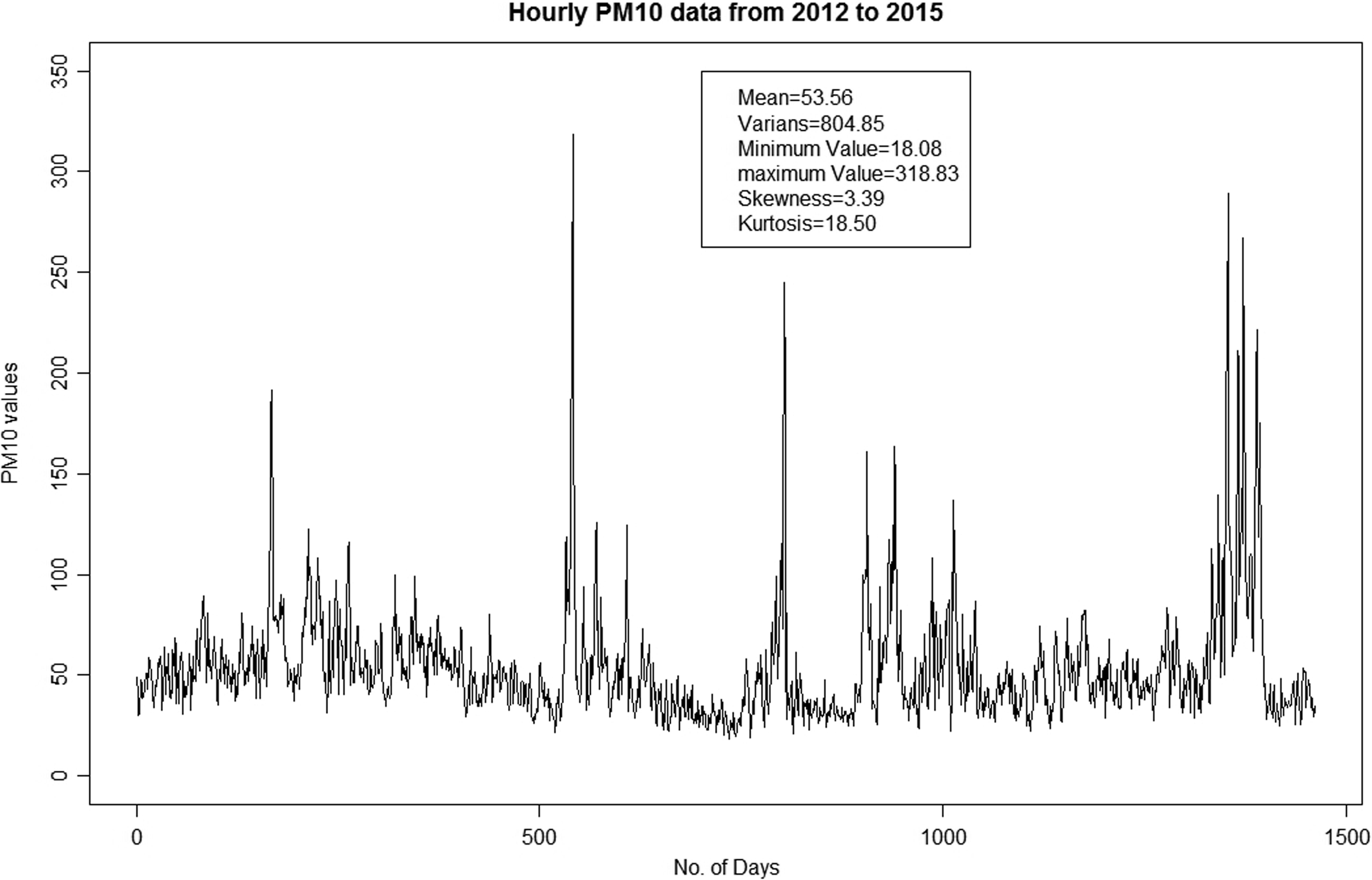
Before a detailed analysis is created, we should look at the descriptive statistics to obtain preliminary information about the PM₁₀ data in Kuala Lumpur. The descriptive statistics in Table 1 shows that the mean of PM₁₀ for the Kuala Lumpur area region is ∼53.55 μg/m³, with a standard deviation of 28.37 μg/m³. This implies that for most of the time, the value of PM₁₀ in the Kuala Lumpur areas is in the healthy limit for humans. However, the minimum and maximum value found in the period of 2012 to 2015 is 18.08 and 318.83 μg/m³, respectively, indicating that some periods of PM₁₀ data experience a very high level that negatively affects the air quality in Kuala Lumpur. In addition, the coefficient of skewness for Kuala Lumpur is not found to be zero, which indicates that the data do not follow a normal distribution. After knowing this information, the analyses begin when we explore the time series plot of the data. Fig. 1 shows the plot of the observed PM₁₀ data for Kuala Lumpur. The time series plot does not indicate any significant increasing or decreasing trends. The PM₁₀ data fluctuate around the mean level of 53.55 μg/m³, with a variance of 804.85 (μg/m³)². However, it is found that the plot shows several “shock points” that are far from its mean with an inconsistent variance. This implies the existence of the volatility effect in the PM₁₀ data.

FIG. 1.

Overall fluctuation of observed time series data for daily PM₁₀ in 2012 to 2015. PM, particulate matter.

Table 1.

Descriptive Statistics of PM₁₀ (μg/m³) Data at Kuala Lumpur Station

Station	Latitude	Longitude	Mean	Standard deviation	Min. value	Max. value	Skewness	Kurtosis
Kuala Lumpur	3°106′N	101°725′E	53.55	28.37	18.08	318.83	3.39	18.50

PM, particulate matter.

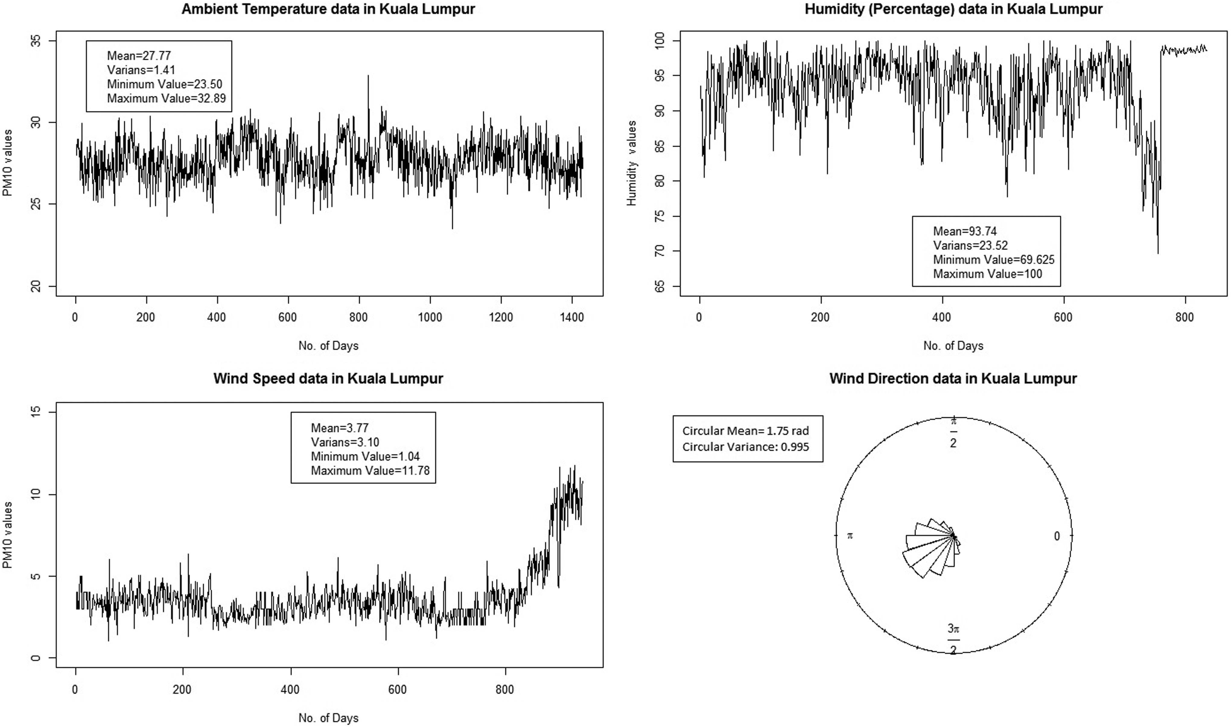
In addition, Fig. 2 describes briefly the information of other meteorological variables in Kuala Lumpur. These variables include the data of temperature, humidity, and wind speed and its direction for Kuala Lumpur area. From Fig. 2, it is found that the data of temperature are fluctuating around its mean (27.77°C) and having a small variance (1.41). These indicate that the temperature in Kuala Lumpur is quite stable. However, the humidity data in Kuala Lumpur indicate quite a large variance (23.52) with the mean of average percentage humidity being about 93.74. For wind speed, its mean (3.77 km/h) and variance (3.10) are not very high. However, the fluctuations of wind speed data are found to have an increasing trend. While the computed circular mean is about 3.66 radian (210°) and circular variance is found to be equal to 0.841, which is most of the time, the wind comes from South-West direction with a small variability toward its mean. By comparing Figs. 2 and 1, we believe that there is no significant trend between these meteorological variables which can influence the data of PM₁₀ in Kuala Lumpur.

FIG. 2.

Plots of several meteorological variables in Kuala Lumpur.

Modeling Fluctuations of PM₁₀ Data

Pollution modeling and forecasting from suspended particles in the air is obviously an important issue. The development of a statistical modeling technique of PM₁₀ concentration could be used to improve early warning procedures, particularly for sensitive people such as children, the elderly, the asthmatic patients, and so on. Thus, statistical modeling and forecasting of PM₁₀ would be an important tool for the local air quality agency to provide preliminary information and warnings to the public (Poggi and Portier, 2011). In fact, as mentioned by Diaz-Robles et al. (2008), an accurate air quality forecasting model is needed to alert the population at large and to initiate preventative pollution control actions. In addition, the application of a statistical model to evaluate the PM₁₀ data does not require a high cost, which implies a cost-effective tool to the public authorities.

A popular technique in modeling time series of air pollution data includes a class of techniques known as autoregressive moving average (ARMA) or Box–Jenkins models (Milionis and Davies, 1994; Shi and Harrison, 1997) and structural models (Schlink et al., 1997). For examples, Goyal et al. (2006) make a comparison of three statistical models which is multiple linear regression (model 1), ARIMA model (model 2), and combination of regression with ARIMA (model 3) to forecast the air quality in Delhi and Hong Kong. Their analysis found that model 3 is a better model to provide a reliable prediction for air quality. Diaz-Robles et al. (2008) have proposed a hybrid ARIMA-artificial neural network (ANN) model to forecast the air quality. They found that the ARIMA-ANN model is able to provide a good result of forecasting for the data of air quality in Temuco, Chile. Apart from that, there are many research studies that have shown that a statistical modeling and analysis is very important in providing the forecasting of air quality at a particular area.

Apart from that, some authors also mentioned about the strength of generalized autoregressive conditional heteroscedastic (GARCH) model in describing the volatility effect in the air pollution data. For example, Reisen et al. (2014) consider the seasonal autoregressive integrated moving average (SARIMA) with GARCH innovation to model the daily average of PM₁₀ data in Cariacica, Brazil. Their model is found to be able to capture the dynamics of the series that has the long memory and conditional variance. Kumar and Ridder (2010) have used GARCH modeling technique in association with fast Fourier transform (FFT)-ARIMA to forecast the daily maximum of O₃ concentration. They found that the O₃ modeling using GARCH-FFT-ARIMA will improve the short-term forecast confidence intervals. In fact, the model also provides more accurate short-term probability forecast.

ARMA and Box–Jenkins approaches are widely applied in modeling air-quality data. Although these models are quite flexible as they can represent several different types of time series, their major limitation is the presumed linear form of the model. The information about the linearity is not always reasonable for specific data. Particularly, the air pollution data exhibit a tendency to be influenced by the volatility effect. Volatility can be regarded as a measure of the variation in the fluctuations in time series data. Volatility is defined as a conditional standard deviation of the underlying time series data.

Generally, the PM₁₀ data with volatility effect indicate inconsistent variations across time. The data will show several “shock points” that are far from its mean. These shock points correspond to the pollution events which are found in a particular time. Each cluster indicates a higher variance compared to other data. This phenomenon is defined as volatility effects in a fluctuation of PM₁₀ data, not an outlier. Particularly for the Malaysian data, the occurrence of a haze event always provides a shock point in the data of PM₁₀. This knowledge should not be ignored when modeling the fluctuations of the PM₁₀ data. Thus, a time series model that combines the knowledge of the ARMA model and can capture the volatility effect on the fluctuations of air pollution data needs to be considered. In this study, the ARMA model will be combined with the generalized autoregressive conditional heteroscedastic (ARCH/GARCH) model to overcome the problem of the volatility effect that exists in the air pollution data.

Single ARMA model

ARMA is a popular model for time series data in every field of research, including air pollution data. This model comprises the autoregressive (AR) process and the moving average (MA) process. The AR processes describe the behaviors of time series data in terms of linear dependence structure. The current value of the time series, x_t, for t = 1, 2, 3, …, T can be explained based on the past p-values of the series, which we can translate in terms of PM₁₀ data. The current daily PM₁₀ data can be explained by looking back at the previous p-values of the daily PM₁₀ data. The mathematical formulation, or the p-th order of the AR model, will satisfy the following equation: \documentclass{aastex}\usepackage{amsbsy}\usepackage{amsfonts}\usepackage{amssymb}\usepackage{bm}\usepackage{mathrsfs}\usepackage{pifont}\usepackage{stmaryrd}\usepackage{textcomp}\usepackage{portland, xspace}\usepackage{amsmath, amsxtra}\usepackage{upgreek}\pagestyle{empty}\DeclareMathSizes{10}{9}{7}{6}\begin{document} \begin{align*} {x_t} = \mu + { \alpha _1}{x_{t - 1}} + { \alpha _2}{x_{t - 2}} + \ldots + + { \alpha _p}{x_{t - p}} + { \varepsilon _t} \tag{1} \end{align*} \end{document}

Apart from AR model, the time series data also can be represented in terms of MA process. The MA process describes the fluctuations of time series data using the following equation: \documentclass{aastex}\usepackage{amsbsy}\usepackage{amsfonts}\usepackage{amssymb}\usepackage{bm}\usepackage{mathrsfs}\usepackage{pifont}\usepackage{stmaryrd}\usepackage{textcomp}\usepackage{portland, xspace}\usepackage{amsmath, amsxtra}\usepackage{upgreek}\pagestyle{empty}\DeclareMathSizes{10}{9}{7}{6}\begin{document} \begin{align*} &{x_t} = \mu + {a_t} - { \beta _1}{a_{t - 1}} - { \beta _2}{a_{t - 2}} - \ldots - { \beta _q}{a_{t - q}}\\ &\quad = \mu + \mathop \sum \limits_{j = 0}^ \infty {{ \beta _j}}{a_{t - j}} \tag{2} \end{align*} \end{document}

The ARMA model has been derived by combining the information contained in the MA and AR model. In this study, time series, x_t, for the PM₁₀ data at time t is assumed to follow an ARMA (p, q) model if it satisfies the following equation: \documentclass{aastex}\usepackage{amsbsy}\usepackage{amsfonts}\usepackage{amssymb}\usepackage{bm}\usepackage{mathrsfs}\usepackage{pifont}\usepackage{stmaryrd}\usepackage{textcomp}\usepackage{portland, xspace}\usepackage{amsmath, amsxtra}\usepackage{upgreek}\pagestyle{empty}\DeclareMathSizes{10}{9}{7}{6}\begin{document} \begin{align*} & {x_t} = E \left( {{x_t} \ \vert \ {F_{t - 1}}} \right) + { \varepsilon _t} \\ &\quad = \mu + \mathop \sum \limits_{i = 1}^p {{ \alpha _i}{x_{t - i}}} - \mathop \sum \limits_{j = 1}^q {{ \beta _j}{a_{t - j}}} + { \varepsilon _t} \\ &\quad = \mu + \alpha \left( { \bf{{B}}} \right) {x_t} + \beta \left( { \bf{{B}}} \right) {a_t} + { \varepsilon _t} \tag{3} \end{align*} \end{document}

where \documentclass{aastex}\usepackage{amsbsy}\usepackage{amsfonts}\usepackage{amssymb}\usepackage{bm}\usepackage{mathrsfs}\usepackage{pifont}\usepackage{stmaryrd}\usepackage{textcomp}\usepackage{portland, xspace}\usepackage{amsmath, amsxtra}\usepackage{upgreek}\pagestyle{empty}\DeclareMathSizes{10}{9}{7}{6}\begin{document} $$\mu$$ \end{document} is a mean of the ARMA model, \documentclass{aastex}\usepackage{amsbsy}\usepackage{amsfonts}\usepackage{amssymb}\usepackage{bm}\usepackage{mathrsfs}\usepackage{pifont}\usepackage{stmaryrd}\usepackage{textcomp}\usepackage{portland, xspace}\usepackage{amsmath, amsxtra}\usepackage{upgreek}\pagestyle{empty}\DeclareMathSizes{10}{9}{7}{6}\begin{document} $${ \alpha _i}$$ \end{document} is a parameter for the AR component, \documentclass{aastex}\usepackage{amsbsy}\usepackage{amsfonts}\usepackage{amssymb}\usepackage{bm}\usepackage{mathrsfs}\usepackage{pifont}\usepackage{stmaryrd}\usepackage{textcomp}\usepackage{portland, xspace}\usepackage{amsmath, amsxtra}\usepackage{upgreek}\pagestyle{empty}\DeclareMathSizes{10}{9}{7}{6}\begin{document} $${ \beta _j}$$ \end{document} is a parameter for the MA component, \documentclass{aastex}\usepackage{amsbsy}\usepackage{amsfonts}\usepackage{amssymb}\usepackage{bm}\usepackage{mathrsfs}\usepackage{pifont}\usepackage{stmaryrd}\usepackage{textcomp}\usepackage{portland, xspace}\usepackage{amsmath, amsxtra}\usepackage{upgreek}\pagestyle{empty}\DeclareMathSizes{10}{9}{7}{6}\begin{document} $${ \bf{{B}}}$$ \end{document} is a backward shift operator which is defined as \documentclass{aastex}\usepackage{amsbsy}\usepackage{amsfonts}\usepackage{amssymb}\usepackage{bm}\usepackage{mathrsfs}\usepackage{pifont}\usepackage{stmaryrd}\usepackage{textcomp}\usepackage{portland, xspace}\usepackage{amsmath, amsxtra}\usepackage{upgreek}\pagestyle{empty}\DeclareMathSizes{10}{9}{7}{6}\begin{document} $${ \bf{{B}}}{x_t} = {x_{t - 1}}$$ \end{document} and \documentclass{aastex}\usepackage{amsbsy}\usepackage{amsfonts}\usepackage{amssymb}\usepackage{bm}\usepackage{mathrsfs}\usepackage{pifont}\usepackage{stmaryrd}\usepackage{textcomp}\usepackage{portland, xspace}\usepackage{amsmath, amsxtra}\usepackage{upgreek}\pagestyle{empty}\DeclareMathSizes{10}{9}{7}{6}\begin{document} $${ \varepsilon _t}$$ \end{document} of the residual of the model. The function \documentclass{aastex}\usepackage{amsbsy}\usepackage{amsfonts}\usepackage{amssymb}\usepackage{bm}\usepackage{mathrsfs}\usepackage{pifont}\usepackage{stmaryrd}\usepackage{textcomp}\usepackage{portland, xspace}\usepackage{amsmath, amsxtra}\usepackage{upgreek}\pagestyle{empty}\DeclareMathSizes{10}{9}{7}{6}\begin{document} $$\alpha \left( { \bf{{B}}} \right)$$ \end{document} and \documentclass{aastex}\usepackage{amsbsy}\usepackage{amsfonts}\usepackage{amssymb}\usepackage{bm}\usepackage{mathrsfs}\usepackage{pifont}\usepackage{stmaryrd}\usepackage{textcomp}\usepackage{portland, xspace}\usepackage{amsmath, amsxtra}\usepackage{upgreek}\pagestyle{empty}\DeclareMathSizes{10}{9}{7}{6}\begin{document} $$\beta \left( { \bf{{B}}} \right)$$ \end{document} are the -+polynomials of degree p and q with respect to the backward shift operator \documentclass{aastex}\usepackage{amsbsy}\usepackage{amsfonts}\usepackage{amssymb}\usepackage{bm}\usepackage{mathrsfs}\usepackage{pifont}\usepackage{stmaryrd}\usepackage{textcomp}\usepackage{portland, xspace}\usepackage{amsmath, amsxtra}\usepackage{upgreek}\pagestyle{empty}\DeclareMathSizes{10}{9}{7}{6}\begin{document} $${ \bf{{B}}}$$ \end{document} (Wurtz et al. [forthcoming]). In addition, if q = 0, an ARMA model will become a pure AR process, but if p = 0, it will become a pure MA process. In some situations, if the time series data are not stationary, it needs to be transformed using the difference method, which requires \documentclass{aastex}\usepackage{amsbsy}\usepackage{amsfonts}\usepackage{amssymb}\usepackage{bm}\usepackage{mathrsfs}\usepackage{pifont}\usepackage{stmaryrd}\usepackage{textcomp}\usepackage{portland, xspace}\usepackage{amsmath, amsxtra}\usepackage{upgreek}\pagestyle{empty}\DeclareMathSizes{10}{9}{7}{6}\begin{document} $${z_t} = {x_t} - {x_{t - 1}}$$ \end{document} for the first difference, \documentclass{aastex}\usepackage{amsbsy}\usepackage{amsfonts}\usepackage{amssymb}\usepackage{bm}\usepackage{mathrsfs}\usepackage{pifont}\usepackage{stmaryrd}\usepackage{textcomp}\usepackage{portland, xspace}\usepackage{amsmath, amsxtra}\usepackage{upgreek}\pagestyle{empty}\DeclareMathSizes{10}{9}{7}{6}\begin{document} $${z_t} = \left( {{x_t} - {x_{t - 1}}} \right) - \left( {{x_{t - 1}} - {x_{t - 2}}} \right)$$ \end{document} for the second difference, and so on. Then, a suitable ARMA model for a stationary time series can easily be determined using the plot of the autocorrelation and partial autocorrelation functions (PACFs). The formula for autocorrelation, r_k, and partial autocorrelation, \documentclass{aastex}\usepackage{amsbsy}\usepackage{amsfonts}\usepackage{amssymb}\usepackage{bm}\usepackage{mathrsfs}\usepackage{pifont}\usepackage{stmaryrd}\usepackage{textcomp}\usepackage{portland, xspace}\usepackage{amsmath, amsxtra}\usepackage{upgreek}\pagestyle{empty}\DeclareMathSizes{10}{9}{7}{6}\begin{document} $${r_{kk}}$$ \end{document} , is given as \documentclass{aastex}\usepackage{amsbsy}\usepackage{amsfonts}\usepackage{amssymb}\usepackage{bm}\usepackage{mathrsfs}\usepackage{pifont}\usepackage{stmaryrd}\usepackage{textcomp}\usepackage{portland, xspace}\usepackage{amsmath, amsxtra}\usepackage{upgreek}\pagestyle{empty}\DeclareMathSizes{10}{9}{7}{6}\begin{document} \begin{align*} { r_k } = { \frac { \mathop \sum \limits_ { t = b } ^ { n - k } { \left( { { x_t } - \bar x } \right) \left( { { x_ { t + k } } - \bar x } \right) } } { \mathop \sum \limits_ { t = b } ^ { n - k } { { { \left( { { x_t } - \bar x } \right) } ^2 } } } } \tag { 4 } \end{align*} \end{document}

and \documentclass{aastex}\usepackage{amsbsy}\usepackage{amsfonts}\usepackage{amssymb}\usepackage{bm}\usepackage{mathrsfs}\usepackage{pifont}\usepackage{stmaryrd}\usepackage{textcomp}\usepackage{portland, xspace}\usepackage{amsmath, amsxtra}\usepackage{upgreek}\pagestyle{empty}\DeclareMathSizes{10}{9}{7}{6}\begin{document} \begin{align*} {r_{kk}} = \left\{ { \begin{matrix} {{r_1} \quad \quad \quad \quad \quad if \;k = 1} \\ \begin{matrix} \hfill \\ {{{r_k} - \mathop \sum \limits_{j = 1}^{k - 1} {{r_{k - 1 , j}}{r_{k - j}}} } \over {1 - \mathop \sum \limits_{j = 1}^{k - 1} {{r_{k - 1 , j}}{r_j}} }} \quad if \;k = 2 , 3 \ldots \hfill \\\end{matrix} \\ \end{matrix}} \right. \tag{5} \end{align*} \end{document}

with \documentclass{aastex}\usepackage{amsbsy}\usepackage{amsfonts}\usepackage{amssymb}\usepackage{bm}\usepackage{mathrsfs}\usepackage{pifont}\usepackage{stmaryrd}\usepackage{textcomp}\usepackage{portland, xspace}\usepackage{amsmath, amsxtra}\usepackage{upgreek}\pagestyle{empty}\DeclareMathSizes{10}{9}{7}{6}\begin{document} $${r_{kj}} = {r_{k - 1 , j}} - {r_{kk}}{r_{k - 1 , k - j}}$$ \end{document} for \documentclass{aastex}\usepackage{amsbsy}\usepackage{amsfonts}\usepackage{amssymb}\usepackage{bm}\usepackage{mathrsfs}\usepackage{pifont}\usepackage{stmaryrd}\usepackage{textcomp}\usepackage{portland, xspace}\usepackage{amsmath, amsxtra}\usepackage{upgreek}\pagestyle{empty}\DeclareMathSizes{10}{9}{7}{6}\begin{document} $$j = 1 , 2 , 3 \ldots k - 1$$ \end{document} (Bowerman et al., 2005).

Single ARCH/GARCH model

A single ARCH/GARCH model has been designed to capture the volatility clusters in the time series data. Given the value of PM₁₀ at time t, x_t, the formula for ARCH model is given as \documentclass{aastex}\usepackage{amsbsy}\usepackage{amsfonts}\usepackage{amssymb}\usepackage{bm}\usepackage{mathrsfs}\usepackage{pifont}\usepackage{stmaryrd}\usepackage{textcomp}\usepackage{portland, xspace}\usepackage{amsmath, amsxtra}\usepackage{upgreek}\pagestyle{empty}\DeclareMathSizes{10}{9}{7}{6}\begin{document} \begin{align*} \sigma _t^2 = \omega + \mathop \sum \limits_{i = 1}^{{L_1}} {{ \gamma _i}x_{t - i}^2} \tag{6} \end{align*} \end{document}

where L₁ is the number of lags, and \documentclass{aastex}\usepackage{amsbsy}\usepackage{amsfonts}\usepackage{amssymb}\usepackage{bm}\usepackage{mathrsfs}\usepackage{pifont}\usepackage{stmaryrd}\usepackage{textcomp}\usepackage{portland, xspace}\usepackage{amsmath, amsxtra}\usepackage{upgreek}\pagestyle{empty}\DeclareMathSizes{10}{9}{7}{6}\begin{document} $${ \varphi _i}$$ \end{document} is the parameter corresponding to the value of \documentclass{aastex}\usepackage{amsbsy}\usepackage{amsfonts}\usepackage{amssymb}\usepackage{bm}\usepackage{mathrsfs}\usepackage{pifont}\usepackage{stmaryrd}\usepackage{textcomp}\usepackage{portland, xspace}\usepackage{amsmath, amsxtra}\usepackage{upgreek}\pagestyle{empty}\DeclareMathSizes{10}{9}{7}{6}\begin{document} $$\sigma _{t - j}^2$$ \end{document} . For more detail, see reference (Tsay, 2005; Danielsson, 2011).However, analysis of a single ARCH/GARCH model will only be able to capture the volatility effect in the data without considering in detail about the dynamics changing of the mean effect.

ARMA model with ARCH/GARCH residual

An ARMA and ARCH/GARCH model can provide a good basis for modeling the fluctuations of PM₁₀ data; however, we need to provide a comprehensive assessment regarding the stochastic behaviors of the PM₁₀ evaluation, which covers the dynamics changing of the mean with the volatility effect in terms of residual fluctuations. The mean effect of the time series data can be captured by ARMA model. However, the variance effects that can be described by the volatility of the data are not directly observable. The unobservability of volatility causes the evaluation of the forecasting performance of conditional heteroscedastic models to become difficult. Thus, the ARMA model was not able to provide an optimum assessment without considering the effect of the inherent volatility in the data (Masseran, 2016). To overcome that problem, the model of ARCH/GARCH needs to be combined with the ARMA model. The combination of ARMA-GARCH model will be able to govern the behavior of the mean-variance effect simultaneously in the time series data under study.

For a given ARMA residual data at time t, \documentclass{aastex}\usepackage{amsbsy}\usepackage{amsfonts}\usepackage{amssymb}\usepackage{bm}\usepackage{mathrsfs}\usepackage{pifont}\usepackage{stmaryrd}\usepackage{textcomp}\usepackage{portland, xspace}\usepackage{amsmath, amsxtra}\usepackage{upgreek}\pagestyle{empty}\DeclareMathSizes{10}{9}{7}{6}\begin{document} $$\left( {{ \varepsilon _t} = {y_t} - {{ \hat y}_t}} \right)$$ \end{document} , the idea behind the volatility study on the series of a_t is based on whether the series is either serially uncorrelated or correlated with the lower order in determination. However, the series is a dependent series. This prerequisite can easily be determined using the method of the autocorrelation function (ACF) and the PACF to the residual of the ARMA model. The GARCH model is built based on the assumption of the conditional mean and the conditional variance for a_t, given the information that is available at time t−1, \documentclass{aastex}\usepackage{amsbsy}\usepackage{amsfonts}\usepackage{amssymb}\usepackage{bm}\usepackage{mathrsfs}\usepackage{pifont}\usepackage{stmaryrd}\usepackage{textcomp}\usepackage{portland, xspace}\usepackage{amsmath, amsxtra}\usepackage{upgreek}\pagestyle{empty}\DeclareMathSizes{10}{9}{7}{6}\begin{document} $${F_{t - 1}}$$ \end{document} ; that is, \documentclass{aastex}\usepackage{amsbsy}\usepackage{amsfonts}\usepackage{amssymb}\usepackage{bm}\usepackage{mathrsfs}\usepackage{pifont}\usepackage{stmaryrd}\usepackage{textcomp}\usepackage{portland, xspace}\usepackage{amsmath, amsxtra}\usepackage{upgreek}\pagestyle{empty}\DeclareMathSizes{10}{9}{7}{6}\begin{document} \begin{align*} & {x_t} = E \left( {{x_t} \ \vert \ {F_{t - 1}}} \right) + { \varepsilon _t} \quad \quad { \rm{and}} \quad \quad { \varepsilon _t} = {z_t} \sigma _t^2\ \tag{8} \end{align*} \end{document}

The equation for \documentclass{aastex}\usepackage{amsbsy}\usepackage{amsfonts}\usepackage{amssymb}\usepackage{bm}\usepackage{mathrsfs}\usepackage{pifont}\usepackage{stmaryrd}\usepackage{textcomp}\usepackage{portland, xspace}\usepackage{amsmath, amsxtra}\usepackage{upgreek}\pagestyle{empty}\DeclareMathSizes{10}{9}{7}{6}\begin{document} $$E \left( {{x_t} \ \vert \ {F_{t - 1}}} \right)$$ \end{document} has been described using the ARMA model. Then, the variance equation of the GARCH(m,n) model can be expressed as \documentclass{aastex}\usepackage{amsbsy}\usepackage{amsfonts}\usepackage{amssymb}\usepackage{bm}\usepackage{mathrsfs}\usepackage{pifont}\usepackage{stmaryrd}\usepackage{textcomp}\usepackage{portland, xspace}\usepackage{amsmath, amsxtra}\usepackage{upgreek}\pagestyle{empty}\DeclareMathSizes{10}{9}{7}{6}\begin{document} \begin{align*} {z_t} \, \sim \, D \left( {0 , 1} \right) , \quad \sigma _t^2 = Var \left( {{ \varepsilon _t} \, \vert \, {F_{t - 1}}} \right) \tag{9} \end{align*} \end{document} \documentclass{aastex}\usepackage{amsbsy}\usepackage{amsfonts}\usepackage{amssymb}\usepackage{bm}\usepackage{mathrsfs}\usepackage{pifont}\usepackage{stmaryrd}\usepackage{textcomp}\usepackage{portland, xspace}\usepackage{amsmath, amsxtra}\usepackage{upgreek}\pagestyle{empty}\DeclareMathSizes{10}{9}{7}{6}\begin{document} \begin{align*} & \sigma _t^2 = \omega + \mathop \sum \limits_{i = 1}^m {{ \gamma _i} \varepsilon _{t - i}^2} + \mathop \sum \limits_{i = 1}^n {{ \varphi _i} \sigma _{t - i}^2}\\ &\quad = \omega + \gamma \left( { \bf{{B}}} \right) \varepsilon _{t - 1}^2 + \varphi \left( { \bf{{B}}} \right) \sigma _{t - 1}^2 \tag{10} \end{align*} \end{document}

Results and Discussion

In this study, R programming language has been used to run the analysis involving the model of ARMA-GARCH. The suitable ARMA model for the mean equation \documentclass{aastex}\usepackage{amsbsy}\usepackage{amsfonts}\usepackage{amssymb}\usepackage{bm}\usepackage{mathrsfs}\usepackage{pifont}\usepackage{stmaryrd}\usepackage{textcomp}\usepackage{portland, xspace}\usepackage{amsmath, amsxtra}\usepackage{upgreek}\pagestyle{empty}\DeclareMathSizes{10}{9}{7}{6}\begin{document} $$E \left( {{x_t} \vert {F_{t - 1}}} \right)$$ \end{document} will be determined using the ACF and the PACF. Based on Fig. 3, it is found that the ACF decreases gradually, while the PACF is truncated at lag 1.

FIG. 3.

Autocorrelation and partial autocorrelation plot for observed data. ACF, autocorrelation function.

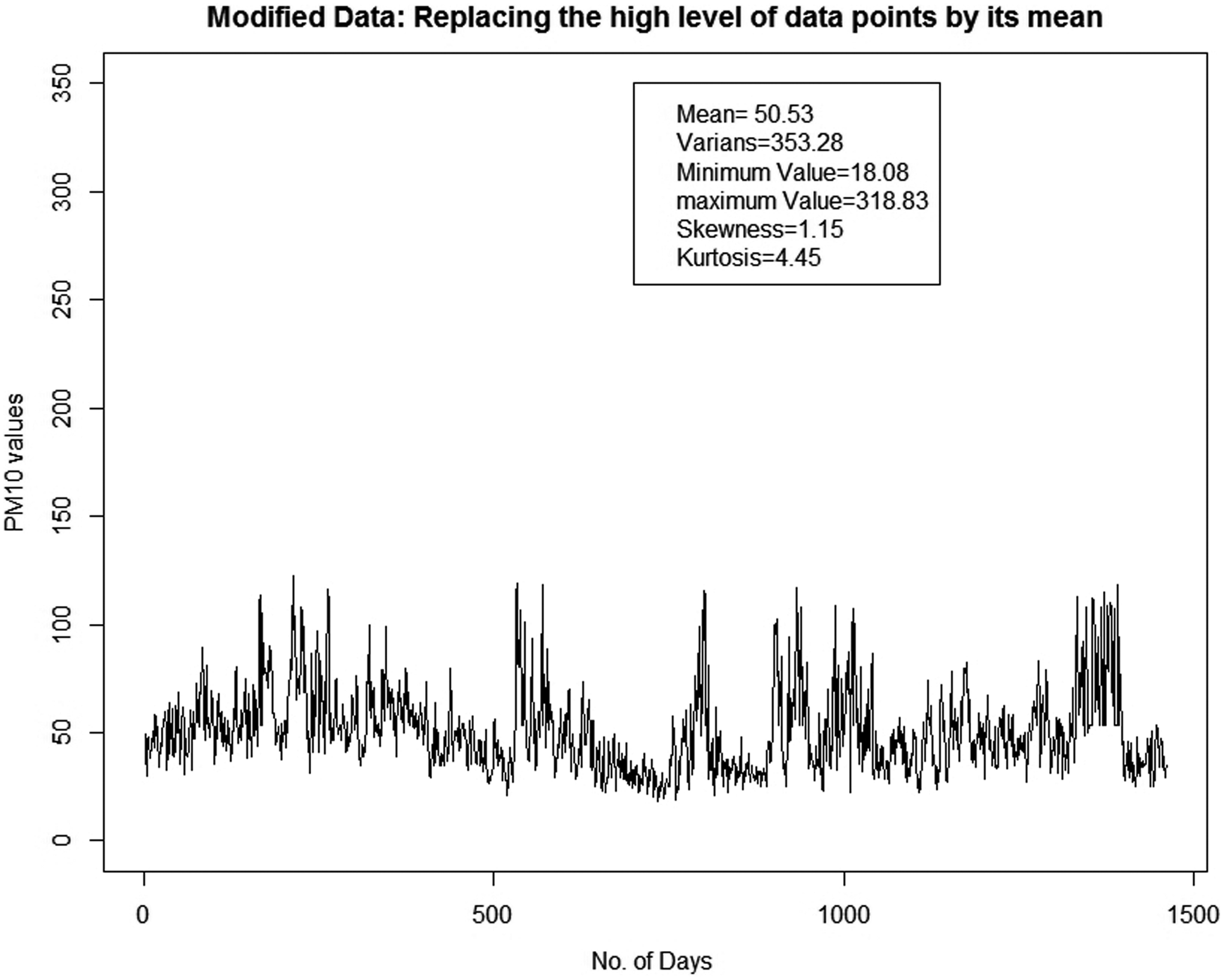
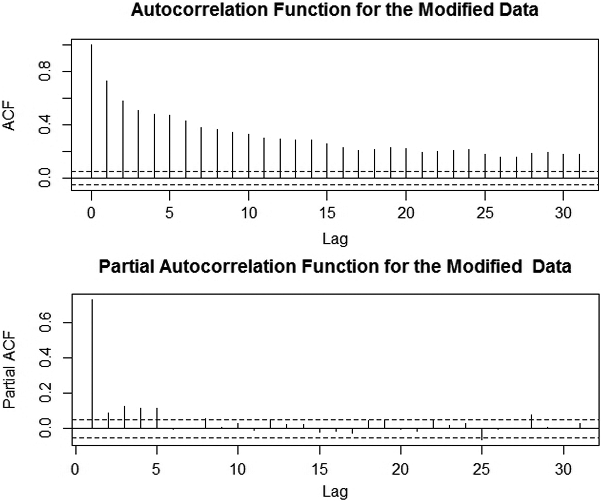
However, to investigate about the influences of the high levels of the pollutant to overall data set, we modified the original data by replacing the high levels of the pollutant by its mean. Then we also computed the ACF and PACF functions of the modified data. By considering the value of PM₁₀ > 120 as a high level of the pollutant, there exist 35 data points that exceed this level. Figure 4 shows the time series plot for the modified data. It is clear that the series of the modified data is having small and stable variances through time scale. In fact, its skewness and kurtosis values are also becoming smaller. In addition, Fig. 5 shows the ACF and PACF function for the modified data. The ACF for modified data is found to have almost the same pattern with the ACF for original data. However, the ACF for modified data is found to decrease gradually and more slowly compared to ACF for observed data, while the PACF for modified data is truncated at lag 5. These imply that the high level of data points really influences the volatility properties of the original data.

FIG. 4.

Time series plot for the modified data.

FIG. 5.

Autocorrelation and partial autocorrelation plot for modified data.

Thus, to model the observed PM₁₀ data, an ARMA(1,0) should be considered as the model for the PM₁₀ data, which is described by the mean equation. The parameter estimation for the ARMA(1,0) model was created using the maximum likelihood estimate. Thus, an estimate for the mean model that is based on the ARMA(1,0) can be written as \documentclass{aastex}\usepackage{amsbsy}\usepackage{amsfonts}\usepackage{amssymb}\usepackage{bm}\usepackage{mathrsfs}\usepackage{pifont}\usepackage{stmaryrd}\usepackage{textcomp}\usepackage{portland, xspace}\usepackage{amsmath, amsxtra}\usepackage{upgreek}\pagestyle{empty}\DeclareMathSizes{10}{9}{7}{6}\begin{document} \begin{align*} {x_t} = 53.55 + \left( {{ \rm{0}}{ \rm{.7915}}} \right) \,{x_{t - 1}} + { \varepsilon _t} , \tag{11} \end{align*} \end{document}

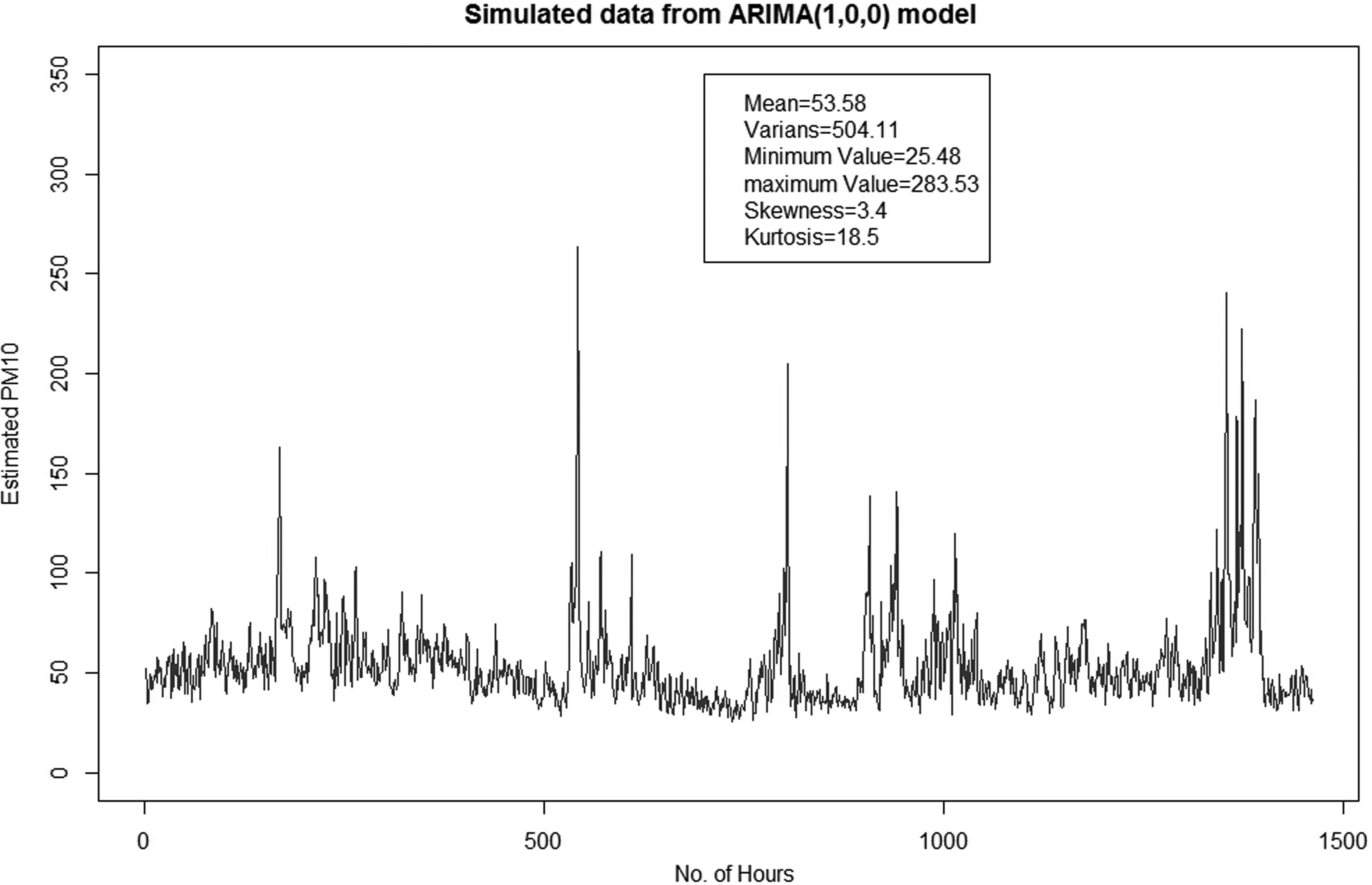
Simulated time series data from ARMA(1,0) have been generated as shown in Fig. 6. It is found that the time series plot of the data agrees with the plot for the observed data. Thus, we should consider ARMA(1,0) as a good approximation of the mean model \documentclass{aastex}\usepackage{amsbsy}\usepackage{amsfonts}\usepackage{amssymb}\usepackage{bm}\usepackage{mathrsfs}\usepackage{pifont}\usepackage{stmaryrd}\usepackage{textcomp}\usepackage{portland, xspace}\usepackage{amsmath, amsxtra}\usepackage{upgreek}\pagestyle{empty}\DeclareMathSizes{10}{9}{7}{6}\begin{document} $$E \left( {{x_t} \,\vert\, {F_{t - 1}}} \right)$$ \end{document} for PM₁₀ data in Kuala Lumpur. Based on the comparison of each statistical measurement, we found that the mean, skewness, and kurtosis provide the same value for both ARMA(1,0) and also the observed data. However, the variance, minimum value, and maximum value generated by the ARMA(1,0) model is not consistent with the value provided by the observed data. The variability for the simulated data is ∼404.11, which is much lower than that of the original data, which is 804.85. The same problem occurs for the maximum value, in which the maximum simulated data ARMA(1,0) are found to be 263.53 while the original data maximum value is ∼318.83. In contrast, the minimum value for ARMA(1,0) is 25.48, which is higher than the minimum value of original data at 18.08. The time series plot of ARMA(1,0) also clearly indicates small variability compared to the variability in the observed PM₁₀ time series plot. These problems occur because of the volatility effect in the PM₁₀ data, which implies that the modeling and forecasting of PM₁₀ data using the ARMA(1,0) model is less accurate.

FIG. 6.

Simulated time series data of PM₁₀ from ARMA(1,0) model. ARMA, autoregressive integrated moving average.

Apart from that, Fig. 7 shows the squared residual plot of the ARMA(1,0) model. This figure shows large changes that occurred occasionally, but there were also stable periods. Thus, the squared residuals for the mean model indicate the effect of volatility, which should be that the residuals can be modeled correctly by covering the volatility effect presented in the residual. However, to determine the most suitable model for ARCH/GARCH, the method of Akaike's Information Criterion (AIC) will be used.

FIG. 7.

Residual plot for volatility effect. ARCH, autoregressive conditional heteroscedastic.

Parameter estimation for the ARCH/GARCH model

Before selecting a suitable GARCH model for the residuals, it is important to determine the parameter estimation for the GARCH model. In practical applications, \documentclass{aastex}\usepackage{amsbsy}\usepackage{amsfonts}\usepackage{amssymb}\usepackage{bm}\usepackage{mathrsfs}\usepackage{pifont}\usepackage{stmaryrd}\usepackage{textcomp}\usepackage{portland, xspace}\usepackage{amsmath, amsxtra}\usepackage{upgreek}\pagestyle{empty}\DeclareMathSizes{10}{9}{7}{6}\begin{document} $${ \varepsilon _t} = \sigma _t^2{z_t}$$ \end{document} , which is equivalent to \documentclass{aastex}\usepackage{amsbsy}\usepackage{amsfonts}\usepackage{amssymb}\usepackage{bm}\usepackage{mathrsfs}\usepackage{pifont}\usepackage{stmaryrd}\usepackage{textcomp}\usepackage{portland, xspace}\usepackage{amsmath, amsxtra}\usepackage{upgreek}\pagestyle{empty}\DeclareMathSizes{10}{9}{7}{6}\begin{document} $$ { z_t } = { \frac { \sigma _t^2 } { { \varepsilon _t } } } $$ \end{document} , is often assumed to follow one of three following distributions which are given as:

(i) Standard normal distribution: \documentclass{aastex}\usepackage{amsbsy}\usepackage{amsfonts}\usepackage{amssymb}\usepackage{bm}\usepackage{mathrsfs}\usepackage{pifont}\usepackage{stmaryrd}\usepackage{textcomp}\usepackage{portland, xspace}\usepackage{amsmath, amsxtra}\usepackage{upgreek}\pagestyle{empty}\DeclareMathSizes{10}{9}{7}{6}\begin{document} \begin{align*} f \left( z \right) = \frac { 1 } { { \sqrt { 2 \pi } } } { e^ { - \frac { { { z^2 } } } { 2 } } } , \, - \infty < z < \infty \tag { 12 } \end{align*} \end{document}

(ii) Standardized Student-t distribution: \documentclass{aastex}\usepackage{amsbsy}\usepackage{amsfonts}\usepackage{amssymb}\usepackage{bm}\usepackage{mathrsfs}\usepackage{pifont}\usepackage{stmaryrd}\usepackage{textcomp}\usepackage{portland, xspace}\usepackage{amsmath, amsxtra}\usepackage{upgreek}\pagestyle{empty}\DeclareMathSizes{10}{9}{7}{6}\begin{document} \begin{align*} f \left( { z \ \vert \ v } \right) = { \frac { \Gamma \left( { \frac { { v + 1 } } { 2 } } \right) } { \sqrt { \pi \left( { v - 2 } \right) \Gamma \left( { \frac { v } { 2 } } \right) } { { \left( { 1 + { \frac { { z^2 } } { v - 2 } } } \right) } ^ { \frac { { v + 1 } } { 2 } } } } } , \ v > 2 , - \infty { \kern 1pt } < z < \infty \tag { 13 } \end{align*} \end{document}

(iii) Generalized residual distribution: \documentclass{aastex}\usepackage{amsbsy}\usepackage{amsfonts}\usepackage{amssymb}\usepackage{bm}\usepackage{mathrsfs}\usepackage{pifont}\usepackage{stmaryrd}\usepackage{textcomp}\usepackage{portland, xspace}\usepackage{amsmath, amsxtra}\usepackage{upgreek}\pagestyle{empty}\DeclareMathSizes{10}{9}{7}{6}\begin{document} \begin{align*} f \left( { z \, \vert \, v } \right) = \frac { v } { { { \lambda _v } \left( { { 2^ { 1 + \frac { 1 } { v } } } \Gamma \left( { \frac { 1 } { v } } \right) } \right) } } { e^ { - \frac { 1 } { 2 } { { \left\vert { \frac { z } { { { \lambda _v } } } } \right\vert } ^v } } } , \ 0 < v \le \infty , \ - \infty { \kern 1pt } < z < \infty \tag { 14 } \end{align*} \end{document}

with \documentclass{aastex}\usepackage{amsbsy}\usepackage{amsfonts}\usepackage{amssymb}\usepackage{bm}\usepackage{mathrsfs}\usepackage{pifont}\usepackage{stmaryrd}\usepackage{textcomp}\usepackage{portland, xspace}\usepackage{amsmath, amsxtra}\usepackage{upgreek}\pagestyle{empty}\DeclareMathSizes{10}{9}{7}{6}\begin{document} \begin{align*} { \lambda _v } = { \left( { { \frac { { 2^ { ( { ^- { ^2 /_ v } } ) } } \Gamma \left( { \frac { 1 } { v } } \right) } { \Gamma \left( { \frac { 3 } { v } } \right) } } } \right) ^ { { \raise0.7ex \hbox { $1$ } \mathord { \left/ { \vphantom { 1 2 } } \right. \kern \nulldelimiterspace } \lower0.7ex \hbox { $2$ } } } } \tag { 15 } \end{align*} \end{document}

The probability distribution of residuals is very important in deriving the parameter estimation of the GARCH model, \documentclass{aastex}\usepackage{amsbsy}\usepackage{amsfonts}\usepackage{amssymb}\usepackage{bm}\usepackage{mathrsfs}\usepackage{pifont}\usepackage{stmaryrd}\usepackage{textcomp}\usepackage{portland, xspace}\usepackage{amsmath, amsxtra}\usepackage{upgreek}\pagestyle{empty}\DeclareMathSizes{10}{9}{7}{6}\begin{document} $${ \bf{{ \rm B}}}$$ \end{document} (Wurtz et al. [forthcoming]). Thus, based on the histogram plot for the residuals (Fig. 8), we found that the residual should be assumed to have a normal distribution. In fact, there is no clear indication of fat tails.

FIG. 8.

Histogram for residuals.

Then, the likelihood function of GARCH model is obtained by the following equation: \documentclass{aastex}\usepackage{amsbsy}\usepackage{amsfonts}\usepackage{amssymb}\usepackage{bm}\usepackage{mathrsfs}\usepackage{pifont}\usepackage{stmaryrd}\usepackage{textcomp}\usepackage{portland, xspace}\usepackage{amsmath, amsxtra}\usepackage{upgreek}\pagestyle{empty}\DeclareMathSizes{10}{9}{7}{6}\begin{document} \begin{align*} f \left( { { \varepsilon _1 } , { \varepsilon _2 } , \ldots , { \varepsilon _T } \,\vert\, { { \alpha } } } \right) & = f \left( { { \varepsilon _T } \,\vert\, { F_ { T - 1 } } } \right) \times \ldots \times\, f \left( { { \varepsilon _ { m + 1 } } \,\vert\, { F_m } } \right) \\ &\quad\quad\times \,f \left( { { \varepsilon _1 } , { \varepsilon _2 } , \ldots , { \varepsilon _T } \,\vert\, { { \alpha } } } \right) \\ &= \prod \limits_ { t = m + 1 } ^T { \frac { 1 } { { \sqrt { 2 \pi \sigma _t^2 } } } } \exp \left( { - { \frac { \varepsilon _T^2 } { 2 \sigma _t^2 } } } \right)\\ &\quad\quad \times \,f \left( { { \varepsilon _1 } , { \varepsilon _2 } , \quad \ldots , { \varepsilon _T } \,\vert\, { { \alpha } } } \right) \tag{16} \end{align*} \end{document}

Next, by taking a logarithm to Equation (17), we get \documentclass{aastex}\usepackage{amsbsy}\usepackage{amsfonts}\usepackage{amssymb}\usepackage{bm}\usepackage{mathrsfs}\usepackage{pifont}\usepackage{stmaryrd}\usepackage{textcomp}\usepackage{portland, xspace}\usepackage{amsmath, amsxtra}\usepackage{upgreek}\pagestyle{empty}\DeclareMathSizes{10}{9}{7}{6}\begin{document} \begin{align*} & \ln \left( {{ \varepsilon _{m + 1}} , { \varepsilon _{m + 2}} , \ldots , { \varepsilon _T} \,\vert\, {{ \alpha }} , { \varepsilon _1} , { \varepsilon _2} , \ldots , { \varepsilon _m}} \right) \\ &\quad= \mathop \sum \limits_{t = m + 1}^T { \left( { - {1 \over 2} \ln \left( {2 \pi } \right) - {1 \over 2} \ln \left( { \sigma _t^2} \right) - {{ \varepsilon _T^2} \over {2 \sigma _t^2}}} \right)} \tag{18} \end{align*} \end{document}

Based on Equation (18), any of the terms that are not involved with any of the parameters were dropped. Then, the conditional likelihood function can simply be written as \documentclass{aastex}\usepackage{amsbsy}\usepackage{amsfonts}\usepackage{amssymb}\usepackage{bm}\usepackage{mathrsfs}\usepackage{pifont}\usepackage{stmaryrd}\usepackage{textcomp}\usepackage{portland, xspace}\usepackage{amsmath, amsxtra}\usepackage{upgreek}\pagestyle{empty}\DeclareMathSizes{10}{9}{7}{6}\begin{document} \begin{align*} & \ln \left( {{ \varepsilon _{m + 1}} , { \varepsilon _{m + 2}} , \ldots , { \varepsilon _T} \,\vert\, {{ \alpha }} , { \varepsilon _1} , { \varepsilon _2} , \ldots , { \varepsilon _m}} \right) \\ &\quad= - \mathop \sum \limits_{t = m + 1}^T { \left( { - {1 \over 2} \ln \left( { \sigma _t^2} \right) - {{ \varepsilon _T^2} \over {2 \sigma _t^2}}} \right)} \tag{19} \end{align*} \end{document}

Comparison of ARMA, GARCH, and ARMA-GARCH model

To make a comparison of ARMA, GARCH, and ARMA-GARCH model, the method of AIC has been used. The AIC formula is given as \documentclass{aastex}\usepackage{amsbsy}\usepackage{amsfonts}\usepackage{amssymb}\usepackage{bm}\usepackage{mathrsfs}\usepackage{pifont}\usepackage{stmaryrd}\usepackage{textcomp}\usepackage{portland, xspace}\usepackage{amsmath, amsxtra}\usepackage{upgreek}\pagestyle{empty}\DeclareMathSizes{10}{9}{7}{6}\begin{document} \begin{align*} AIC = \frac { { - 2 } } { T } \ln \left( L \right) + \frac { 2 } { T } \times \left( k \right) \tag { 20 } \end{align*} \end{document}

where k is the number of parameters, L is likelihood function which is evaluated by the model, and T is the sample size of the data. AIC offers a relative measure of the information lost when a given model is used to describe reality (Hirotugu, 1974; Masseran et al., 2013b). Table 2 shows the comparison values of AIC for several fitted ARMA, GARCH, and ARMA-GARCH models.

Table 2.

Akaike's Information Criterion Value for Several Fitted Autoregressive Integrated Moving Average, Autoregressive Conditional Heteroscedastic/Generalized Autoregressive Conditional Heteroscedastic Models

Model	AIC	Model	AIC
ARMA(1,0)	8.544	ARCH(2)	10.728
ARMA(2,0)	8.546	GARCH(1,1)	10.739
ARMA(0,1)	8.873	GARCH(1,2)	10.799
ARMA(0,2)	8.720	GARCH(2,2)	10.796
ARCH(1)	10.728	ARIMA(1,0,0)-GARCH(1,1)	8.087

Italics indicates the best fitted model.

AIC, Akaike's Information Criterion; ARCH, autoregressive conditional heteroscedastic; ARMA, autoregressive integrated moving average; GARCH, generalized autoregressive conditional heteroscedastic.

Based on the AIC values in Table 2, it is clear that all ARMA models are having values of AIC which are smaller compared with all GARCH models. The best ARMA model is found to be ARMA(1,0) which has the smallest AIC value. However, as described above (Fig. 6), the statistical properties of the PM₁₀ data such as the mean, variance, and so on which are generated by the ARMA(1,0) model are not consistent with the value provided by the observed data. These problems occur because of the volatility effect in the PM₁₀ data, which implies the ARMA(1,0) model to be less accurate. Thus, it is very important to consider the effect of volatility in the PM₁₀ data. However, as shown in Table 2, the single ARCH/GARCH models were not able to provide a better model than the ARMA. The GARCH(1,1) model is found to be the best conditional heteroscedasticity model for the data (minimum AIC value) compared with the other GARCH models. Thus, by combining the ARMA(1,0)-GARCH(1,1), the AIC is found to be the smallest compared with the entire ARMA and GARCH model. Thus, it can be concluded that the combination of ARMA-GARCH is more appropriate in providing a better model for PM₁₀ data that indicate the presence of volatility effect particularly during the pollution events.

An estimate of the GARCH(1,1) model for the ARMA(1,0) volatility effect can be written as \documentclass{aastex}\usepackage{amsbsy}\usepackage{amsfonts}\usepackage{amssymb}\usepackage{bm}\usepackage{mathrsfs}\usepackage{pifont}\usepackage{stmaryrd}\usepackage{textcomp}\usepackage{portland, xspace}\usepackage{amsmath, amsxtra}\usepackage{upgreek}\pagestyle{empty}\DeclareMathSizes{10}{9}{7}{6}\begin{document} \begin{align*} { \varepsilon _t} = \sigma _t^2{z_t} , { \rm{with}} \, \sigma _t^2 = { \rm{8}}{ \rm{.08356}} + \left( {{ \rm{0}}{ \rm{.25387}}} \right) \,{ \rm{ }} \varepsilon _{t - i}^2 + { \rm{ }} \left( {{ \rm{0}}{ \rm{.74288}}} \right) \,\sigma _{t - i}^2 \tag{21} \end{align*} \end{document}

where the standard deviations of the parameters are 1.090, 0.017, and 0.010, respectively. All of the parameters are found to be significant. Then, the ARMA(1,0)-GARCH(1,1) model can be written by combining the results that were shown in Equations (11) and (21), which are obtained as \documentclass{aastex}\usepackage{amsbsy}\usepackage{amsfonts}\usepackage{amssymb}\usepackage{bm}\usepackage{mathrsfs}\usepackage{pifont}\usepackage{stmaryrd}\usepackage{textcomp}\usepackage{portland, xspace}\usepackage{amsmath, amsxtra}\usepackage{upgreek}\pagestyle{empty}\DeclareMathSizes{10}{9}{7}{6}\begin{document} \begin{align*} & {x_t} = 53.55 + \left( {{ \rm{0}}{ \rm{.7915}}} \right) {x_{t - 1}} + { \varepsilon _t} , \quad \\ & \sigma _t^2 = { \rm{8}}{ \rm{.08356}} + \left( {{ \rm{0}}{ \rm{.25387}}} \right) { \rm{ }} \, \varepsilon _{t - i}^2 + { \rm{ }} \left( {{ \rm{0}}{ \rm{.74288}}} \right) \, \sigma _{t - i}^2 \tag{22} \end{align*} \end{document}

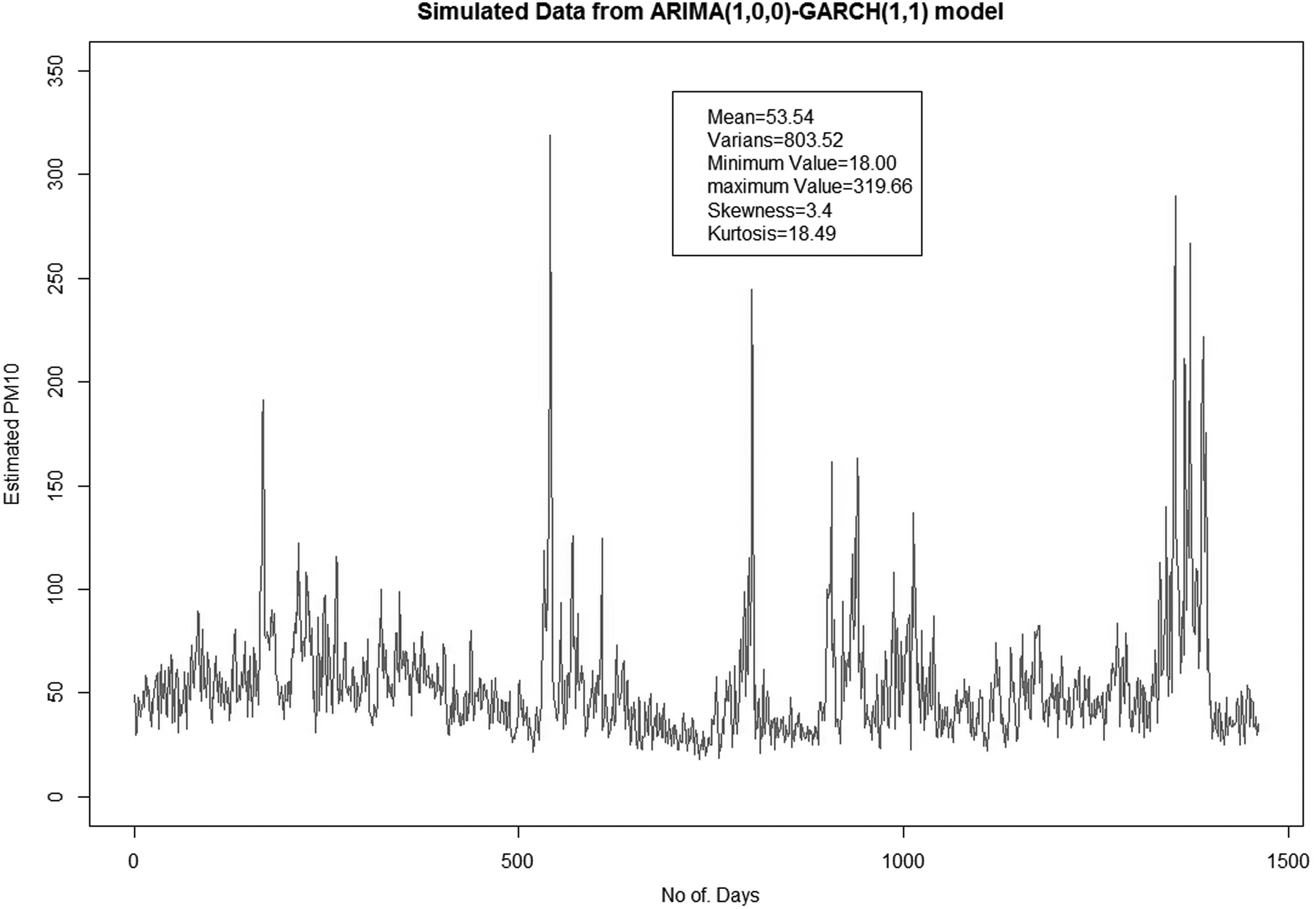
Next, using Equation (22), sample data from the ARMA(1,0)-GARCH(1,1) model can be simulated as shown in Fig. 9. The simulated data are relatively similar to the observational data in Fig. 1. Based on Fig. 9, it is found that all of the statistical measures obtained in the simulated data, such as the mean, variance, and so on, provide a very good similarity with the statistical measures from the original data, which are shown in Fig. 1.

FIG. 9.

Simulated data from ARMA(1,0)-GARCH(1,1) model.

Apart from that, we found that the value of R² coefficient for the single ARMA(1,0) model is 0.6269, which indicates that the ARMA(1,0) model is only able to describe ∼62.69% of the fluctuation in PM₁₀ data. However, after considering the effect of the volatility in the data presented by the ARMA(1,0)-GARCH(1,1) model, the value of R² increased to 0.93572, which implies that more than 90% of the PM₁₀ data can be described by the combination of the ARMA and GARCH models.

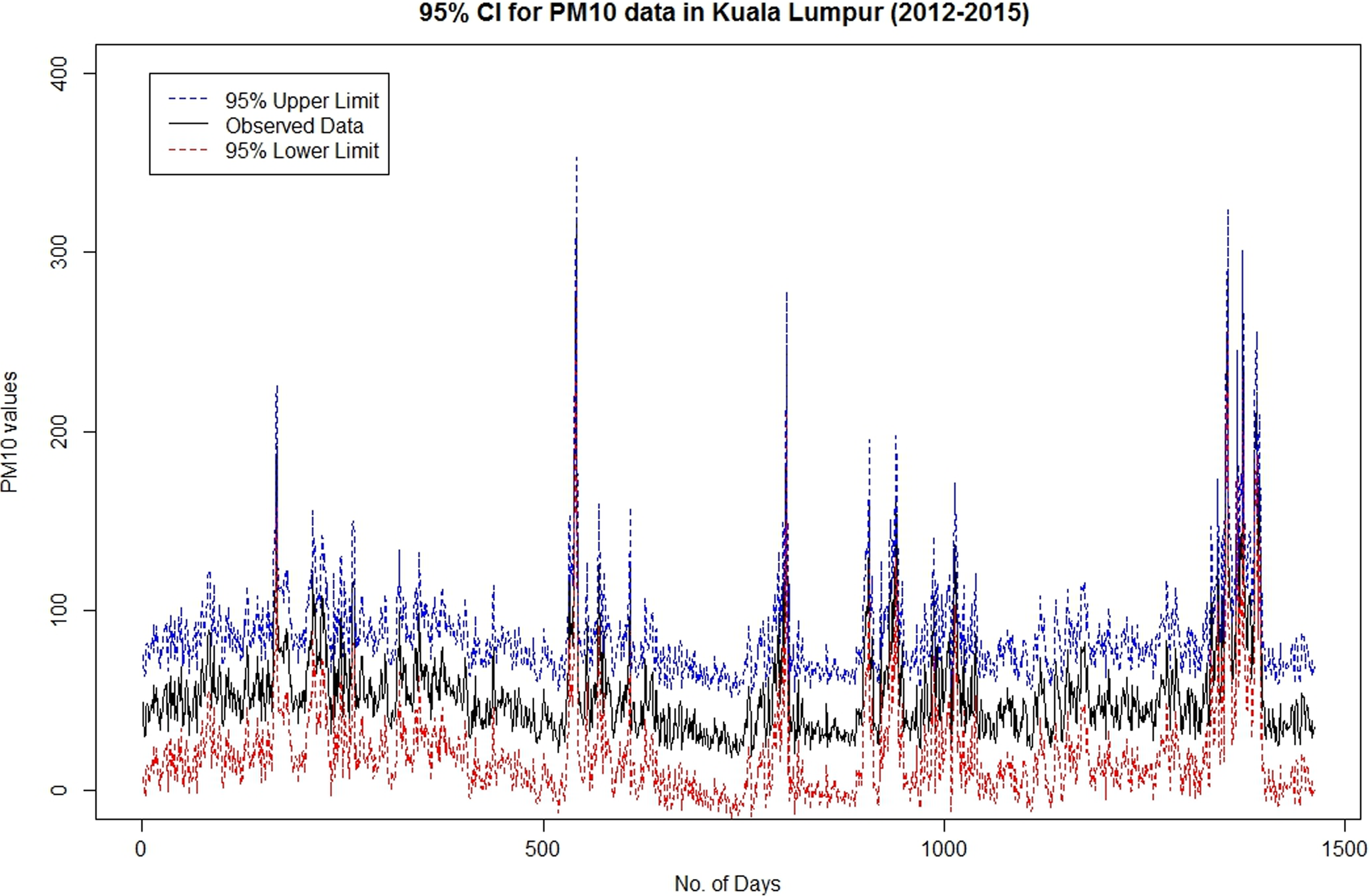
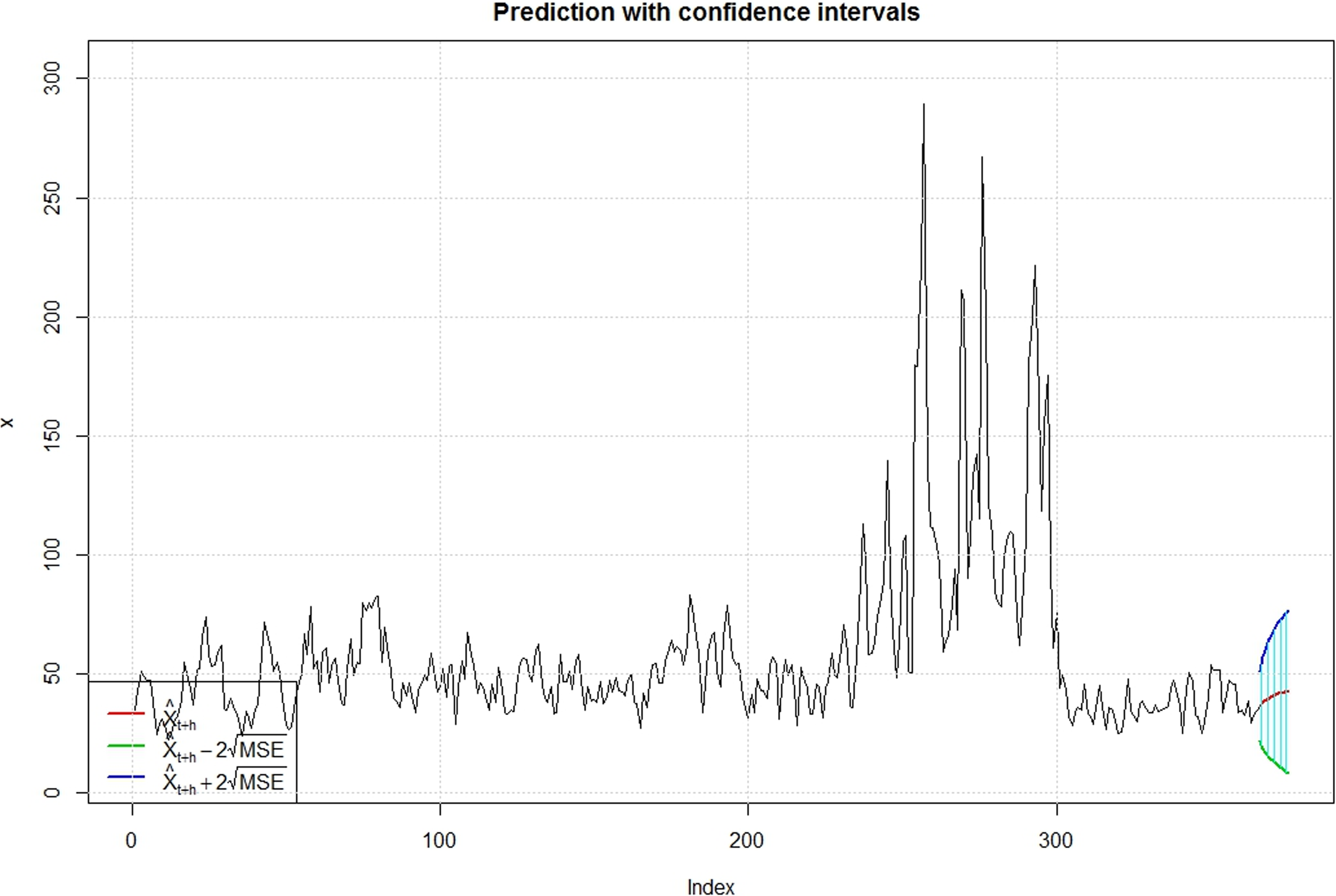
In addition, Fig. 10 shows the 95% confidence interval of the model for the original data set, while Fig. 11 and Table 3 show the 10-h prediction values for PM₁₀ in Kuala Lumpur, which are derived from the model. Based on the forecast value and its confidence interval, we believe that the values of PM₁₀ for the next 10 h will be in the average range of 36–42, with the lowest confidence interval being 8 and the highest interval being 76. These forecast values can be a good basis information to the public authorities to monitor the risk of recurrence in extreme air pollution. However, for a large future time horizon, the confidence interval of the forecasting will be larger. This implies that the accuracy of forecasting will be decreased. To provide a better assessment, this model needs to be reestimated to obtain a latest forecasting evaluation of PM₁₀ values over time. Thus, to use this model for air pollution forecasting and decision-making, the ARMA-GARCH model needs to be run every day to forecast the next 10-h of PM₁₀ data. Overall, we can conclude that the ARMA(1,0)-GARCH(1,1) is a good model to use when describing the fluctuation of the PM₁₀ data, which indicates the existence of a volatility effect.

FIG. 10.

Ninety-five confidence interval of model for original data set.

FIG. 11.

Prediction values with confidence intervals.

Table 3.

10-h Prediction Values for PM₁₀ in Kuala Lumpur

No. of prediction	Mean forecast	Mean error	Standard deviation	Lower interval	Upper interval
1	36.56287	7.306343	7.306343	21.950189	51.17556
2	37.97065	9.712417	7.785100	18.545819	57.39549
3	39.08957	11.292327	8.241673	16.504918	61.67423
4	39.97890	12.485662	8.679633	15.007581	64.95023
5	40.68576	13.465607	9.101732	13.754543	67.61697
6	41.24757	14.317445	9.510145	12.612682	69.88246
7	41.69411	15.087695	9.906628	11.518720	71.86950
8	42.04902	15.803273	10.292619	10.442478	73.65557
9	42.33111	16.480412	10.669315	9.370289	75.29194
10	42.55532	17.129245	11.037728	8.296832	76.81381

Conclusion

In this study, we proposed the method of ARMA with a combination of ARCH/GARCH approach to model the fluctuation of PM₁₀ data that exhibits an existence of the volatility effect. Based on the ACF and PACF graphs, the ARMA(1,0) model was determined to be a good approximation of the fluctuation in PM₁₀ data. However, the volatility effect has lowered the accuracy of the ARMA model. Thus, the analysis of the volatility effect in the residuals of the ARMA model was completed, based on the AIC values, which indicated that the GARCH(1,1) model was a good model to cover the volatility effect. Simulated data for ARMA(1,0)-GARCH(1,1) model was found to provide statistical properties similar to the original data. Apart from that, a confidence interval and the prediction values based on ARMA(1,0)-GARCH(1,1) have also been provided. However, to provide a better assessment, this model needs to be reestimated to obtain a latest forecasting evaluation of PM₁₀ values over time. The ARMA(1,0)-GARCH(1,1) model may be used as an operational tool for air quality forecasting in Kuala Lumpur or, with suitable adaptations, in any other large city in Malaysia. For further analysis, it is recommended that the volatility analysis regarding the fluctuation of PM₁₀ data involves a Markov Chain model or state space model. This is because once the volatility is occurring during the pollution events, it has a tendency to be influenced by the changes of the state/level of the data. Thus, it will be an interesting topic to be investigated.

Footnotes

Acknowledgments

The authors are indebted to the Department of Environment Malaysia for providing the air pollution data that made this article possible. This research would not be possible without the sponsorship from Universiti Kebangsaan Malaysia and Ministry of Higher Education in Malaysia (grant number FRGS/1/2014/SG04/UKM/03/1 and GP-K020446). In addition, the authors also thank all the anonymous reviewers for their critical comments and views that led to the improvement of this article.

Author Disclosure Statement

No competing financial interests exist.

References

Afroz

, Hassan

M.N.

, and Ibrahim

N.A.

(2003). Review of air pollution and health impact in Malaysia. Environ. Res., 92, 71.

Bell

M.L.

, Samet

J.M.

, and Dominici

(2004). Time-series studies of particulate matter. Annu. Rev. Public Health, 25, 247.

Bowerman

B.L.

, O'Connell

R.T.

, and Koehler

A.B

. (2005). Forecasting, Time Series and Regression, an Applied Approach, 4th edition. Belmont, CA: Thomson Brooks/Cole.

Chow

J.C.

, Bachmann

J.D.

, Wierman

S.S.G.

, Mathai

C.V.

, Malm

W.C.

, White

W.H.

, Mueller

P.K.

, Kumar

, and Watson

J.G.

(2002). Visibility: Science and regulation-discussion. J. Air Waste Manage. Assoc., 52, 973.

Cryer

J.D.

, and Chan

K.-S.

(2008). Time Series analysis: With Applications in R. New York: Springer.

Danielsson

(2011). Financial Risk Forecasting: The Theory and Practice of Forecasting Market Risk, with the Implementation in R and MATLAB. Wiltshire, United Kingdom: John Wiley & Sons.

Diaz-Robles

L.A.

, Ortega

J.C.

, Fu

J.S.

, Reed

G.D.

, Chow

J.C.

, Watson

J.G.

, and Moncada-Herrera

J.A.

(2008). A hybrid ARIMA and artificial neural network model to forecast particulate matter in urban areas: The case of Temuco, Chile. Atmos. Environ., 42, 8331.

Goldberg

M.S.

, Burnett

R.T.

, and Stieb

(2003). A review of time-series studies used to evaluate the short-term effects of air pollution on human health. Rev. Environ. Health, 18, 269.

Goyal

, Chan

A.T.

, and Jaiswal

(2006). Statistical models for the prediction of respirable suspended particulate matter in urban cities. Atmos. Environ., 40, 2068.

10.

Hirotugu

(1974). A new look at the statistical model identification. IEEE Trans. Automat. Control, 19, 716.

11.

Hooyberghs

, Mensink

, Dumont

, Fierens

, and Brasseur

(2005). A neural network forecast for daily average PM₁₀ concentrations in Belgium. Atmos. Environ., 39, 3279.

12.

Kumar

, and Ridder

K.D.

(2010). GARCH modelling in association with FFT-ARIMA to forecast ozone episodes. Atmos. Environ., 44, 4252.

13.

Masseran

(2016). Modeling the fluctuations of wind speed data by considering their mean and volatility effects. Renew. Sust. Energ. Rev., 54, 777.

14.

Masseran

, Razali

A.M.

, Ibrahim

, and Latif

M.T.

(2016). Modeling air quality in main cities of Peninsular Malaysia by using a generalized Pareto model. Environ. Monit. Assess., 188, Article number 65.

15.

Masseran

, Razali

A.M.

, Ibrahim

, Zaharim

, and Sopian

(2013a). Application of the single imputation method to estimate missing wind speed data in Malaysia. Res. J. Appl. Sci. Eng. Technol., 6, 1780.

16.

Masseran

, Razali

A.M.

, Ibrahim

, Zaharim

, and Sopian

(2013b). The probability distribution model of wind speed over East Malaysia. Res. J. Appl. Sci. Eng. Technol., 6, 1774.

17.

Milionis

A.E.

, and Davies

T.D.

(1994). Regression and stochastic models for air pollution-I, review, comments and suggestions. Atmos. Environ., 28, 2801.

18.

Peng

R.D.

, Dominici

, and Louis

T.A.

(2006). Model choice in time series studies of air pollution and mortality. J. R. Statist. Soc. A, 169, 179.

19.

Perez

, and Reyes

(2006). An integrated neural network model for PM10 forecasting. Atmos. Environ., 40, 2845.

20.

Poggi

J.-M.

, and Portier

(2011). PM10 forecasting using clusterwise regression. Atmos. Environ., 45, 7005.

21.

Pope

C.A.

, and Dockery

D.W.

(2006). Health effects of fine particulate air pollution: Lines that connect. J. Air Waste Manage. Assoc., 56, 709.

22.

Reisen

V.A.

, et al. (2014). Modeling and forecasting daily average PM10 concentrations by a seasonal long-memory model with volatility. Environ. Model. Softw., 51, 286.

23.

Sanhueza

, Vargas

, and Mellado

(2005). Impact of air pollution by fine particulate matter (PM10) on daily mortality in Temuco, Chile. Revista. Medica. De. Chile., 134, 754.

24.

Schlink

, Herbarth

, and Tetzlaff

(1997). A component time-series model for SO2 data: Forecasting, interpretation and modification. Atmos. Environ., 31, 1285.

25.

Shi

J.P.

, and Harrison

R.M.

(1997). Regression modeling of hourly NO_x and NO₂ concentrations in urban air in London. Atmos. Environ., 31, 4081.

26.

The World According to GaWC 2008. (2009). Globalization and World Cities Study Group and Network (GaWC). Loughborough University. Available at: www.lboro.ac.uk/gawc/world2008t.html Last accessed July 19, 2017.

27.

Tiwari

, Chate

D.M.

, Srivastava

A.K.

, Bisht

D.S.

, and Padmanabhamurty

(2012). Assessments of PM₁, PM_2.5 and PM₁₀ concentrations in Delhi at different mean cycles. Geofizika, 29, 125.

28.

Tsay

R.S.

(2005). Analysis of Financial Time Series, 2nd edition. NJ: John Wiley & Sons.

29.

Wei

W.W.S.

(2006). Time Series Analysis: Univariate and Multivariate Methods, 2nd edition. Boston, MA: Pearson Education.

30.

Wurtz

, Chalabi

, and Luksan

Parameter estimation of ARMA models with GARCH/APARCH errors. An R and SPlus software implementations. J. Stat. Softw. Available at: www-stat.wharton.upenn.edu/∼steele/Courses/956/RResources/GarchAndR/WurtzEtAlGarch.pdf Last accessed July 19, 2017.

Modeling Fluctuation of PM 10 Data with Existence of Volatility Effect

Abstract

Abstract

Introduction

Study Areas and Data

Modeling Fluctuations of PM10 Data

Single ARMA model

Single ARCH/GARCH model

ARMA model with ARCH/GARCH residual

Results and Discussion

Parameter estimation for the ARCH/GARCH model

Comparison of ARMA, GARCH, and ARMA-GARCH model

Conclusion

Footnotes

Acknowledgments

Author Disclosure Statement

References

Modeling Fluctuations of PM₁₀ Data