Water-related investments have been designed to contribute to economic development and public welfare. This study primarily aimed to perform a cost–benefit analysis on maintaining the sustainable development of water resources and improving the level for water pollution treatment in a transboundary river basin. This work systematically examined the organic connections of economic growth, wastewater discharge, and investment in environmental treatment. An integrated predictive model of transboundary river basin's treatment cost (TRBTC) was proposed to analyze the temporal–spatial dynamic changes in transboundary wastewater production and discharge, and modifications in treatment investment costs. The Songhua River Basin (SRB) was selected as the study area, and an integrated model of TRBTC was utilized to conduct temporal–spatial simulation, and analysis of wastewater treatment and discharge costs in the transboundary river basin during China's 13th Five-Year Plan. Results indicated that operational costs and investment costs of wastewater treatment in the SRB present an overall increasing tendency during the 13th Five-Year Plan. Respective operational and investment costs were 41.53% and 37.97% more than the costs during the 12th Five-Year Plan. With the continuous increase in treatment investment costs, total water pollutant discharge in the SRB has been controlled and water quality has been improved. This study offers practical relevance and provides a reference for management of investment and operation costs in water pollution control for further research and practical applications.
Introduction
The environment has been increasingly contaminated. For example, water pollution is the most comprehensive global environmental issue (Djukic et al., 2016). Water pollution control is not only a policy but also an economically technical problem. Water resource pollution and environmental protection have been recognized as serious issues (Malakoff, 2011; Degefu et al., 2016). Public attention has mainly focused on the cost-effectiveness of water pollution treatment in river basins to contribute to economic development and public welfare, especially in transboundary river basins. Decades ago, foreign scholars investigated the relationship of pollutant discharge, economic growth, and treatment investment (Hernandez-Sancho et al., 2011; Dore et al., 2012; Heather et al., 2013; Rinaudo and Aulong, 2014; Malm et al., 2015; Marzouk and Elkadi, 2016).
In 1955, Hammond, an American economist, applied the principles of cost–benefit analysis to the field of pollution control for the first time by evaluating the costs and benefits of water pollution control (Hernandez-Sancho et al., 2011; Kucukmehmetoglu, 2012; Ge et al., 2013; Ahn and Kang, 2014; Chetty and Pillay, 2015; Ruiz-Rosa et al., 2016). The United States, the United Kingdom, Canada, Japan, and other countries have also facilitated studies and applications regarding the cost–benefit analysis of environmental pollution control (Rodriguezgarcia et al., 2011; Pérez et al., 2012; Fatma et al., 2013; Hautakangas et al., 2014; Kurt et al., 2015; Atab et al., 2016). Studies on environmental protection and treatment investment in some developed European and American countries have been widely conducted (Molinos-Senante et al., 2011; Rocher et al., 2012; Jorsaraei et al., 2013; Shih and Tseng, 2014; Lange et al., 2015; Djukic et al., 2016).
For example, the US, Europe, and Australia have provided valuable experiences on the successful treatment of water pollution issues in transboundary river basins. The relationship between environmental pollution and economic growth has emerged as an important research topic in the field of environmental economics. Foreign countries have adopted cost–benefit analysis guaranteed by legislation as an important tool of environmental decision-making and have widely applied this tool in relevant environmental decision-making and major projects (Mohammad et al., 2011; Logar et al., 2014; Kearns et al., 2015; Eggimann et al., 2016; Moreno et al., 2016).
Studies on environmental economics in China began relatively late (Zhao et al., 2012; Wang et al., 2013; Li et al., 2016; Yu et al., 2016a). With the implementation of environmental protection and treatment measures, the importance of environmental cost–benefit analysis has been acknowledged. Domestic scholars utilized various techniques, including Computable General Equilibrium modeling, systematic dynamic (SD) method, and optimized decision-making modeling, to investigate treatment investments in the environmental field (Liu et al., 2014; Yu et al., 2015a; Zhou et al., 2015; Niu et al., 2016). Studies on the treatment costs of water pollution in transboundary river basins are considered not only a policy issue but also an economic and technological concern because of several interests of different stakeholders, numerous aspects, and highly complex transboundary regions.
Therefore, the comprehensive utilization of relevant technological methods, such as economics, environmental science, and statistics, to carry out studies on investment costs and operational costs of water pollution control in transboundary river basins has become urgent. However, insufficient studies have been performed regarding the estimation of transboundary river basin's treatment cost (TRBTC), and an integrated model should be developed to conduct this estimation. In particular, policy makers face challenges on how to balance the tradeoff between the overall goal of total mass control for environmental quality protection and the economic benefit of different regions influenced by the allocation of wastewater production and discharge in a transboundary river basin. Thus, the lack of such considerations can hardly guarantee the generation of an economically and environmentally harmonious development at a watershed level. Water pollution and its treatment in transboundary river basins have remained as urgent, unresolved, and difficult problems.
To develop efficient instruments and policies related to water quality and water management, we should obtain insights into the overall value of water resources that should be measured and incorporated in policy decision administration. With the assessment of water pollution treatment costs, water resource agencies have been regulated in terms of the use of high-quality water and recycled water for industrial and agricultural purposes to utilize limited resources, such as money, and to improve the efficiency of river basin pollution control and governance, especially those related to cost recovery for water services. Economic valuation is presented as a useful tool to implement efficient and effective policies and strategies for the management of transboundary river basins.
Comprehensive Predictive Model of TRBTC
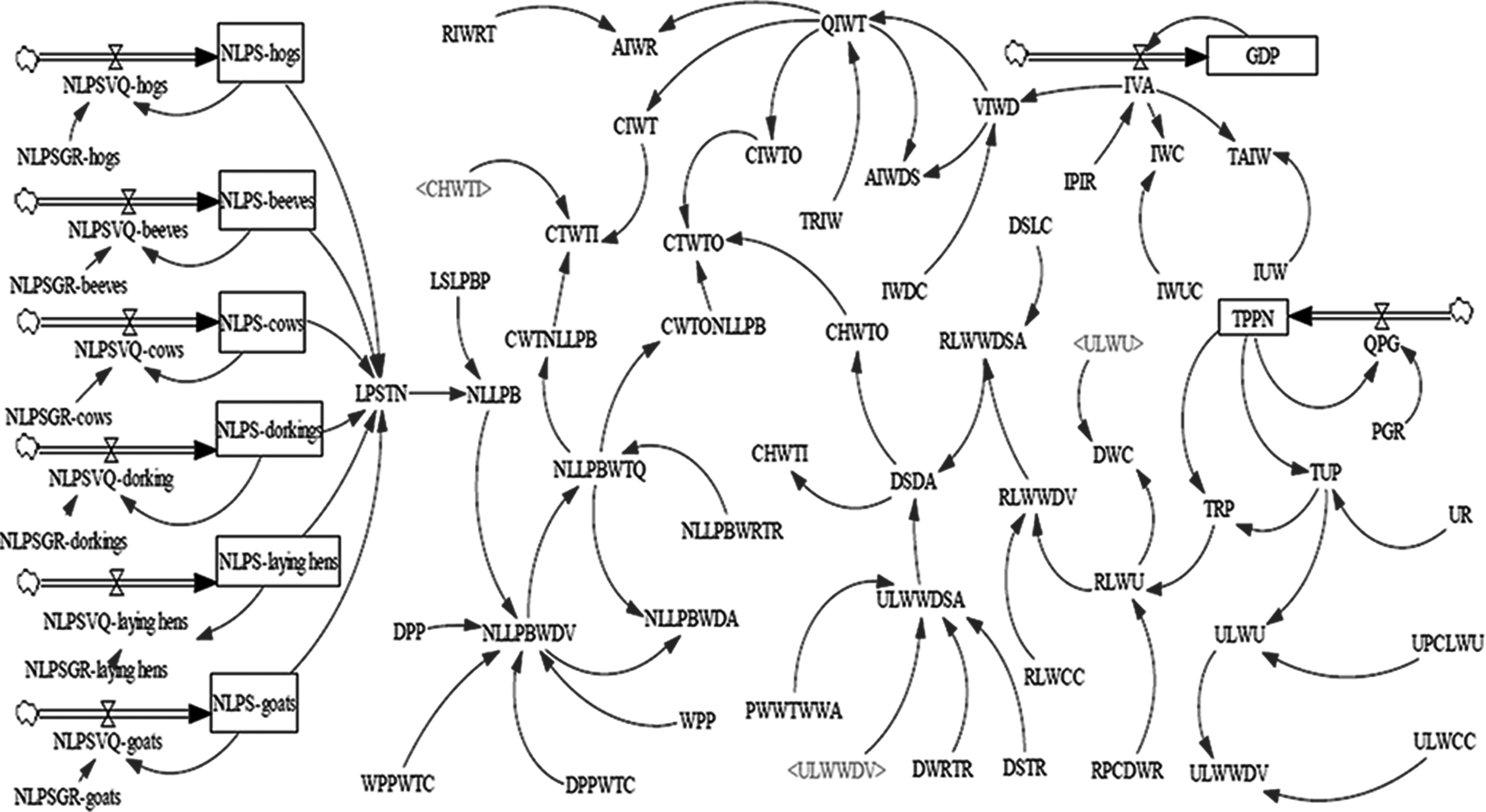
Considering perspectives on the sustainable development of water resources, namely, industry, livestock and poultry breeding, and urban and rural households, we investigated the underlying mechanism to reveal the combined control of water resources, water pollution, and treatment cost in the Songhua River Basin (SRB). A coupling relationship was established among water resources, water environment, and economy in the SRB. The framework of the TRBTC model was designed by comprehensively considering the economic and social development strategic arrangement, and the water resource and aquatic environmental pollution treatment planning of transboundary river basins. Furthermore, the temporal–spatial characteristics were identified and analyzed in terms of water resource consumption, wastewater treatment procedures, investment on water pollution treatment during China's 12th Five-year plan, and other parameters. We screened the typical indicators according to the temporal–spatial characteristics. An SD method was applied to establish the relationship between social economy, wastewater production and discharge, and investment and operational costs of water pollution treatment in transboundary river basins. Figure 1 describes the organic connection and interior relationships, and Supplementary Table S1 defines the corresponding parameters and variables.
\documentclass{aastex}\usepackage{amsbsy}\usepackage{amsfonts}\usepackage{amssymb}\usepackage{bm}\usepackage{mathrsfs}\usepackage{pifont}\usepackage{stmaryrd}\usepackage{textcomp}\usepackage{portland, xspace}\usepackage{amsmath, amsxtra}\usepackage{upgreek}\pagestyle{empty}\DeclareMathSizes{10}{9}{7}{6}\begin{document}
\begin{align*}
{C_{total}} = {C_{total \_ \, I}} + {C_{total \_ \, R}} \\
= \mathop \sum_{t = 1}^T \mathop \sum_{g = 1}^G \left\{ {C_{I \_
\, I}} ( Q , \mu , \phi , \kappa , \pi , g , t )
, \right. \\
\left.C_{LC \_ \, I} ( P , \gamma , \eta , \xi , \tau , \upsilon ,
g , t ) , {C_{LS \_ \, I}} \ ( P , \lambda
, \alpha , \delta , \beta , \varepsilon , g , t ) \right\} \\
+ \sum \limits_{t = 1}^T \sum \limits_{g = 1}^G
\{ {C_{I \_ \, R}} ( Q , \omega , \sigma , \psi , g , t ) ,\\
{C_{LC \_ \, R}}\ ( P , \gamma , \chi , \theta , g , t ) , {C_{LS
\_}}{_R} ( P , \lambda , \alpha , \delta , \beta , o , g , t ) \}
\tag{1}
\end{align*}
\end{document}
Dynamic coupling relationship of wastewater discharge and treatment costs.
Equation (1) generally represents the total costs of wastewater treatment (\documentclass{aastex}\usepackage{amsbsy}\usepackage{amsfonts}\usepackage{amssymb}\usepackage{bm}\usepackage{mathrsfs}\usepackage{pifont}\usepackage{stmaryrd}\usepackage{textcomp}\usepackage{portland, xspace}\usepackage{amsmath, amsxtra}\usepackage{upgreek}\pagestyle{empty}\DeclareMathSizes{10}{9}{7}{6}\begin{document}
$${C_{total}}$$
\end{document}), including wastewater discharge treatment investment costs (\documentclass{aastex}\usepackage{amsbsy}\usepackage{amsfonts}\usepackage{amssymb}\usepackage{bm}\usepackage{mathrsfs}\usepackage{pifont}\usepackage{stmaryrd}\usepackage{textcomp}\usepackage{portland, xspace}\usepackage{amsmath, amsxtra}\usepackage{upgreek}\pagestyle{empty}\DeclareMathSizes{10}{9}{7}{6}\begin{document}
$${C_{total \_ \, I}}$$
\end{document}) and wastewater discharge treatment operational costs (\documentclass{aastex}\usepackage{amsbsy}\usepackage{amsfonts}\usepackage{amssymb}\usepackage{bm}\usepackage{mathrsfs}\usepackage{pifont}\usepackage{stmaryrd}\usepackage{textcomp}\usepackage{portland, xspace}\usepackage{amsmath, amsxtra}\usepackage{upgreek}\pagestyle{empty}\DeclareMathSizes{10}{9}{7}{6}\begin{document}
$${C_{total \_ \, R}}$$
\end{document}). The definitions of several symbols in this equation are explained in the following sections. Wastewater discharge treatment investment costs (\documentclass{aastex}\usepackage{amsbsy}\usepackage{amsfonts}\usepackage{amssymb}\usepackage{bm}\usepackage{mathrsfs}\usepackage{pifont}\usepackage{stmaryrd}\usepackage{textcomp}\usepackage{portland, xspace}\usepackage{amsmath, amsxtra}\usepackage{upgreek}\pagestyle{empty}\DeclareMathSizes{10}{9}{7}{6}\begin{document}
$${C_{total \_ \, I}}$$
\end{document}) include industrial wastewater discharge treatment investment costs (\documentclass{aastex}\usepackage{amsbsy}\usepackage{amsfonts}\usepackage{amssymb}\usepackage{bm}\usepackage{mathrsfs}\usepackage{pifont}\usepackage{stmaryrd}\usepackage{textcomp}\usepackage{portland, xspace}\usepackage{amsmath, amsxtra}\usepackage{upgreek}\pagestyle{empty}\DeclareMathSizes{10}{9}{7}{6}\begin{document}
$${C_{I \_ \, I}}$$
\end{document}), household wastewater discharge treatment investment costs (\documentclass{aastex}\usepackage{amsbsy}\usepackage{amsfonts}\usepackage{amssymb}\usepackage{bm}\usepackage{mathrsfs}\usepackage{pifont}\usepackage{stmaryrd}\usepackage{textcomp}\usepackage{portland, xspace}\usepackage{amsmath, amsxtra}\usepackage{upgreek}\pagestyle{empty}\DeclareMathSizes{10}{9}{7}{6}\begin{document}
$${C_{LC \_ \, I}}$$
\end{document}), and wastewater discharge treatment investment costs of raising livestock and poultry (\documentclass{aastex}\usepackage{amsbsy}\usepackage{amsfonts}\usepackage{amssymb}\usepackage{bm}\usepackage{mathrsfs}\usepackage{pifont}\usepackage{stmaryrd}\usepackage{textcomp}\usepackage{portland, xspace}\usepackage{amsmath, amsxtra}\usepackage{upgreek}\pagestyle{empty}\DeclareMathSizes{10}{9}{7}{6}\begin{document}
$${C_{LS \_ \, I}}$$
\end{document}). Wastewater discharge treatment operational costs (\documentclass{aastex}\usepackage{amsbsy}\usepackage{amsfonts}\usepackage{amssymb}\usepackage{bm}\usepackage{mathrsfs}\usepackage{pifont}\usepackage{stmaryrd}\usepackage{textcomp}\usepackage{portland, xspace}\usepackage{amsmath, amsxtra}\usepackage{upgreek}\pagestyle{empty}\DeclareMathSizes{10}{9}{7}{6}\begin{document}
$${C_{total \_ \, R}}$$
\end{document}) cover industrial wastewater discharge treatment operational costs (\documentclass{aastex}\usepackage{amsbsy}\usepackage{amsfonts}\usepackage{amssymb}\usepackage{bm}\usepackage{mathrsfs}\usepackage{pifont}\usepackage{stmaryrd}\usepackage{textcomp}\usepackage{portland, xspace}\usepackage{amsmath, amsxtra}\usepackage{upgreek}\pagestyle{empty}\DeclareMathSizes{10}{9}{7}{6}\begin{document}
$${C_{I \_ \, R}}$$
\end{document}), household wastewater discharge treatment operational costs (\documentclass{aastex}\usepackage{amsbsy}\usepackage{amsfonts}\usepackage{amssymb}\usepackage{bm}\usepackage{mathrsfs}\usepackage{pifont}\usepackage{stmaryrd}\usepackage{textcomp}\usepackage{portland, xspace}\usepackage{amsmath, amsxtra}\usepackage{upgreek}\pagestyle{empty}\DeclareMathSizes{10}{9}{7}{6}\begin{document}
$${C_{LC \_ \, R}}$$
\end{document}), and wastewater discharge treatment operational costs of raising livestock and poultry (\documentclass{aastex}\usepackage{amsbsy}\usepackage{amsfonts}\usepackage{amssymb}\usepackage{bm}\usepackage{mathrsfs}\usepackage{pifont}\usepackage{stmaryrd}\usepackage{textcomp}\usepackage{portland, xspace}\usepackage{amsmath, amsxtra}\usepackage{upgreek}\pagestyle{empty}\DeclareMathSizes{10}{9}{7}{6}\begin{document}
$${C_{LS \_ \, R}}$$
\end{document}). T denotes the year and G refers to the grid units dividing the river basin.
Calculation of industrial wastewater discharge treatment costs
Equation (2) represents the industrial wastewater discharge treatment investment costs (\documentclass{aastex}\usepackage{amsbsy}\usepackage{amsfonts}\usepackage{amssymb}\usepackage{bm}\usepackage{mathrsfs}\usepackage{pifont}\usepackage{stmaryrd}\usepackage{textcomp}\usepackage{portland, xspace}\usepackage{amsmath, amsxtra}\usepackage{upgreek}\pagestyle{empty}\DeclareMathSizes{10}{9}{7}{6}\begin{document}
$${C_{I \_ \, I}}$$
\end{document}), and Equation (3) describes the industrial wastewater discharge treatment operational costs (\documentclass{aastex}\usepackage{amsbsy}\usepackage{amsfonts}\usepackage{amssymb}\usepackage{bm}\usepackage{mathrsfs}\usepackage{pifont}\usepackage{stmaryrd}\usepackage{textcomp}\usepackage{portland, xspace}\usepackage{amsmath, amsxtra}\usepackage{upgreek}\pagestyle{empty}\DeclareMathSizes{10}{9}{7}{6}\begin{document}
$${C_{I \_ \, R}}$$
\end{document}). The key input parameters in Equations (2)and (3) are listed in Supplementary Table S2. We determined the relationship between industrial wastewater treatment investment and wastewater discharge and then established a model of the investment and operational costs of industrial wastewater treatment through a comprehensive analysis of the systematic process characteristics of industrial wastewater production and discharge, wastewater treatment procedures, and wastewater treatment investment and operational costs in the transboundary river basin:
\documentclass{aastex}\usepackage{amsbsy}\usepackage{amsfonts}\usepackage{amssymb}\usepackage{bm}\usepackage{mathrsfs}\usepackage{pifont}\usepackage{stmaryrd}\usepackage{textcomp}\usepackage{portland, xspace}\usepackage{amsmath, amsxtra}\usepackage{upgreek}\pagestyle{empty}\DeclareMathSizes{10}{9}{7}{6}\begin{document}
\begin{align*}
\begin{split}
C_{I \_ \, I}= \mathop \sum \limits_{t = 1}^T \mathop \sum
\limits_{g = 1}^G \big( \mathop \sum \limits_{j = 1}^{39} \big(
\big[ {Q_{TID \_j \_ \,g \_\,t} \over {365 \times { \kappa _{j \_
\, g \_ \, t}} \times { \pi _{j \_ \, g \_ \,
t}}}} \\
+ {Q_{LID \_j \_ \,g \_\,t}} \times ( { \mu _{j \_ \, g \_ \, t}}
- 1 ) \big] \times { \phi _{j \_ \, g \_ \, t}} \big)
\big)\end{split}
\tag{2}
\end{align*}
\end{document}\documentclass{aastex}\usepackage{amsbsy}\usepackage{amsfonts}\usepackage{amssymb}\usepackage{bm}\usepackage{mathrsfs}\usepackage{pifont}\usepackage{stmaryrd}\usepackage{textcomp}\usepackage{portland, xspace}\usepackage{amsmath, amsxtra}\usepackage{upgreek}\pagestyle{empty}\DeclareMathSizes{10}{9}{7}{6}\begin{document}
\begin{align*}
{C_{I \_ \, R}} = \mathop \sum \limits_{t = 1}^T { \mathop \sum \limits_{g = 1}^G { \mathop \sum \limits_{j = 1}^{39} {{G_{IAV \_j \_ \,g \_ \,t}} \times { \omega _{j \_ \, g \_ \, t}} \times { \sigma _{j \_ \, g \_ \, t}} \times { \psi _{j \_ \, g \_ \, t}}} } } \tag{3}
\end{align*}
\end{document}
where \documentclass{aastex}\usepackage{amsbsy}\usepackage{amsfonts}\usepackage{amssymb}\usepackage{bm}\usepackage{mathrsfs}\usepackage{pifont}\usepackage{stmaryrd}\usepackage{textcomp}\usepackage{portland, xspace}\usepackage{amsmath, amsxtra}\usepackage{upgreek}\pagestyle{empty}\DeclareMathSizes{10}{9}{7}{6}\begin{document}
$${C_{I \_ \, I}}$$
\end{document} is the industrial wastewater treatment cost (unit, 0.1 billion CNY); \documentclass{aastex}\usepackage{amsbsy}\usepackage{amsfonts}\usepackage{amssymb}\usepackage{bm}\usepackage{mathrsfs}\usepackage{pifont}\usepackage{stmaryrd}\usepackage{textcomp}\usepackage{portland, xspace}\usepackage{amsmath, amsxtra}\usepackage{upgreek}\pagestyle{empty}\DeclareMathSizes{10}{9}{7}{6}\begin{document}
$${C_{I \_ \, R}}$$
\end{document} is the industrial wastewater treatment operational cost (unit, 0.1 billion CNY); j is the total number of industries (j = 1, 2, 3, …, 39); \documentclass{aastex}\usepackage{amsbsy}\usepackage{amsfonts}\usepackage{amssymb}\usepackage{bm}\usepackage{mathrsfs}\usepackage{pifont}\usepackage{stmaryrd}\usepackage{textcomp}\usepackage{portland, xspace}\usepackage{amsmath, amsxtra}\usepackage{upgreek}\pagestyle{empty}\DeclareMathSizes{10}{9}{7}{6}\begin{document}
$${Q_{NID \_j \_ \,g \_\,t}}$$
\end{document} is the current-year wastewater treatment quantity of the j_th industry in the g_th zone at the t_th time (unit, 10 thousand tons); \documentclass{aastex}\usepackage{amsbsy}\usepackage{amsfonts}\usepackage{amssymb}\usepackage{bm}\usepackage{mathrsfs}\usepackage{pifont}\usepackage{stmaryrd}\usepackage{textcomp}\usepackage{portland, xspace}\usepackage{amsmath, amsxtra}\usepackage{upgreek}\pagestyle{empty}\DeclareMathSizes{10}{9}{7}{6}\begin{document}
$${Q_{LID \_j \_ \,g \_\,t}}$$
\end{document} is the previous-year wastewater treatment quantity of the j_th industry in the g_th zone at the t_th time (unit, 10 thousand tons); \documentclass{aastex}\usepackage{amsbsy}\usepackage{amsfonts}\usepackage{amssymb}\usepackage{bm}\usepackage{mathrsfs}\usepackage{pifont}\usepackage{stmaryrd}\usepackage{textcomp}\usepackage{portland, xspace}\usepackage{amsmath, amsxtra}\usepackage{upgreek}\pagestyle{empty}\DeclareMathSizes{10}{9}{7}{6}\begin{document}
$${ \kappa _{j \_ \, g \_ \, t}}$$
\end{document} is the normal operating rate of the treatment equipment of the j_th industry in the g_th zone at the t_th time (unit, %); \documentclass{aastex}\usepackage{amsbsy}\usepackage{amsfonts}\usepackage{amssymb}\usepackage{bm}\usepackage{mathrsfs}\usepackage{pifont}\usepackage{stmaryrd}\usepackage{textcomp}\usepackage{portland, xspace}\usepackage{amsmath, amsxtra}\usepackage{upgreek}\pagestyle{empty}\DeclareMathSizes{10}{9}{7}{6}\begin{document}
$${ \pi _{j \_ \, g \_ \, t}}$$
\end{document} is the operating safety factor of the j_th industry in the g_th zone at the t_th time (unit, %); \documentclass{aastex}\usepackage{amsbsy}\usepackage{amsfonts}\usepackage{amssymb}\usepackage{bm}\usepackage{mathrsfs}\usepackage{pifont}\usepackage{stmaryrd}\usepackage{textcomp}\usepackage{portland, xspace}\usepackage{amsmath, amsxtra}\usepackage{upgreek}\pagestyle{empty}\DeclareMathSizes{10}{9}{7}{6}\begin{document}
$${ \mu _{j \_ \, g \_ \, t}}$$
\end{document} is the depreciation rate of equipment of the j_th industry in the g_th zone at the t_th time (unit, %); \documentclass{aastex}\usepackage{amsbsy}\usepackage{amsfonts}\usepackage{amssymb}\usepackage{bm}\usepackage{mathrsfs}\usepackage{pifont}\usepackage{stmaryrd}\usepackage{textcomp}\usepackage{portland, xspace}\usepackage{amsmath, amsxtra}\usepackage{upgreek}\pagestyle{empty}\DeclareMathSizes{10}{9}{7}{6}\begin{document}
$${ \phi _{j \_ \, g \_ \, t}}$$
\end{document} is the investment coefficient per unit of wastewater treatment of the j_th industry in the g_th zone at the t_th t ime (unit, CNY/ton); \documentclass{aastex}\usepackage{amsbsy}\usepackage{amsfonts}\usepackage{amssymb}\usepackage{bm}\usepackage{mathrsfs}\usepackage{pifont}\usepackage{stmaryrd}\usepackage{textcomp}\usepackage{portland, xspace}\usepackage{amsmath, amsxtra}\usepackage{upgreek}\pagestyle{empty}\DeclareMathSizes{10}{9}{7}{6}\begin{document}
$${G_{IAV \_j \_ \,g \_\,t}}$$
\end{document} is the industrial added value of the j_th industry in the g_th zone at the t_th time (unit, 10 thousand CNY); \documentclass{aastex}\usepackage{amsbsy}\usepackage{amsfonts}\usepackage{amssymb}\usepackage{bm}\usepackage{mathrsfs}\usepackage{pifont}\usepackage{stmaryrd}\usepackage{textcomp}\usepackage{portland, xspace}\usepackage{amsmath, amsxtra}\usepackage{upgreek}\pagestyle{empty}\DeclareMathSizes{10}{9}{7}{6}\begin{document}
$${ \omega _{j \_ \, g \_ \, t}}$$
\end{document} is the wastewater production coefficient of the j_th industry in the g_th zone at the t_th time (unit, ton/10,000 CNY); \documentclass{aastex}\usepackage{amsbsy}\usepackage{amsfonts}\usepackage{amssymb}\usepackage{bm}\usepackage{mathrsfs}\usepackage{pifont}\usepackage{stmaryrd}\usepackage{textcomp}\usepackage{portland, xspace}\usepackage{amsmath, amsxtra}\usepackage{upgreek}\pagestyle{empty}\DeclareMathSizes{10}{9}{7}{6}\begin{document}
$${ \sigma _{j \_ \, g \_ \, t}}$$
\end{document} is the wastewater treatment rate of the j_th industry in the g_th zone at the t_th time (unit, %); and \documentclass{aastex}\usepackage{amsbsy}\usepackage{amsfonts}\usepackage{amssymb}\usepackage{bm}\usepackage{mathrsfs}\usepackage{pifont}\usepackage{stmaryrd}\usepackage{textcomp}\usepackage{portland, xspace}\usepackage{amsmath, amsxtra}\usepackage{upgreek}\pagestyle{empty}\DeclareMathSizes{10}{9}{7}{6}\begin{document}
$${ \psi _{j \_ \, g \_ \, t}}$$
\end{document} is the operational coefficient of one unit of wastewater of the j_th industry in the g_th zone at the t_th time (unit, CNY/ton).
Calculation of household wastewater pollution treatment costs
Equation (4) represents the household wastewater discharge treatment investment costs (\documentclass{aastex}\usepackage{amsbsy}\usepackage{amsfonts}\usepackage{amssymb}\usepackage{bm}\usepackage{mathrsfs}\usepackage{pifont}\usepackage{stmaryrd}\usepackage{textcomp}\usepackage{portland, xspace}\usepackage{amsmath, amsxtra}\usepackage{upgreek}\pagestyle{empty}\DeclareMathSizes{10}{9}{7}{6}\begin{document}
$${C_{LC \_ \, I}}$$
\end{document}), and Equation (5) shows the household wastewater discharge treatment operational costs (\documentclass{aastex}\usepackage{amsbsy}\usepackage{amsfonts}\usepackage{amssymb}\usepackage{bm}\usepackage{mathrsfs}\usepackage{pifont}\usepackage{stmaryrd}\usepackage{textcomp}\usepackage{portland, xspace}\usepackage{amsmath, amsxtra}\usepackage{upgreek}\pagestyle{empty}\DeclareMathSizes{10}{9}{7}{6}\begin{document}
$${C_{LC \_ \, R}}$$
\end{document}). The key input parameters in Equations (4)and (5) are listed in Supplementary Table S3. The household wastewater treatment system in the transboundary river basin is complicated with many influencing factors. Parameters were selected according to the principles of comprehensiveness, priority, quantification, and controllability. The temporal–spatial distribution characteristics and the differences in household wastewater discharge were combined, and the relationship between water pollution treatment investment and household wastewater discharge was constructed. The model of the investment and operational costs of household wastewater treatment was established as follows:
\documentclass{aastex}\usepackage{amsbsy}\usepackage{amsfonts}\usepackage{amssymb}\usepackage{bm}\usepackage{mathrsfs}\usepackage{pifont}\usepackage{stmaryrd}\usepackage{textcomp}\usepackage{portland, xspace}\usepackage{amsmath, amsxtra}\usepackage{upgreek}\pagestyle{empty}\DeclareMathSizes{10}{9}{7}{6}\begin{document}
\begin{align*}
\begin{split}{C_{LC \_ \, I}} = \mathop \sum \limits_{t = 1}^T \mathop \sum \limits_{g = 1}^G ( {P_{U \_ \,g \_\,t}} \times {\gamma _{g \_t}} \times {\eta _{g \_t}} \times {\xi _{g \_t}} \\ \times {\tau ^2}_{g \_t} \times {\tau ^3}_{g \_t} \times {\upsilon _{g \_t}} \times 365 )\end{split}
\tag{4}
\end{align*}
\end{document}\documentclass{aastex}\usepackage{amsbsy}\usepackage{amsfonts}\usepackage{amssymb}\usepackage{bm}\usepackage{mathrsfs}\usepackage{pifont}\usepackage{stmaryrd}\usepackage{textcomp}\usepackage{portland, xspace}\usepackage{amsmath, amsxtra}\usepackage{upgreek}\pagestyle{empty}\DeclareMathSizes{10}{9}{7}{6}\begin{document}
\begin{align*}
{C_{LC \_ \, R}} = \mathop \sum \limits_{t = 1}^T { \mathop \sum \limits_{g = 1}^G ( } {P_{U \_ \,g \_\,t}} \times { \gamma _{g \_t}} \times { \chi _{g \_t}} \times { \theta _{g \_t}} ) \tag{5}
\end{align*}
\end{document}
where \documentclass{aastex}\usepackage{amsbsy}\usepackage{amsfonts}\usepackage{amssymb}\usepackage{bm}\usepackage{mathrsfs}\usepackage{pifont}\usepackage{stmaryrd}\usepackage{textcomp}\usepackage{portland, xspace}\usepackage{amsmath, amsxtra}\usepackage{upgreek}\pagestyle{empty}\DeclareMathSizes{10}{9}{7}{6}\begin{document}
$${C_{LC \_ \, I}}$$
\end{document} is the household wastewater treatment investment cost (unit, 0.1 billion CNY); \documentclass{aastex}\usepackage{amsbsy}\usepackage{amsfonts}\usepackage{amssymb}\usepackage{bm}\usepackage{mathrsfs}\usepackage{pifont}\usepackage{stmaryrd}\usepackage{textcomp}\usepackage{portland, xspace}\usepackage{amsmath, amsxtra}\usepackage{upgreek}\pagestyle{empty}\DeclareMathSizes{10}{9}{7}{6}\begin{document}
$${C_{LC \_ \, R}}$$
\end{document} is the household wastewater treatment operational cost (unit, 0.1 billion CNY); \documentclass{aastex}\usepackage{amsbsy}\usepackage{amsfonts}\usepackage{amssymb}\usepackage{bm}\usepackage{mathrsfs}\usepackage{pifont}\usepackage{stmaryrd}\usepackage{textcomp}\usepackage{portland, xspace}\usepackage{amsmath, amsxtra}\usepackage{upgreek}\pagestyle{empty}\DeclareMathSizes{10}{9}{7}{6}\begin{document}
$${P_{U \_ \,g \_\,t}}$$
\end{document} is the size of the urban population in the g_th zone at the t_th time (unit, 104 Person); \documentclass{aastex}\usepackage{amsbsy}\usepackage{amsfonts}\usepackage{amssymb}\usepackage{bm}\usepackage{mathrsfs}\usepackage{pifont}\usepackage{stmaryrd}\usepackage{textcomp}\usepackage{portland, xspace}\usepackage{amsmath, amsxtra}\usepackage{upgreek}\pagestyle{empty}\DeclareMathSizes{10}{9}{7}{6}\begin{document}
$${ \gamma _{g \_t}}$$
\end{document} is the urban household wastewater production coefficient per capita in the g_th zone at the t_th time (unit, L/person.d); \documentclass{aastex}\usepackage{amsbsy}\usepackage{amsfonts}\usepackage{amssymb}\usepackage{bm}\usepackage{mathrsfs}\usepackage{pifont}\usepackage{stmaryrd}\usepackage{textcomp}\usepackage{portland, xspace}\usepackage{amsmath, amsxtra}\usepackage{upgreek}\pagestyle{empty}\DeclareMathSizes{10}{9}{7}{6}\begin{document}
$${ \xi _{g \_t}}$$
\end{document} is the household water consumption percentage in the g_th zone at the t_th time (unit, %); \documentclass{aastex}\usepackage{amsbsy}\usepackage{amsfonts}\usepackage{amssymb}\usepackage{bm}\usepackage{mathrsfs}\usepackage{pifont}\usepackage{stmaryrd}\usepackage{textcomp}\usepackage{portland, xspace}\usepackage{amsmath, amsxtra}\usepackage{upgreek}\pagestyle{empty}\DeclareMathSizes{10}{9}{7}{6}\begin{document}
$${ \chi _{_{g \_t}}}$$
\end{document} is the urban household wastewater treatment rate in the g_th zone at the t_th time (unit, %); \documentclass{aastex}\usepackage{amsbsy}\usepackage{amsfonts}\usepackage{amssymb}\usepackage{bm}\usepackage{mathrsfs}\usepackage{pifont}\usepackage{stmaryrd}\usepackage{textcomp}\usepackage{portland, xspace}\usepackage{amsmath, amsxtra}\usepackage{upgreek}\pagestyle{empty}\DeclareMathSizes{10}{9}{7}{6}\begin{document}
$${ \theta _{g \_t}}$$
\end{document} is the operational coefficient per unit of wastewater in the g_th zone at the t_th time (unit, CNY/kg); \documentclass{aastex}\usepackage{amsbsy}\usepackage{amsfonts}\usepackage{amssymb}\usepackage{bm}\usepackage{mathrsfs}\usepackage{pifont}\usepackage{stmaryrd}\usepackage{textcomp}\usepackage{portland, xspace}\usepackage{amsmath, amsxtra}\usepackage{upgreek}\pagestyle{empty}\DeclareMathSizes{10}{9}{7}{6}\begin{document}
$${ \eta _{g \_t}}$$
\end{document} is the normal operating rate of treatment equipment in the g_th zone at the t_th time (unit, %); \documentclass{aastex}\usepackage{amsbsy}\usepackage{amsfonts}\usepackage{amssymb}\usepackage{bm}\usepackage{mathrsfs}\usepackage{pifont}\usepackage{stmaryrd}\usepackage{textcomp}\usepackage{portland, xspace}\usepackage{amsmath, amsxtra}\usepackage{upgreek}\pagestyle{empty}\DeclareMathSizes{10}{9}{7}{6}\begin{document}
$${ \tau ^2}_{g \_t}$$
\end{document} is the percentage of urban secondary wastewater treatment capacity of municipal wastewater treatment facilities in the g_th zone at the t_th time (unit, %); \documentclass{aastex}\usepackage{amsbsy}\usepackage{amsfonts}\usepackage{amssymb}\usepackage{bm}\usepackage{mathrsfs}\usepackage{pifont}\usepackage{stmaryrd}\usepackage{textcomp}\usepackage{portland, xspace}\usepackage{amsmath, amsxtra}\usepackage{upgreek}\pagestyle{empty}\DeclareMathSizes{10}{9}{7}{6}\begin{document}
$${ \tau ^3}_{g \_t}$$
\end{document} is the percentage of urban tertiary wastewater treatment capacity of municipal wastewater treatment facilities in the g_th zone at the t_th time (unit, %); and \documentclass{aastex}\usepackage{amsbsy}\usepackage{amsfonts}\usepackage{amssymb}\usepackage{bm}\usepackage{mathrsfs}\usepackage{pifont}\usepackage{stmaryrd}\usepackage{textcomp}\usepackage{portland, xspace}\usepackage{amsmath, amsxtra}\usepackage{upgreek}\pagestyle{empty}\DeclareMathSizes{10}{9}{7}{6}\begin{document}
$${ \upsilon _{g \_t}}$$
\end{document} is the actual treatment investment coefficient of wastewater treatment plants in the g_th zone at the t_th time (unit, CNY/t).
Calculation of wastewater treatment cost of raising livestock and poultry
Equation (6) represents the wastewater discharge treatment investment costs of raising livestock and poultry (\documentclass{aastex}\usepackage{amsbsy}\usepackage{amsfonts}\usepackage{amssymb}\usepackage{bm}\usepackage{mathrsfs}\usepackage{pifont}\usepackage{stmaryrd}\usepackage{textcomp}\usepackage{portland, xspace}\usepackage{amsmath, amsxtra}\usepackage{upgreek}\pagestyle{empty}\DeclareMathSizes{10}{9}{7}{6}\begin{document}
$${C_{LS \_ \, I}}$$
\end{document}), and Equation (7) expresses the wastewater discharge treatment operational costs of raising livestock and poultry (\documentclass{aastex}\usepackage{amsbsy}\usepackage{amsfonts}\usepackage{amssymb}\usepackage{bm}\usepackage{mathrsfs}\usepackage{pifont}\usepackage{stmaryrd}\usepackage{textcomp}\usepackage{portland, xspace}\usepackage{amsmath, amsxtra}\usepackage{upgreek}\pagestyle{empty}\DeclareMathSizes{10}{9}{7}{6}\begin{document}
$${C_{LS \_ \, R}}$$
\end{document}). The key input parameters in Equations (6) and (7) are listed in Supplementary Tables S4 and S5. Wastewater from raising livestock and poultry was characterized by high concentrations and highly potential environmental risk. The comprehensive pollution index of wastewater has reached the level of heavy pollution mainly because of large discharge amounts, relatively low temperatures, solid and liquid mixtures in wastewater, relatively high organic matter content, small volumes of solids, difficult separation, and concentrated washing time, which made the treatment process difficult to implement consecutively. We identified the relevant model parameters and established the model of livestock and poultry wastewater treatment investment and operational costs by combining current advanced and typical procedures, treatment techniques, and livestock and poultry wastewater treatments:
\documentclass{aastex}\usepackage{amsbsy}\usepackage{amsfonts}\usepackage{amssymb}\usepackage{bm}\usepackage{mathrsfs}\usepackage{pifont}\usepackage{stmaryrd}\usepackage{textcomp}\usepackage{portland, xspace}\usepackage{amsmath, amsxtra}\usepackage{upgreek}\pagestyle{empty}\DeclareMathSizes{10}{9}{7}{6}\begin{document}
\begin{align*}
\begin{split}{C_{LS \_ \, I}} = \mathop \sum \limits_{t = 1}^T
\mathop \sum \limits_{g = 1}^G \big( \mathop \sum \limits_{i =
1}^6 \big[ {P_{i \_ \,g \_\,t}} \times { \lambda _{i \_ \,g
\_\,t}} \times \big( \alpha _{i \_ \,g \_\,t}^w \\
\times \delta _{i \_ \,g \_\,t}^w + \alpha _{i \_ \,g \_\,t}^d
\times \delta _{i \_ \,g \_\,t}^d \big)\big] \times { \beta _{i \_
\,g \_\,t}} \times { \varepsilon _{i \_ \,g \_\,t}}
\big)\end{split}
\tag{6}
\end{align*}
\end{document}\documentclass{aastex}\usepackage{amsbsy}\usepackage{amsfonts}\usepackage{amssymb}\usepackage{bm}\usepackage{mathrsfs}\usepackage{pifont}\usepackage{stmaryrd}\usepackage{textcomp}\usepackage{portland, xspace}\usepackage{amsmath, amsxtra}\usepackage{upgreek}\pagestyle{empty}\DeclareMathSizes{10}{9}{7}{6}\begin{document}
\begin{align*}
\begin{split}
{C_{LS \_ \, R}} = \mathop \sum \limits_{t = 1}^T \mathop \sum
\limits_{g = 1}^G \big( \mathop \sum \limits_{i = 1}^6 \big[ {P_{i
\_ \,g \_\,t}} \times {\lambda _{i \_ \,g \_\,t}} \times \big(
\alpha _{i \_ \,g \_\,t}^w \times \delta _{i
\_ \,g \_\,t}^w \\
+ \alpha _{i \_ \,g \_\,t}^d \times \delta _{i \_ \,g
\_\,t}^d\big)\big] \times { \beta _{i \_ \,g \_\,t}} \times {o_{i
\_ \,g \_\,t}} \big)\end{split}
\tag{7}
\end{align*}
\end{document}
where \documentclass{aastex}\usepackage{amsbsy}\usepackage{amsfonts}\usepackage{amssymb}\usepackage{bm}\usepackage{mathrsfs}\usepackage{pifont}\usepackage{stmaryrd}\usepackage{textcomp}\usepackage{portland, xspace}\usepackage{amsmath, amsxtra}\usepackage{upgreek}\pagestyle{empty}\DeclareMathSizes{10}{9}{7}{6}\begin{document}
$${C_{LS \_ \, I}}$$
\end{document} is the wastewater treatment cost of raising livestock and poultry (unit, 0.1 billion CNY); \documentclass{aastex}\usepackage{amsbsy}\usepackage{amsfonts}\usepackage{amssymb}\usepackage{bm}\usepackage{mathrsfs}\usepackage{pifont}\usepackage{stmaryrd}\usepackage{textcomp}\usepackage{portland, xspace}\usepackage{amsmath, amsxtra}\usepackage{upgreek}\pagestyle{empty}\DeclareMathSizes{10}{9}{7}{6}\begin{document}
$${C_{LS \_ \, R}}$$
\end{document} is the wastewater treatment operational cost of raising livestock and poultry (unit, 0.1 billion CNY); i is the type of livestock and poultry (i = 1-pigs, 2-cows, 3-beef cattle, 4-broilers, 5-layers, and 6-lamb); \documentclass{aastex}\usepackage{amsbsy}\usepackage{amsfonts}\usepackage{amssymb}\usepackage{bm}\usepackage{mathrsfs}\usepackage{pifont}\usepackage{stmaryrd}\usepackage{textcomp}\usepackage{portland, xspace}\usepackage{amsmath, amsxtra}\usepackage{upgreek}\pagestyle{empty}\DeclareMathSizes{10}{9}{7}{6}\begin{document}
$${P_{i \_ \,g \_\,t}}$$
\end{document} is the raising stock of the i_th livestock in the g_th zone at the t_th time (unit, 104 heads); \documentclass{aastex}\usepackage{amsbsy}\usepackage{amsfonts}\usepackage{amssymb}\usepackage{bm}\usepackage{mathrsfs}\usepackage{pifont}\usepackage{stmaryrd}\usepackage{textcomp}\usepackage{portland, xspace}\usepackage{amsmath, amsxtra}\usepackage{upgreek}\pagestyle{empty}\DeclareMathSizes{10}{9}{7}{6}\begin{document}
$${ \lambda _{i \_ \,g \_\,t}}$$
\end{document} is the percentage of large-scale raising of the i_th livestock and poultry in the g_th zone at the t_th time (unit, %); \documentclass{aastex}\usepackage{amsbsy}\usepackage{amsfonts}\usepackage{amssymb}\usepackage{bm}\usepackage{mathrsfs}\usepackage{pifont}\usepackage{stmaryrd}\usepackage{textcomp}\usepackage{portland, xspace}\usepackage{amsmath, amsxtra}\usepackage{upgreek}\pagestyle{empty}\DeclareMathSizes{10}{9}{7}{6}\begin{document}
$$\alpha _{i \_ \,g \_\,t}^w$$
\end{document} is the percentage of the wetting method of the i_th livestock and poultry in the g_th zone at the t_th time (unit, %); \documentclass{aastex}\usepackage{amsbsy}\usepackage{amsfonts}\usepackage{amssymb}\usepackage{bm}\usepackage{mathrsfs}\usepackage{pifont}\usepackage{stmaryrd}\usepackage{textcomp}\usepackage{portland, xspace}\usepackage{amsmath, amsxtra}\usepackage{upgreek}\pagestyle{empty}\DeclareMathSizes{10}{9}{7}{6}\begin{document}
$$\alpha _{i \_ \,g \_\,t}^d$$
\end{document} is the percentage of the drying method of the i_th livestock and poultry in the g_th zone at the t_th time (unit, %); \documentclass{aastex}\usepackage{amsbsy}\usepackage{amsfonts}\usepackage{amssymb}\usepackage{bm}\usepackage{mathrsfs}\usepackage{pifont}\usepackage{stmaryrd}\usepackage{textcomp}\usepackage{portland, xspace}\usepackage{amsmath, amsxtra}\usepackage{upgreek}\pagestyle{empty}\DeclareMathSizes{10}{9}{7}{6}\begin{document}
$$\delta _{i \_ \,g \_\,t}^w$$
\end{document} is the wastewater production coefficient of the wetting method of the i_th livestock and poultry in the g_th zone at the t_th time (unit, t/head.a); \documentclass{aastex}\usepackage{amsbsy}\usepackage{amsfonts}\usepackage{amssymb}\usepackage{bm}\usepackage{mathrsfs}\usepackage{pifont}\usepackage{stmaryrd}\usepackage{textcomp}\usepackage{portland, xspace}\usepackage{amsmath, amsxtra}\usepackage{upgreek}\pagestyle{empty}\DeclareMathSizes{10}{9}{7}{6}\begin{document}
$$\delta _{i \_ \,g \_\,t}^d$$
\end{document} is the wastewater production coefficient of the drying method of the i_th livestock and poultry in the g_th zone at the t_th time (unit, t/head.a); \documentclass{aastex}\usepackage{amsbsy}\usepackage{amsfonts}\usepackage{amssymb}\usepackage{bm}\usepackage{mathrsfs}\usepackage{pifont}\usepackage{stmaryrd}\usepackage{textcomp}\usepackage{portland, xspace}\usepackage{amsmath, amsxtra}\usepackage{upgreek}\pagestyle{empty}\DeclareMathSizes{10}{9}{7}{6}\begin{document}
$${ \beta _{i \_ \,g \_\,t}}$$
\end{document} is the wastewater treatment rate of the i_th livestock and poultry in the g_th zone at the t_th time (unit, %); \documentclass{aastex}\usepackage{amsbsy}\usepackage{amsfonts}\usepackage{amssymb}\usepackage{bm}\usepackage{mathrsfs}\usepackage{pifont}\usepackage{stmaryrd}\usepackage{textcomp}\usepackage{portland, xspace}\usepackage{amsmath, amsxtra}\usepackage{upgreek}\pagestyle{empty}\DeclareMathSizes{10}{9}{7}{6}\begin{document}
$${ \varepsilon _{i \_ \,g \_\,t}}$$
\end{document} is the wastewater treatment cost per unit of wastewater of the i_th livestock and poultry in the g_th zone at the t_th time (unit, CNY/kg); and \documentclass{aastex}\usepackage{amsbsy}\usepackage{amsfonts}\usepackage{amssymb}\usepackage{bm}\usepackage{mathrsfs}\usepackage{pifont}\usepackage{stmaryrd}\usepackage{textcomp}\usepackage{portland, xspace}\usepackage{amsmath, amsxtra}\usepackage{upgreek}\pagestyle{empty}\DeclareMathSizes{10}{9}{7}{6}\begin{document}
$${o_{i \_ \,g \_\,t}}$$
\end{document} is the wastewater treatment operational coefficient of the i_th raising livestock and poultry in the g_th zone at the t_th time (unit, %).
Initialized parameters of models
In this study, a large amount of initial data should be prepared to represent the input parameters and calculation of the model. Additional information on the determination of model parameters is not provided in this article because of editorial constraints. Nevertheless, the key parameters of model initialization and calculation are listed in the Supplementary Data.
Case Study Analysis
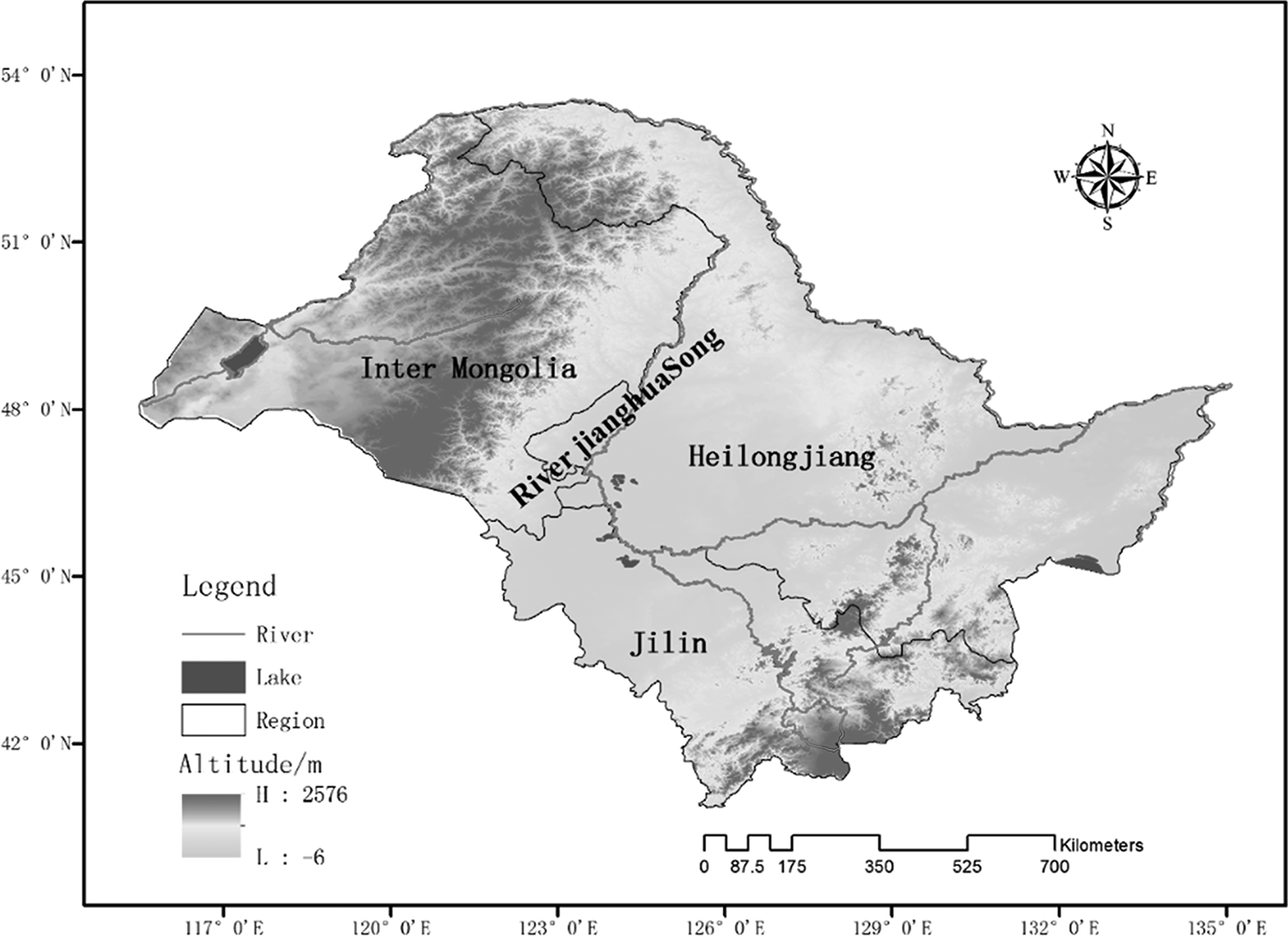
The Songhua River, one of the seven major rivers in China, is located at 41° 42′–51° 38′ N, 119° 52′–132° 31′ E, and it crosses the river basin's transboundary region, which spans the Inner Mongolia Autonomous Region and two provinces, namely Jilin and Heilongjiang (Fig. 2). The lengths of the main stream and the basin area are 939 km and 556,800 km2, respectively. The SRB is the most important source of water in the area, thereby influencing the sustainable economic and social development of the area (Yu et al., 2015b, 2016b). This area is occupied mostly by industrial production bases and relevant agricultural and grazing production bases. Pollution in the SRB is due to point source pollution from industrial and household wastewater discharges and from agricultural nonpoint source pollution induced by surface runoffs. Studies on temporal–spatial changes in the relationship of wastewater production, discharge, and wastewater treatment costs should be performed to improve the comprehensive control of water pollution in the SRB and to understand the intrinsic management of the basin.
Study area.
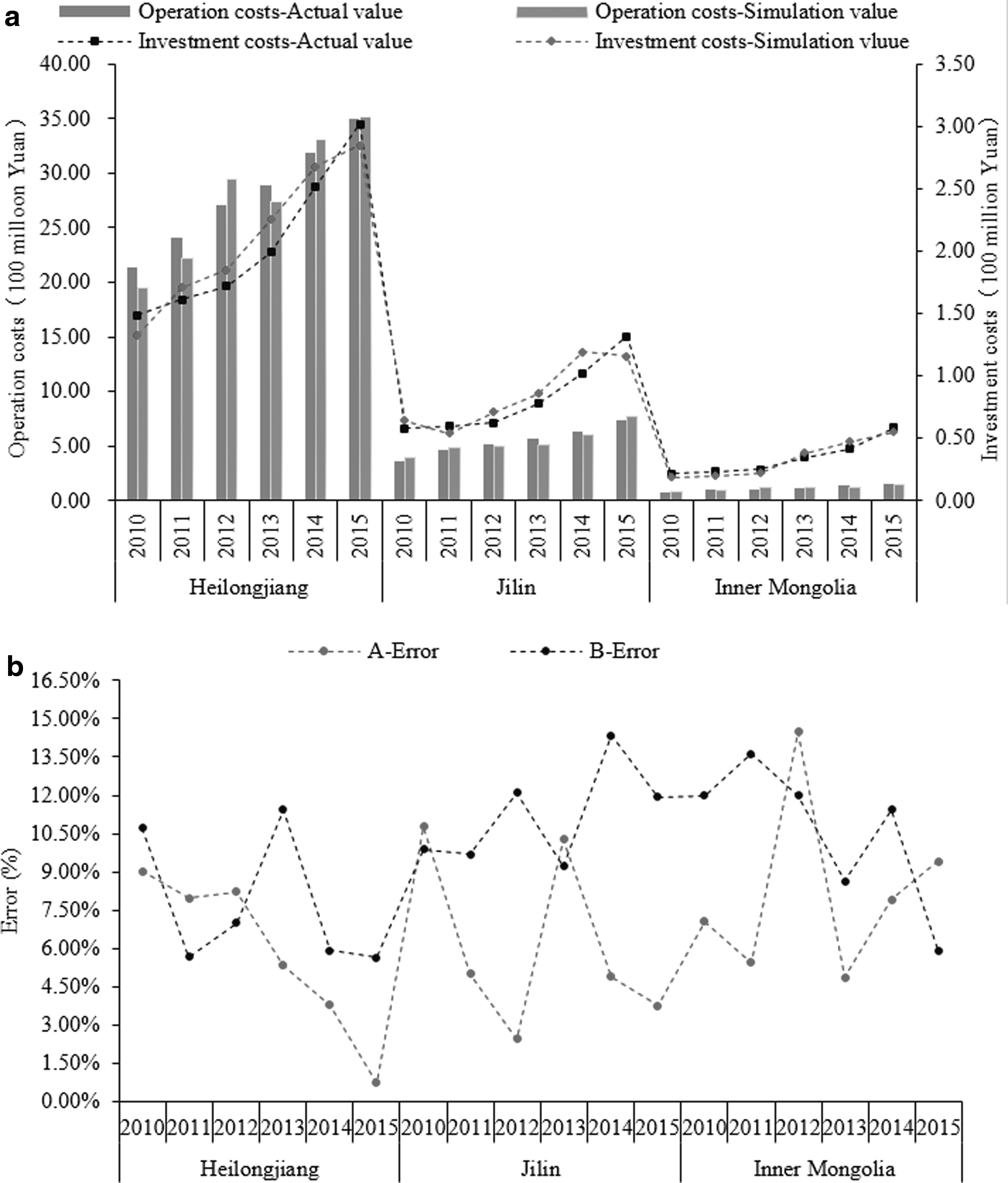
On the basis of the integrated predictive model of the transboundary river basin wastewater treatment costs established in this study, we simulated and predicted the wastewater discharge treatment investment costs (2010–2015) in the SRB and the transboundary region. The integrated predictive model of TRBTC was calculated using the linear planning computing program Lingo 11.0. Additional information on model training and verification, determined parameters, and intermediate results is not provided in this article because of editorial constraints. We also simulated and calculated the wastewater treatment costs (investment and operational) of the discharges from industrial areas, households, and raising livestock and poultry for the period 2010–2015 (abbr. simulated value). We then compared the simulated values with the historical data (Environmental Statistical Yearbook 2010–2015 of Heilongjiang, Jilin, and Inner Mongolia) (abbr. historical values) to validate the reasonability of the established model and the accuracy of the simulated results. Figures 3a, 4a, and 5a illustrate the compared results between the simulated values and the historical data from industrial areas, households, and raising livestock and poultry. Figures 3b, 4b, and 5b show the results of the relative error analysis between the simulated and historical values (|simulated value − historical value|/historical value). The relative errors between the two sets of values were less than 15%, indicating that the simulated results of the established model fitted well with the historical values. Therefore, the model could be used to simulate and predict the wastewater treatment costs in the SRB and its transboundary regions.
(a) Comparison of actual values and simulation values. (b) Error comparison of actual values and simulation values.
(a) Comparison of actual values and simulation values for industry. (b) Error comparison of actual values and simulation values for industry.
(a) Comparison of actual values and simulation values for urban household. (b) Error comparison of actual values and simulation values for urban household.
Simulation and prediction of industrial wastewater treatment costs
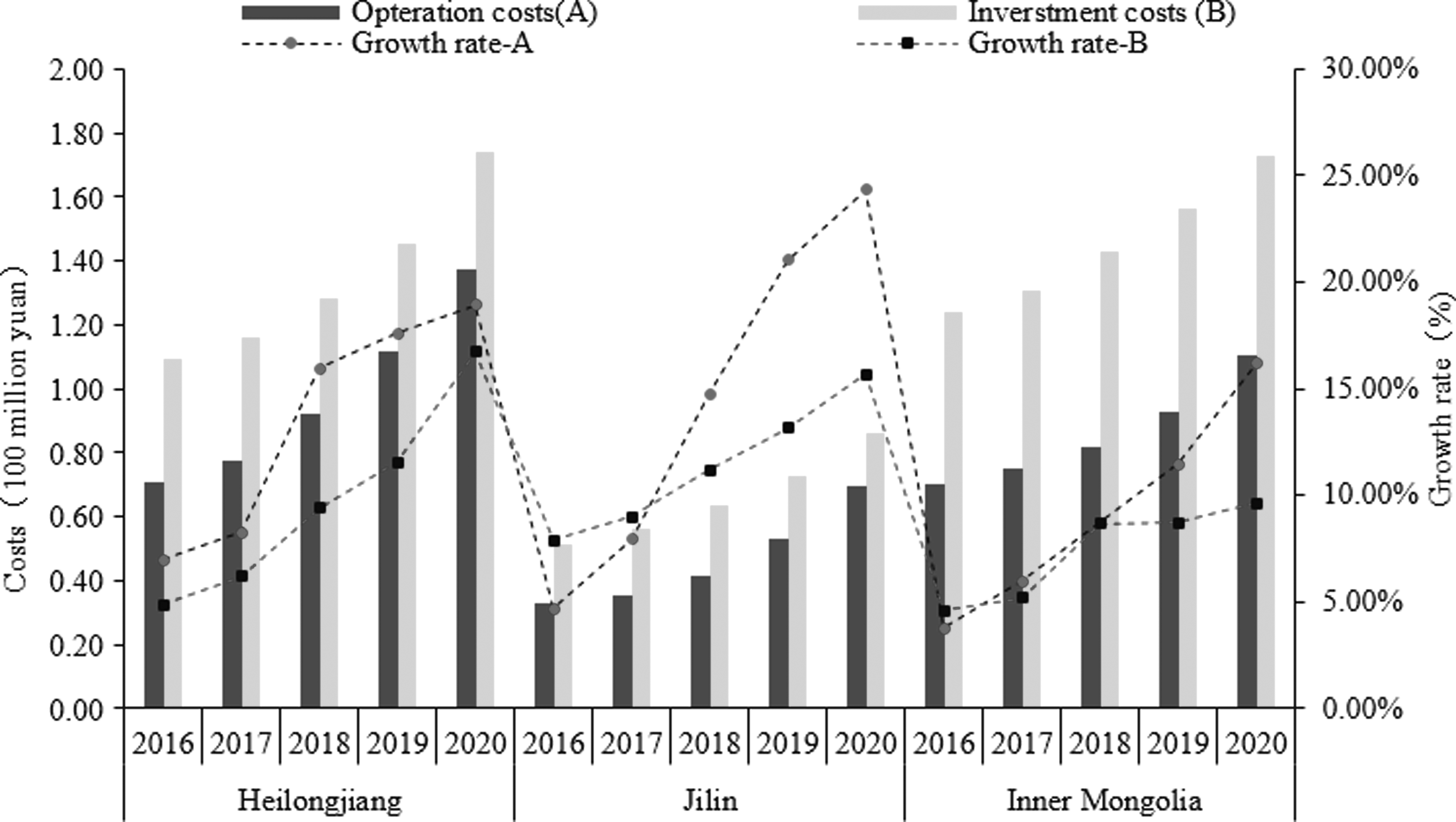
For the 13th Five-Year Plan's crucial stage of promoting the overall revitalization of old industrial bases in northeastern China, the energy structure was adjusted and the industry scale was optimized and accelerated. The energy consumption per 10,000 CNY GDP is far higher than the national ideal level, which is only 40–60% of the actual value in the area. Figure 6 shows the simulation and prediction results of the industrial wastewater treatment costs of the SRB for the period 2016–2020 by using the predictive model of industrial wastewater pollution treatment cost. The investment and operational costs of wastewater discharge pollution treatment presented an overall increasing trend during the 13th Five-Year Plan (China's 13th Five-year Plan of Water Pollution Prevention and Control in Key River Basins). In 2016, the industrial wastewater treatment operational costs of Heilongjiang, Jilin, and Inner Mongolia were 3.856 billion CNY, 0.847 billion CNY, and 0.194 billion CNY, respectively. The industrial wastewater investment costs of Heilongjiang, Jilin, and Inner Mongolia were 0.353 billion CNY, 0.153 billion CNY, and 0.073 billion CNY, respectively. In 2020, the industrial wastewater treatment operational costs of Heilongjiang, Jilin, and Inner Mongolia will be 6.935 billion CNY, 1.536 billion CNY, and 0.450 billion CNY, respectively. The industrial wastewater investment costs of Heilongjiang, Jilin, and Inner Mongolia will be 0.739 billion CNY, 0.307 billion CNY, and 0.182 billion CNY, respectively.
Simulation results of investment costs and operation costs for industry.
Compared with the costs during the 12th Five-Year Plan, the wastewater treatment operational costs of Heilongjiang, Jilin, and Inner Mongolia during the 13th Five-Year Plan increased by 44.40%, 44.86%, and 56.88%, respectively, and the investment costs increased by 52.51%, 50.04%, and 59.87%, respectively. The key industries in the SRB are electrical power, thermal production and supply, ferrous metal smelting and rolling, petroleum processing, coking and nuclear fuel processing, raw chemical material and chemical product manufacturing, papermaking and paper production, and agricultural and sideline product processing. Figure 7a indicates that the wastewater treatment operational costs of these six key industries in 2018 will account for 45.10%, 15.15%, 11.28%, 10.00%, 6.35%, and 4.12%, respectively, of the total operational costs. Figure 7b illustrates that the percentages of investment costs will account for 33.83%, 11.36%, 8.46%, 7.50%, 4.76%, and 3.09% of the total investment costs, respectively. Figure 8a shows that the percentages of the operational costs will be 46.25%, 16.03%, 11.04%, 11.03%, 6.10%, and 4.55% in 2020, respectively. Figure 8b displays that the percentages of the investment costs are 37.56%, 13.63%, 9.38%, 9.38%, 5.19%, and 3.87%, respectively.
(a) Comparison of operation costs of the key industries of Songhua River basin in 2018. (b) Comparison of investment costs of the key industries of Songhua River basin in 2018.
(a) Comparison of operation costs of the key industries of Songhua River basin in 2020. (b) Comparison of investment costs of the key industries of Songhua River basin in 2020.
Urban household wastewater treatment costs
Results of the evaluation of the basin water quality sections (China Environmental Status Bulletin 2010–2015) indicate that the most severe pollution was detected in the middle and downstream portions of the main stream of Songhua River and in the Second Songhua River. The large cities along the river have discharged large amounts of household and industrial wastewater, while creating an industrial output value, which caused the pollution of the surrounding river channels to be more severe compared with other channels. Figure 9 shows that the prediction results of investment costs and operation costs for urban household. In 2016, the urban household wastewater treatment operational costs and treatment investment costs of Heilongjiang were 0.555 billion CNY and 0.404 billion CNY, respectively. In 2016, the urban household wastewater treatment operational costs and treatment investment costs of Jilin were 0.458 billion CNY and 0.354 billion CNY, respectively. In 2016, urban household wastewater treatment operational costs and treatment investment costs of Inner Mongolia were 0.386 billion CNY and 0.287 billion CNY, respectively. In 2020, the urban household wastewater treatment operational costs and treatment investment costs of Heilongjiang will be 0.740 billion CNY and 0.514 billion CNY, respectively. In 2020, the urban household wastewater treatment operational costs and treatment investment costs of Jilin will be 0.563 billion CNY and 0.512 billion CNY, respectively. In 2020, the urban household wastewater treatment operational costs and treatment investment costs of Inner Mongolia will be 0.524 billion CNY and 0.389 billion CNY, respectively. Compared with the costs of the 12th Five-Year Plan, the urban household wastewater operational costs of Heilongjiang, Jilin, and Inner Mongolia increased by 24.97%, 18.71%, and 26.36%, respectively, while their treatment investment costs increased by 21.28%, 30.92%, and 26.30%, respectively.
Simulation results of investment costs and operation costs for urban household.
Wastewater treatment costs of raising livestock and poultry
With the acceleration of modern animal husbandry, the degree of large-scale husbandry in the SRB is continuously improving. However, the standardization degree has remained insufficient because excrement decontamination and utilization have lagged and caused severe environmental pollution. Figure 10 shows the prediction results of investment costs and operation costs for raising livestock and poultry. In 2016, the raising livestock and poultry wastewater treatment operational costs and treatment investment costs of Heilongjiang were 0.071 billion CNY and 0.109 billion CNY, respectively. In 2016, the raising livestock and poultry wastewater treatment operational costs and treatment investment costs of Jilin were 0.033 billion CNY and 0.051 billion CNY, respectively. In 2016, the raising livestock and poultry wastewater treatment operational costs and treatment investment costs of Inner Mongolia were 0.070 billion CNY and 0.124 billion CNY, respectively. In 2020, the raising livestock and poultry wastewater treatment operational costs and treatment investment costs of Heilongjiang will be 0.138 billion CNY and 0.174 billion CNY, respectively. In 2020, the raising livestock and poultry wastewater treatment operational costs and treatment investment costs of Jilin will be 0.070 billion CNY and 0.086 billion CNY, respectively. In 2020, the raising livestock and poultry wastewater treatment operational costs and treatment investment costs of Inner Mongolia will be 0.110 billion CNY and 0.173 billion CNY, respectively (Fig. 10). Compared with the costs during the 12th Five-Year Plan, the raising livestock and poultry wastewater operational costs of Heilongjiang, Jilin, and Inner Mongolia increased by 18.91%, 24.34%, and 16.17%, respectively, and their treatment investment costs increased by 16.74%, 15.69%, and 9.61%, respectively.
Simulation results of investment costs and operation costs for raising livestock and poultry.
The comprehensive analysis illustrated in Figs. 6, 9, and 10 reveals that during the 13th Five-Year Plan, wastewater treatment operational costs and investment costs of industrial, household, and raising livestock and poultry present an overall increasing trend. Among the total costs, the percentages of wastewater treatment operational and investment costs of were the greatest in Heilongjiang, followed by Jilin and Inner Mongolia. Compared with the costs during the 12th Five-Year Plan, the wastewater treatment investment costs and operational costs during the 13th Five-year Plan increased by 37.97% and 41.53%, respectively. With the continuous increase in wastewater treatment investment costs, the total wastewater discharge in the SRB would be effectively controlled and the quality of the aquatic environment would be effectively improved.
Conclusion
This study systematically established the coupling relationship of water resource utilization, water pollution discharge, and treatment costs in transboundary river basins. It also presented a comprehensive predictive model of TRBTC to conduct a temporal–spatial dynamic simulation of the changes in patterns of wastewater production, discharge, and treatment costs. The model's main advantage is its ability to quantify the characteristic change in economic growth and wastewater discharge pollution treatment costs. This study also provided a scientific basis for decision making for wastewater discharge control and management in transboundary river basins. This study could also offer references for water pollution control and for the simulation and prediction of water pollution treatment investment costs in other transboundary river basins.
The SRB was selected as the study area, and the comprehensive predictive model of TRBTC proposed in this article was utilized to conduct a temporal–spatial dynamic simulation of the changes in patterns of wastewater production, discharge, and treatment costs. According to the simulation results, the overall pattern of wastewater treatment operational and investment costs in the SRB was increasing, that is, the costs during the 13th Five-Year Plan, respectively, increased by 41.53% and 37.97% compared with those during the 12th Five-Year Plan. With the continuous increase in treatment investment costs, the total water pollutant discharge in the SRB has been effectively controlled and water quality has evidently improved.
This study explored the dynamic changes in patterns of related economic growth and wastewater discharge pollution treatment costs, described practical applications, and conducted a model simulation and prediction of the SRB and its transboundary region. Our results validated the feasibility, reasonability, and operability of the established model. The established comprehensive and predictive model of transboundary river basin wastewater treatment costs were based on a series of theoretical derivations and simplification of actual and complex problems because the influence of transboundary river basin wastewater pollution on the basin's social and economic development was complex. We expected that the established model could be continuously improved with repeated practical applications and increasing enrichment of fundamental material accumulation. Compared with most of the other commonly used models and implementation frameworks, the novel feature of the proposed approach and framework is the strong ability to address many challenges essential for further research and practical applications.
Footnotes
Acknowledgments
This research was supported by China Postdoctoral Science Foundation (NO.2016M591139), the Fundamental Research Funds for the Central Universities–China (NO.JB2016072), the Major Science and Technology Program for Water Pollution Control and Treatment (NO.2012ZX07601002), and the Program for China National Funds for Excellent Young Scientists (NO.51422903).
Author Disclosure Statement
No competing financial interests exist.
References
1.
AhnJ., and KangD. (2014). Optimal planning of water supply system for long-term sustainability. J. Hydro Environ. Res., 8, 410.
2.
AtabM.S., SmallboneA.J., and RoskillyA.P. (2016). An operational and economic study of a reverse osmosis desalination system for potable water and land irrigation. Desalination, 397, 174.
3.
ChettyS., and PillayK. (2015). Application of the DIY carbon footprint calculator to a wastewater treatment works. Water SA. 41, 263.
4.
DegefuD.M., HeW.J., YuanL., et al. (2016). Water allocation in transboundary river basins under water scarcity: A cooperative bargaining approach. Water Resour. Manag., 30, 4451.
5.
DjukicM., JovanoskiI., IvanovicO.M., et al. (2016). Cost-benefit analysis of an infrastructure project and a cost-reflective tariff: A case study for investment in wastewater treatment plant in Serbia. Renew. Sustain. Energy Rev., 59, 1419.
6.
DoreJ., LebelL., and MolleF. (2012). A framework for analysing transboundary water governance complexes, illustrated in the Mekong Region. J. Hydrol., 466, 23.
7.
EggimannS., TrufferB., and MaurerM. (2016). Economies of density for on-site waste water treatment. Water Res. 101, 476.
8.
El-GoharyF.A., NasrF.A., WahaabR.A., et al. (2013). Cost-effective pre-treatment of agro-industrial wastewater. Water Sci. Technol., 11, 297.
9.
GeH., BatstoneD.J., and KellerJ. (2013). Operating aerobic wastewater treatment at very short sludge ages enables treatment and energy recovery through anaerobic sludge digestion. Water Res. 47, 6546.
10.
HautakangasS., OllikainenM., AarnosK., et al. (2014). Nutrient abatement potential and abatement costs of waste water treatment plants in the Baltic Sea Region. Ambio, 43, 352.
11.
HeatherN.B., JustinE.L., BrianJ.H., et al. (2013). Renewing urban streams with recycled water for streamflow augmentation: Hydrologic, water ouality, and ecosystem services management. Environ. Eng. Sci., 30, 455.
12.
Hernandez-SanchoF., Molinos-SenanteM., and Sala-GarridoR. (2011). Cost modelling for wastewater treatment processes. Desalination, 268, 1.
13.
JorsaraeiA., GougolM., and LierJ.B.V. (2013). A cost effective method for decentralized sewage treatment. Process Saf. Environ. Prot., 92, 815.
14.
KearnsJ.P., KnappeD.R.U., and SummersR.S. (2015). Feasibility of using traditional kiln charcoals in low-cost water treatment: Role of pyrolysis conditions on 2, 4-D herbicide adsorption. Environ. Eng. Sci., 32, 912.
15.
KucukmehmetogluM. (2012). An integrative case study approach between game theory and Pareto frontier concepts for the transboundary water resources allocations. J. Hydrol., 450, 308.
16.
KurtM., AksoyA., and SaninF.D. (2015). Evaluation of solar sludge drying alternatives by costs and area requirements. Water Res. 82, 47.
17.
LangeC., SchneiderM., MutzM., et al. (2015). Model-based design for restoration of a small urban river. J. Hydro Environ. Res., 9, 226.
18.
LiJ., DongQ., LiuL., et al. (2016). Measuring treatment costs of typical waste electrical and electronic equipment: A pre-research for Chinese policy making. Waste Manag. 57, 36.
19.
LiuJ.K., WangY.S., ZhangW.J., et al. (2014). Cost-benefit analysis of construction and demolition waste management based on system dynamics: A case study of Guangzhou. Syst. Eng. Theory Practice, 34, 1480.
20.
LogarI., BrouwerR., MaurerM., et al. (2014). Cost-benefit analysis of the swiss national policy on reducing micropollutants in treated wastewater. Environ. Sci. Technol., 48, 12500.
21.
MalakoffD. (2011). Can treatment costs be tamed?. Science. 331, 1545.
22.
MalmA., MobergF., RosénL., et al. (2015). Cost-benefit analysis and uncertainty analysis of water loss reduction measures: Case study of the Gothenburg drinking water distribution System. Water Res. Manag., 29, 5451.
23.
MarzoukM., and ElkadiM. (2016). Estimating water treatment plants costs using factor analysis and artificial neural networks. J. Clean. Prod., 112, 4540.
24.
MohammadA.A., MalihehF., and SadeghB. (2011). Multivariate econometric approach for solid waste generation modeling: Impact of climate factors. Environ. Eng. Sci., 28, 627.
25.
Molinos-SenanteM., Hernández-SanchoF., and Sala-GarridoR. (2011). Cost-benefit analysis of water-reuse projects for environmental purposes: A case study for Spanish wastewater treatment plants. J. Environ. Manag., 92, 3091.
26.
MorenoR., SanmartínM.I., EscapaA., et al. (2016). Domestic wastewater treatment in parallel with methane production in a microbial electrolysis cell. Renew. Energy, 93, 442.
27.
NiuK., WuJ., YuF., et al. (2016). Construction and operation costs of wastewater treatment and implications for the paper industry in China. Environ. Sci. Technol., 50, 12339.
28.
PérezJ.A.S., SánchezI.M.R., CarraI., et al. (2012). Economic evaluation of a combined photo-Fenton/MBR process using pesticides as model pollutant. Factors affecting costs. J. Hazard. Mater. 244–245:195–203.
29.
RinaudoJ.D., and AulongS. (2014). Defining groundwater remediation objectives with cost-benefit analysis: Does it work? Water Res. Manag. 28:261.
30.
RocherV., PaffoniC., GonçalvesA., et al. (2012). Municipal wastewater treatment by biofiltration: Comparisons of various treatment layouts. Part 2: Assessment of the operating costs in optimal conditions. Water Sci. Technol., 65, 1713.
31.
RodriguezgarciaG., MolinossenanteM., HospidoA., et al. (2011). Environmental and economic profile of six typologies of wastewater treatment plants. Water Res. 45, 5997.
32.
Ruiz-RosaI., García-RodríguezF.J., and Mendoza-JiménezJ. (2016). Development and application of a cost management model for wastewater treatment and reuse processes. J. Clean. Prod., 113, 299.
33.
ShihY.H., and TsengC.H. (2014). Cost-benefit analysis of sustainable energy development using life-cycle co-benefits assessment and the system dynamics approach. Appl. Energy, 119, 57.
34.
WangY., WangP., BaiY.J., et al. (2013). Assessment of surface water quality via multivariate statistical techniques: A case study of the Songhua River Harbin region, China. J. Hydro Environ. Res., 7, 30.
35.
YuS., HeL., and LuH. (2016a). A tempo-spatial-distributed multi-objective decision-making model for ecological restoration management of water-deficient rivers. J. Hydrol., 542, 860.
36.
YuS., HeL., and LuH.W. (2016b). An environmental fairness based optimisation model for the decision-support of joint control over the water quantity and quality of a river basin. J. Hydrol., 535, 366.
37.
YuS., JiangH.Q., and ChangM. (2015a). Integrated prediction model for optimizing distributions of total amount of water pollutant discharge in the Songhua River watershed. Stoch. Environ. Res. Risk Assess., 30, 2179.
38.
YuS., JiangH.Q., ChangM., et al. (2015b). Dynamic simulation scheme on integrated control of water resources and water pollution in the Songhua river basin. Acta Sci. Circumst., 35, 1866.
39.
ZhaoW.Y., ZhangF., Hong-YingH.U., et al. (2012). Analysis on construction cost of ozone oxidation process for wastewater advanced treatment and reuse. Environ. Sci. Technol., 35, 139.
40.
ZhouC., GongZ., HuJ., et al. (2015). A cost-benefit analysis of landfill mining and material recycling in China. Waste Manag. 35, 191.
Supplementary Material
Please find the following supplemental material available below.
For Open Access articles published under a Creative Commons License, all supplemental material carries the same license as the article it is associated with.
For non-Open Access articles published, all supplemental material carries a non-exclusive license, and permission requests for re-use of supplemental material or any part of supplemental material shall be sent directly to the copyright owner as specified in the copyright notice associated with the article.