In this study, an interval double-sided fuzzy chance-constrained programming (IDFCP) approach is developed for identifying water resources allocation strategies under uncertainty. Through incorporating interval parameter programming, double-sided fuzzy programming, and chance-constrained programming into a general framework, IDFCP can effectively deal with uncertainties expressed as intervals, probability distributions, and fuzzy sets. IDFCP can also examine the risk of violating system constraints. IDFCP is then applied to water resources allocation in the middle and upper reaches of Fen River Basin that is associated with multiuser, multiregion, and multisource features. Interval solutions of the compromise decision alternatives are generated under different scenarios in association with different risk levels of violating constraints (i.e., p levels), fuzzy membership degrees (i.e., α-cut levels), credible degrees (i.e., minimum and maximum), and reclaimed water utilization ratios. Results obtained show that water availability can affect water allocation pattern and system benefit. Results are helpful for decision makers to identify desirable strategies under various environmental and system-credibility constraints in more profitable and sustainable ways.
Introduction
Water resources management is one of the most critical global issues, since water resources have strong relationships with all aspects of people's livelihood and environmental sustainability (Li et al., 2010; Daysan et al., 2017). However, uneven temporal and spatial distributions of water resources, climate change, as well as human activities have caused severe water shortage problems that has threatened human health, blocked the socioeconomic development, and destroyed the maintenance of ecosystems (Cai et al., 2011; Dou and Wang, 2017). In addition, the growing population, rapid industrialization, and the extensive agricultural reclamation have resulted in increasing demands on water resources (Fan et al., 2015; Oxley and Mays, 2016). Thus, the management of water resources has become an increasingly pressing issue in many regions (Huang et al., 2010).
Water resources management is complicated, involving a number of factors such as economy, environment, and politics. The optimization technique has proven efficient for balancing the trade-offs among these influencing factors and managing limited water resources in a sustainable way (Xu et al., 2009; Housh et al., 2013). However, water resources management system is plagued with multiple uncertainties and complexities due to the random features of stream conditions, the errors in estimated modeling parameters (e.g., water demand), the vagueness of system (e.g., loss coefficient), and the interaction among the water resources system components (Li and Huang, 2008; Hassanzadeh et al., 2016). These uncertainties and complexities would bring a series of decision-making risks and difficulties (Wang et al., 2017). To identify robust strategies for water resources utilization confronted with these uncertainties, it is desired to formulate effective tools for supporting sustainable water resources management.
Background
Previously, a number of optimization methods were developed to deal with uncertainties existing in water resources allocation problems. The majority of them are related to chance-constrained programming (CCP) and fuzzy mathematical programming (FMP) (Chaves et al., 2003; Li et al., 2009). FMP could deal with vagueness and ambiguity in the objective and constraints (Maqsood et al., 2005; Li et al., 2010); CCP is capable of handling probabilistic distributions on the right-hand side of constraints (Martinez and Anderson, 2015).
Chance-constrained programming
CCP is useful for providing information on the trade-offs between the objective function value and the probability of satisfying the constraints (Cao et al., 2009; Aiche et al., 2013). Kwon et al. (2009) developed a CCP approach for planning the irrigation water resources in Korea. Tan et al. (2011) used a CCP model to develop an agricultural water resources management plan in a polluted area corresponding to varied risk levels of constraint. Sreekanth et al. (2012) developed a CCP model to derive long-term water resources operation strategies for a reservoir in South India. Ji et al. (2014) used CCP for dealing with random variables in an agricultural water resources system. Nima and Frank (2015) formulated a CCP model for promoting the groundwater remediation designs to analyze the impact of uncertainties on the remediation design; the obtained results indicate that CCP is capable of handling decision problems under right-hand stochastic constraints. However, in many situations, the probability distribution is determined via tests, experiences, and expertise, while these methods may fail in determining accurate values for the probability distribution, leading to probability distribution being described by fuzzy linear inequalities (Abdelaziz et al., 2004). Such deviations in subjective estimations can result in fuzziness and randomness being inherent in the real-world decision problems, neglect of which can cause the solutions of problems deviating greatly from their real conditions (Eslami et al., 2012; Li et al., 2014).
Fuzzy mathematical programming
FMP considers uncertainties expressed as fuzzy sets and is a flexible approach that can effectively reflect ambiguity and vagueness in water resources management systems (Kamodkar and Regular, 2013; Lence et al., 2017). Uddameri et al. (2014) used the FMP for estimating optimal groundwater availability with an objective of maximizing groundwater production. Zhou et al. (2016) used an FMP method for supporting water resources management system, in which different α-cut levels are assigned to each fuzzy parameter. Dutta et al. (2016) proposed an FMP model for planning irrigation water resources management system and determining the optimum cropping patterns for the next crop season. FMP is an alternative for solving the uncertainties expressed as fuzzy sets; however, it may encounter difficulty in dealing with probabilistic distributions in a nonfuzzy decision space (Liu et al., 2009).
Fuzzy chance-constrained programming
Fuzzy chance-constrained programming (FCP) is effective for dealing with fuzzy sets and probability distributions through integrating FMP and CCP into a general framework. Abdelaziza et al. (2004) developed an FCP approach for solving fuzzy and stochastic parameters in water resources management to determine reservoir releases in the Ichkeul Basin. Pal et al. (2011) proposed an FCP method for dealing with uncertainties expressed as fuzzy sets, such as utilization of total cultivable land in an agricultural water resource system. Guo et al. (2014) developed an FCP linear programming approach for managing agricultural water resources. Xu et al. (2017) proposed an FCP model to tackle the uncertainties expressed as fuzzy sets and probability distributions and to reflect the tradeoffs between economic revenues and system failure risk. In general, based on given probabilities of constraint violations, FCP could not only be used to reflect the trade-off between objective function and the system risk level but also to effectively address fuzzy sets on single side of the constraints. However, the conventional FCP has difficulties in tackling uncertainties on both sides of the model's constraints such as the loss coefficient and the amount of available water, which would be expressed as fuzzy sets on both sides of constraints, respectively (Cui et al., 2016).
Objective
Therefore, this study aims to develop an interval double-sided fuzzy chance-constrained programming (IDFCP) method for planning water resources system through integrating CCP, FMP, and interval parameter programming (IPP) approach into the general framework. IDFCP can handle uncertainties expressed as probability distributions, interval values, and fuzzy sets on both sides of the constraints; it also allows examining risks of system constraint violation at specified confidence levels. Minimum credibility and maximum credibility are used to deal with fuzzy information. Then, IDFCP will be applied to planning water resources allocation in the middle and upper reaches of Fen River. The results will be useful for generating a range of decision alternatives under various uncertainties and help decision makers identify desired water resources allocation alternatives.
Methodology
Chance-constrained programming
CCP is useful for dealing with random uncertainty and reflecting the information risk of violating constraints (Charnes and Cooper, 1983). A general CCP problem is presented as follows:
\documentclass{aastex}\usepackage{amsbsy}\usepackage{amsfonts}\usepackage{amssymb}\usepackage{bm}\usepackage{mathrsfs}\usepackage{pifont}\usepackage{stmaryrd}\usepackage{textcomp}\usepackage{portland, xspace}\usepackage{amsmath, amsxtra}\usepackage{upgreek}\pagestyle{empty}\DeclareMathSizes{10}{9}{7}{6}\begin{document}
\begin{align*}
Max \ f = CX , \tag{1a}
\end{align*}
\end{document}
subject to:
\documentclass{aastex}\usepackage{amsbsy}\usepackage{amsfonts}\usepackage{amssymb}\usepackage{bm}\usepackage{mathrsfs}\usepackage{pifont}\usepackage{stmaryrd}\usepackage{textcomp}\usepackage{portland, xspace}\usepackage{amsmath, amsxtra}\usepackage{upgreek}\pagestyle{empty}\DeclareMathSizes{10}{9}{7}{6}\begin{document}
\begin{align*}
pr [ \{ t \left\vert {{A_i} ( t ) X \le {B_i} ( t ) } \right. \} ] \ge 1 - {p_i} ,\, {A_i} ( t ) \in A ( t ) ,\, i = 1 , 2 , \ldots , m , \tag{1b}
\end{align*}
\end{document}\documentclass{aastex}\usepackage{amsbsy}\usepackage{amsfonts}\usepackage{amssymb}\usepackage{bm}\usepackage{mathrsfs}\usepackage{pifont}\usepackage{stmaryrd}\usepackage{textcomp}\usepackage{portland, xspace}\usepackage{amsmath, amsxtra}\usepackage{upgreek}\pagestyle{empty}\DeclareMathSizes{10}{9}{7}{6}\begin{document}
\begin{align*}
DX \ge E , \tag{1c}
\end{align*}
\end{document}\documentclass{aastex}\usepackage{amsbsy}\usepackage{amsfonts}\usepackage{amssymb}\usepackage{bm}\usepackage{mathrsfs}\usepackage{pifont}\usepackage{stmaryrd}\usepackage{textcomp}\usepackage{portland, xspace}\usepackage{amsmath, amsxtra}\usepackage{upgreek}\pagestyle{empty}\DeclareMathSizes{10}{9}{7}{6}\begin{document}
\begin{align*}
{X_j} \ge 0 , {x_j} \in X , \,j = 1 , 2 , \ldots , n , \tag{1d}
\end{align*}
\end{document}
where x is a vector of decision variables; f is objective function; A(t), B(t), and C are sets with random elements defined on a probability space T, t\documentclass{aastex}\usepackage{amsbsy}\usepackage{amsfonts}\usepackage{amssymb}\usepackage{bm}\usepackage{mathrsfs}\usepackage{pifont}\usepackage{stmaryrd}\usepackage{textcomp}\usepackage{portland, xspace}\usepackage{amsmath, amsxtra}\usepackage{upgreek}\pagestyle{empty}\DeclareMathSizes{10}{9}{7}{6}\begin{document}
$$\in$$
\end{document}T. Model (1) consists of fixing a certain level of probability pi\documentclass{aastex}\usepackage{amsbsy}\usepackage{amsfonts}\usepackage{amssymb}\usepackage{bm}\usepackage{mathrsfs}\usepackage{pifont}\usepackage{stmaryrd}\usepackage{textcomp}\usepackage{portland, xspace}\usepackage{amsmath, amsxtra}\usepackage{upgreek}\pagestyle{empty}\DeclareMathSizes{10}{9}{7}{6}\begin{document}
$$\in$$
\end{document} [0, 1] for each constraint i and imposing a condition that the constraint is satisfied with at least a probability of 1−pi (Infanger and Morton, 1996; Xie et al., 2011). An “equivalent” deterministic version can be defined when the left-hand side coefficients aij are deterministic and bi are random. Equation (1b) can be transformed to an equivalent linear (Xie et al., 2011):
\documentclass{aastex}\usepackage{amsbsy}\usepackage{amsfonts}\usepackage{amssymb}\usepackage{bm}\usepackage{mathrsfs}\usepackage{pifont}\usepackage{stmaryrd}\usepackage{textcomp}\usepackage{portland, xspace}\usepackage{amsmath, amsxtra}\usepackage{upgreek}\pagestyle{empty}\DeclareMathSizes{10}{9}{7}{6}\begin{document}
\begin{align*}
{A_i} ( t ) X \le {b_i}{ ( t ) ^{ ( {p_i} ) }} , \forall i , \tag{2a}
\end{align*}
\end{document}
where bi(t)(pi) = Fi−1(pi), in which Fi(pi) is the cumulative distribution function of bi and pi is the probability of violating constraint i.
Double-sided FCP
The FCP approach has been successfully used in many applications. However, in many real-world management problems, it is more common that both sides of constraints will be associated with fuzzy sets. Thus, it is desired more competent methods be advanced due to the limitation of FCP. Consequently, a double-sided fuzzy chance-constrained programming (DFCP) approach is developed to address the deficiency. The DFCP approach can be formulated as follows (Inuiguchi and Ramik, 2000):
subject to:
\documentclass{aastex}\usepackage{amsbsy}\usepackage{amsfonts}\usepackage{amssymb}\usepackage{bm}\usepackage{mathrsfs}\usepackage{pifont}\usepackage{stmaryrd}\usepackage{textcomp}\usepackage{portland, xspace}\usepackage{amsmath, amsxtra}\usepackage{upgreek}\pagestyle{empty}\DeclareMathSizes{10}{9}{7}{6}\begin{document}
\begin{align*}
pr \{ \omega \vert { \tilde A} ( \omega ) X \le \tilde B ( \omega ) X \} \ge 1 - p , \tag{3b}
\end{align*}
\end{document}\documentclass{aastex}\usepackage{amsbsy}\usepackage{amsfonts}\usepackage{amssymb}\usepackage{bm}\usepackage{mathrsfs}\usepackage{pifont}\usepackage{stmaryrd}\usepackage{textcomp}\usepackage{portland, xspace}\usepackage{amsmath, amsxtra}\usepackage{upgreek}\pagestyle{empty}\DeclareMathSizes{10}{9}{7}{6}\begin{document}
\begin{align*}
DX \ge E , \tag{3c}
\end{align*}
\end{document}\documentclass{aastex}\usepackage{amsbsy}\usepackage{amsfonts}\usepackage{amssymb}\usepackage{bm}\usepackage{mathrsfs}\usepackage{pifont}\usepackage{stmaryrd}\usepackage{textcomp}\usepackage{portland, xspace}\usepackage{amsmath, amsxtra}\usepackage{upgreek}\pagestyle{empty}\DeclareMathSizes{10}{9}{7}{6}\begin{document}
\begin{align*}
X \ge 0 , \tag{3d}
\end{align*}
\end{document}\documentclass{aastex}\usepackage{amsbsy}\usepackage{amsfonts}\usepackage{amssymb}\usepackage{bm}\usepackage{mathrsfs}\usepackage{pifont}\usepackage{stmaryrd}\usepackage{textcomp}\usepackage{portland, xspace}\usepackage{amsmath, amsxtra}\usepackage{upgreek}\pagestyle{empty}\DeclareMathSizes{10}{9}{7}{6}\begin{document}
\begin{align*}
C , { \tilde A} \ne 0. \tag{3e}
\end{align*}
\end{document}
\documentclass{aastex}\usepackage{amsbsy}\usepackage{amsfonts}\usepackage{amssymb}\usepackage{bm}\usepackage{mathrsfs}\usepackage{pifont}\usepackage{stmaryrd}\usepackage{textcomp}\usepackage{portland, xspace}\usepackage{amsmath, amsxtra}\usepackage{upgreek}\pagestyle{empty}\DeclareMathSizes{10}{9}{7}{6}\begin{document}
$${ \tilde A}$$
\end{document} and \documentclass{aastex}\usepackage{amsbsy}\usepackage{amsfonts}\usepackage{amssymb}\usepackage{bm}\usepackage{mathrsfs}\usepackage{pifont}\usepackage{stmaryrd}\usepackage{textcomp}\usepackage{portland, xspace}\usepackage{amsmath, amsxtra}\usepackage{upgreek}\pagestyle{empty}\DeclareMathSizes{10}{9}{7}{6}\begin{document}
$${ \tilde B}$$
\end{document} are vectors expressed as fuzzy set with membership functions \documentclass{aastex}\usepackage{amsbsy}\usepackage{amsfonts}\usepackage{amssymb}\usepackage{bm}\usepackage{mathrsfs}\usepackage{pifont}\usepackage{stmaryrd}\usepackage{textcomp}\usepackage{portland, xspace}\usepackage{amsmath, amsxtra}\usepackage{upgreek}\pagestyle{empty}\DeclareMathSizes{10}{9}{7}{6}\begin{document}
$$\mu ( { \tilde A} )$$
\end{document} and equation \documentclass{aastex}\usepackage{amsbsy}\usepackage{amsfonts}\usepackage{amssymb}\usepackage{bm}\usepackage{mathrsfs}\usepackage{pifont}\usepackage{stmaryrd}\usepackage{textcomp}\usepackage{portland, xspace}\usepackage{amsmath, amsxtra}\usepackage{upgreek}\pagestyle{empty}\DeclareMathSizes{10}{9}{7}{6}\begin{document}
$$\mu ( \tilde B )$$
\end{document}, respectively. Equation (3b) is a fuzzy chance constraint that can be violated at specified confidence levels.
In model (3), each predetermined confidence level consists of two scenarios that are minimum credibility and maximum credibility (Fiedler et al., 2006; Xu and Qin, 2010). The constraints would be more relaxed through using the minimum credibility to deal with fuzzy sets. However, they would be narrower by using maximum credibility to address fuzzy sets. Thus, it is capable of addressing different decision makers' personal judgments or experiences and provides more decision-making options for decision makers. Generally, Equation (3b) can be formulated as follows:
\documentclass{aastex}\usepackage{amsbsy}\usepackage{amsfonts}\usepackage{amssymb}\usepackage{bm}\usepackage{mathrsfs}\usepackage{pifont}\usepackage{stmaryrd}\usepackage{textcomp}\usepackage{portland, xspace}\usepackage{amsmath, amsxtra}\usepackage{upgreek}\pagestyle{empty}\DeclareMathSizes{10}{9}{7}{6}\begin{document}
\begin{align*}
\begin{split}pr \{ \tilde a\ \tilde \le \ ^{ \min } \,\tilde b \} = \sup \ \{ \min ( { \mu _{ \tilde a}} ( x ) , { \mu _{ \tilde b}} ( y ) ) \vert x , y \in R , x \le y \} ,\end{split}
\tag{4a}
\end{align*}
\end{document}\documentclass{aastex}\usepackage{amsbsy}\usepackage{amsfonts}\usepackage{amssymb}\usepackage{bm}\usepackage{mathrsfs}\usepackage{pifont}\usepackage{stmaryrd}\usepackage{textcomp}\usepackage{portland, xspace}\usepackage{amsmath, amsxtra}\usepackage{upgreek}\pagestyle{empty}\DeclareMathSizes{10}{9}{7}{6}\begin{document}
\begin{align*}
\begin{split}pr \{ \tilde a\ \tilde\le\ {^{ \max }} \,\tilde b \} = \sup \ \{ \max ( 1 - { \mu _{ \tilde a}} ( x ) , \\ \quad1 - { \mu _{ \tilde b}} ( y ) ) \vert x , y \in R ,\, x \le y \} ,\end{split}
\tag{4b}
\end{align*}
\end{document}
where \documentclass{aastex}\usepackage{amsbsy}\usepackage{amsfonts}\usepackage{amssymb}\usepackage{bm}\usepackage{mathrsfs}\usepackage{pifont}\usepackage{stmaryrd}\usepackage{textcomp}\usepackage{portland, xspace}\usepackage{amsmath, amsxtra}\usepackage{upgreek}\pagestyle{empty}\DeclareMathSizes{10}{9}{7}{6}\begin{document}
$$\tilde a \, \tilde \le \ {^{ \min }} \; {\tilde b}$$
\end{document} presents that the equation \documentclass{aastex}\usepackage{amsbsy}\usepackage{amsfonts}\usepackage{amssymb}\usepackage{bm}\usepackage{mathrsfs}\usepackage{pifont}\usepackage{stmaryrd}\usepackage{textcomp}\usepackage{portland, xspace}\usepackage{amsmath, amsxtra}\usepackage{upgreek}\pagestyle{empty}\DeclareMathSizes{10}{9}{7}{6}\begin{document}
$$\tilde a \le \tilde b$$
\end{document} should be satisfied at the minimum credibility; \documentclass{aastex}\usepackage{amsbsy}\usepackage{amsfonts}\usepackage{amssymb}\usepackage{bm}\usepackage{mathrsfs}\usepackage{pifont}\usepackage{stmaryrd}\usepackage{textcomp}\usepackage{portland, xspace}\usepackage{amsmath, amsxtra}\usepackage{upgreek}\pagestyle{empty}\DeclareMathSizes{10}{9}{7}{6}\begin{document}
$$\tilde a\ \tilde \le \ {^{ \max }} \ {\tilde b}$$
\end{document} means that the equation \documentclass{aastex}\usepackage{amsbsy}\usepackage{amsfonts}\usepackage{amssymb}\usepackage{bm}\usepackage{mathrsfs}\usepackage{pifont}\usepackage{stmaryrd}\usepackage{textcomp}\usepackage{portland, xspace}\usepackage{amsmath, amsxtra}\usepackage{upgreek}\pagestyle{empty}\DeclareMathSizes{10}{9}{7}{6}\begin{document}
$${\tilde a} \le {\tilde b}$$
\end{document} should be satisfied at the maximum credibility. Equation (4a) means that the possibility of \documentclass{aastex}\usepackage{amsbsy}\usepackage{amsfonts}\usepackage{amssymb}\usepackage{bm}\usepackage{mathrsfs}\usepackage{pifont}\usepackage{stmaryrd}\usepackage{textcomp}\usepackage{portland, xspace}\usepackage{amsmath, amsxtra}\usepackage{upgreek}\pagestyle{empty}\DeclareMathSizes{10}{9}{7}{6}\begin{document}
$$\tilde a \le \tilde b$$
\end{document} is the possibility that there exists at least one pair of values x, y ∈ R such that \documentclass{aastex}\usepackage{amsbsy}\usepackage{amsfonts}\usepackage{amssymb}\usepackage{bm}\usepackage{mathrsfs}\usepackage{pifont}\usepackage{stmaryrd}\usepackage{textcomp}\usepackage{portland, xspace}\usepackage{amsmath, amsxtra}\usepackage{upgreek}\pagestyle{empty}\DeclareMathSizes{10}{9}{7}{6}\begin{document}
$$x \le y$$
\end{document}, and specified values of \documentclass{aastex}\usepackage{amsbsy}\usepackage{amsfonts}\usepackage{amssymb}\usepackage{bm}\usepackage{mathrsfs}\usepackage{pifont}\usepackage{stmaryrd}\usepackage{textcomp}\usepackage{portland, xspace}\usepackage{amsmath, amsxtra}\usepackage{upgreek}\pagestyle{empty}\DeclareMathSizes{10}{9}{7}{6}\begin{document}
$$\tilde a$$
\end{document} and \documentclass{aastex}\usepackage{amsbsy}\usepackage{amsfonts}\usepackage{amssymb}\usepackage{bm}\usepackage{mathrsfs}\usepackage{pifont}\usepackage{stmaryrd}\usepackage{textcomp}\usepackage{portland, xspace}\usepackage{amsmath, amsxtra}\usepackage{upgreek}\pagestyle{empty}\DeclareMathSizes{10}{9}{7}{6}\begin{document}
$$\tilde b$$
\end{document} are x and y, respectively (Liu and Iwamura, 1998). Conversely, the meaning of Equation (4b) is opposite to that of Equation (4a).
Based on Equations (4a) and (4b), for any given 1 − p ∈ (0, 1), the following two equations can be derived:
\documentclass{aastex}\usepackage{amsbsy}\usepackage{amsfonts}\usepackage{amssymb}\usepackage{bm}\usepackage{mathrsfs}\usepackage{pifont}\usepackage{stmaryrd}\usepackage{textcomp}\usepackage{portland, xspace}\usepackage{amsmath, amsxtra}\usepackage{upgreek}\pagestyle{empty}\DeclareMathSizes{10}{9}{7}{6}\begin{document}
\begin{align*}
\begin{split} pr \{ \tilde a\ \tilde \le\; {^{ \min }} \,\tilde b \}
= \sup \ \{ \min ( { \mu _{ \tilde a}} ( x ) , { \mu _{ \tilde b}} (
y ) ) \vert x , y \in R ,\, x \le y \} \\\quad\ge 1 - p \longleftrightarrow {a^L} \le {b^{^R}} , \\\end{split}
\tag{5a}
\end{align*}
\end{document}\documentclass{aastex}\usepackage{amsbsy}\usepackage{amsfonts}\usepackage{amssymb}\usepackage{bm}\usepackage{mathrsfs}\usepackage{pifont}\usepackage{stmaryrd}\usepackage{textcomp}\usepackage{portland, xspace}\usepackage{amsmath, amsxtra}\usepackage{upgreek}\pagestyle{empty}\DeclareMathSizes{10}{9}{7}{6}\begin{document}
\begin{align*}
\begin{split} pr \{ \tilde a\ \tilde \le\; {^{ \max }} \,\tilde b \} = \sup \ \{ \max ( { \mu _{ \tilde a}} ( x ) , { \mu _{ \tilde b}} ( y ) ) \vert x , y \in R ,\, x \le y \} \\\quad\ge 1 - p \longleftrightarrow {a^R} \le {b^L}, \\\end{split}
\tag{5b}
\end{align*}
\end{document}
where item aL is defined as the minimum values of all potential values at an α-cut level under specified p level. Similarly, bR is defined as the maximum values of all potential values at an α-cut level under specified p level.
According to Equations (5a) and (5b), Equation (3b) can be converted to two crisp equivalents, respectively. As a result, the DFCP model can be transformed to two submodels as follows (Fiedler et al., 2006; Xu and Qin, 2010):
1. Under the minimum credibility
\documentclass{aastex}\usepackage{amsbsy}\usepackage{amsfonts}\usepackage{amssymb}\usepackage{bm}\usepackage{mathrsfs}\usepackage{pifont}\usepackage{stmaryrd}\usepackage{textcomp}\usepackage{portland, xspace}\usepackage{amsmath, amsxtra}\usepackage{upgreek}\pagestyle{empty}\DeclareMathSizes{10}{9}{7}{6}\begin{document}
\begin{align*}
Max \ f = CX , \tag{6a}
\end{align*}
\end{document}
where AL is defined as the minimum values of all potential values at an α-cut level under specified p level; BR is defined as the maximum values of all potential values at an α-cut level; AR is defined as maximum values of all potential values at an α-cut level; BL is defined as minimum values of all potential values at an α-cut level.
Interval DFCP
IPP is an alternative for dealing with uncertainties expressed as discrete intervals on both sides of the objective and constraints (Han et al., 2011; Zarghami et al., 2015). To address dual uncertainties expressed as probability distributions, fuzzy variables on both sides of the system constraints, and interval values, IPP is introduced into the DFCP framework. An IDFCP approach can be formulated as follows (Zhou, 2015):
\documentclass{aastex}\usepackage{amsbsy}\usepackage{amsfonts}\usepackage{amssymb}\usepackage{bm}\usepackage{mathrsfs}\usepackage{pifont}\usepackage{stmaryrd}\usepackage{textcomp}\usepackage{portland, xspace}\usepackage{amsmath, amsxtra}\usepackage{upgreek}\pagestyle{empty}\DeclareMathSizes{10}{9}{7}{6}\begin{document}
\begin{align*}
Max \ {f^ { \pm} } = {C^ { \pm} }{X^ { \pm} } , \tag{8a}
\end{align*}
\end{document}
According to models (6) and (7) as well as the interactive algorithm proposed by Huang et al. (1992) (as presented in Appendix A and B), model (8) can be converted to four submodels as follows (Fiedler et al., 2006):
As a result, two groups of objective values and decision variables at different credibility will be obtained as discrete intervals:
\documentclass{aastex}\usepackage{amsbsy}\usepackage{amsfonts}\usepackage{amssymb}\usepackage{bm}\usepackage{mathrsfs}\usepackage{pifont}\usepackage{stmaryrd}\usepackage{textcomp}\usepackage{portland, xspace}\usepackage{amsmath, amsxtra}\usepackage{upgreek}\pagestyle{empty}\DeclareMathSizes{10}{9}{7}{6}\begin{document}
\begin{align*}
f_{opt}^ {\pm} = [\, f_{opt}^ {-} , \ f_{opt}^ + ] , \tag{13a}
\end{align*}
\end{document}\documentclass{aastex}\usepackage{amsbsy}\usepackage{amsfonts}\usepackage{amssymb}\usepackage{bm}\usepackage{mathrsfs}\usepackage{pifont}\usepackage{stmaryrd}\usepackage{textcomp}\usepackage{portland, xspace}\usepackage{amsmath, amsxtra}\usepackage{upgreek}\pagestyle{empty}\DeclareMathSizes{10}{9}{7}{6}\begin{document}
\begin{align*}
x_{opt}^ {\pm} = [ x_{opt}^ {-} , \ x_{opt}^ + ]. \tag{13b}
\end{align*}
\end{document}
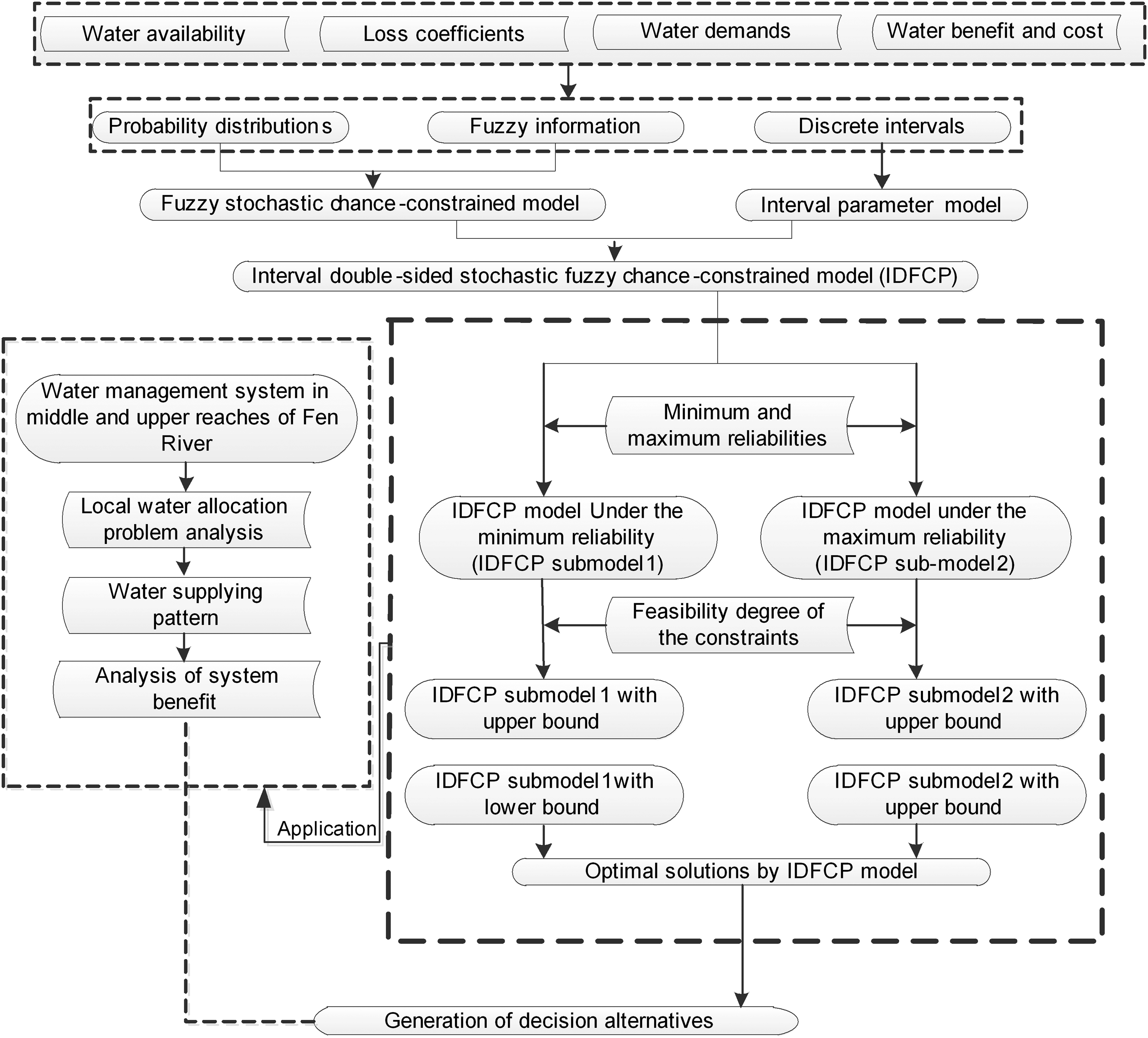
Generally, the proposed IDFCP is capable of handling uncertainties described in both fuzzy and interval formats; meanwhile, more abundant results can be obtained under different α-cut levels at different confidence levels. The general framework of IDFCP is presented in Fig. 1.
General framework of IDFCP. IDFCP, interval double-sided fuzzy chance-constrained programming.
Case Study
Problem statement
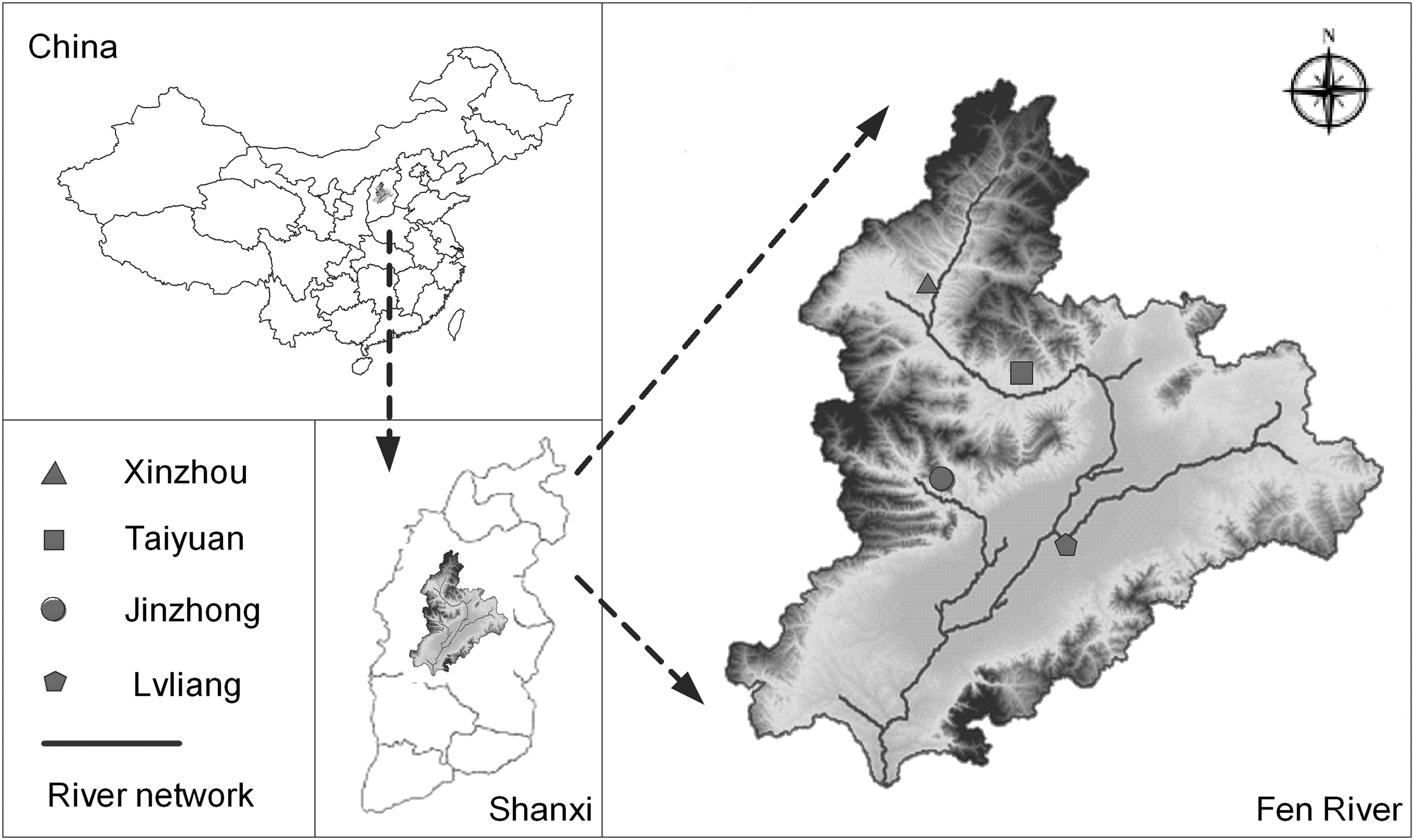
Fen River Basin is located between 35°8′N and 39°8′N, and 110°50′E and 120°40′E in Shanxi province with a draining area of 39,740 km2 (as shown in Fig. 2). Fen River is the second largest tributary of the Yellow River with a length of 713 km; the annual stream flow reaches 1,500 × 109 m3. The basin experiences a temperate monsoon climate. Annual precipitation is 456.0 mm. The main rainfall season is from May to September, with a flooding season from July to August. The annual average temperature in this region is 9.8°C with a range of 6.0–13.0°C (Zhu et al., 2016).
The study area.
The middle and upper reaches of Fen River cover four urban regions, including Xinzhou (XZ), Taiyuan (TY), Lvliang (LL), and Jinzhong (JZ). Municipal administration, industry, agriculture, and ecology are the main water consumers in these cities. In recent years, the rapid development of industrialization and agricultural reclamation has largely squeezed ecological water, causing serious ecological degradation. The ground water table shrinks and surface water reduces heavily due to climate change and human activities. Besides, as one of the important water sources, reclaimed water utilization ration in this region is less than 25%, resulting in low efficiency of water use. The severe competition between water demand and water supply has further aggravated water shortages in this region. Moreover, the complexities and uncertainties in the water resources management system make water allocation more challenging. Therefore, it is desirable to develop a more robust method for water allocation in the Fen River Basin for decision makers in face of multiple sources, multiple users, and multiple regions.
In this study, the data include economic data, water resources data, and pollution data, which were obtained from the statistic year books (2010–2016) of Shanxi Province, government reports, and related researches. Table 1 presents the water demands of different sectors in study area, which are expressed as intervals. Table 2 shows the water availabilities of surface water and groundwater in the middle and upper reaches of Fen River Basin. The amount of available water can be presented as fuzzy interval. Table 3 shows the economic data, including cost of water supply and profit when water demand is satisfied, which are mainly obtained from government reports and local policy surveys. Table 4 presents the loss coefficients of supplied water from different sources, which can be expressed as fuzzy sets.
Water Demands That Are Expressed as Intervals (106m3)
Water Availabilities That Are Presented as Fuzzy Distribution Information (106m3)
Surface water
Ground water
Risk levels
Membership grades of fuzzy variables
k = 1
k = 2
k = 3
k = 1
k = 2
k = 3
Under the minimum credibility
p = 0.01
α = 0.2
[485.5, 625.2]
[491.2, 572.7]
[399.4, 516.0]
[530.1, 661.9]
[470.4, 558.0]
[424.6, 507.1]
α = 0.4
[479.7, 616.8]
[493.5, 563.6]
[392.4, 507.0]
[525.9, 656.0]
[465.7, 553.3]
[419.6, 501.8]
α = 0.6
[473.8, 608.2]
[475.7, 554.6]
[385.4, 497.9]
[521.8, 650.3]
[461.0, 548.5]
[414.5, 496.4]
α = 0.8
[468.0, 599.7]
[468.0, 545.6]
[378.4, 488.9]
[517.6, 644.3]
[456.4, 543.8]
[409.5, 491.1]
p = 0.05
α = 0.2
[521.6, 700.0]
[559.4, 648.1]
[456.3, 590.5]
[567.0, 710.4]
[507.3, 597.5]
[467.0, 550.5]
α = 0.4
[514.1, 683.5]
[544.3, 631.5]
[443.8, 574.1]
[558.8, 699.7]
[498.0, 588.8]
[457.6, 541.0]
α = 0.6
[506.5, 666.9]
[529.2, 614.9]
[431.3, 557.8]
[550.6, 689.1]
[488.6, 580.2]
[448.3, 531.4]
α = 0.8
[499.0, 650.3]
[514.1, 598.3]
[418.8, 541.4]
[542.4, 678.4]
[479.3, 571.5]
[439.0, 521.9]
p = 0.10
α = 0.2
[660.2, 759.3]
[618.9, 692.9]
[597.7, 681.4]
[669.4, 760.2]
[607.3, 681.2]
[599.3, 672.0]
α = 0.4
[627.5, 748.7]
[607.8, 685.9]
[565.5, 662.8]
[645.9, 750.4]
[584.6, 662.5]
[568.5, 644.0]
α = 0.6
[594.7, 737.9]
[596.7, 678.8]
[533.2, 644.1]
[622.3, 740.6]
[562.0, 643.7]
[537.8, 616.0]
α = 0.8
[562.0, 727.2]
[585.7, 671.7]
[501.0, 625.5]
[598.8, 730.8]
[539.3, 625.0]
[507.0, 588.0]
Under the maximum credibility
p = 0.01
α = 0.2
[432.6, 546.6]
[420.9, 493.7]
[338.9, 437.0]
[492.3, 609.3]
[430.5, 516.6]
[380.8, 460.0]
α = 0.4
[440.0, 557.8]
[430.7, 504.4]
[347.0, 447.7]
[497.6, 616.6]
[435.8, 522.2]
[386.7, 466.5]
α = 0.6
[447.6, 568.9]
[440.6, 515.1]
[355.1, 458.4]
[502.9, 623.8]
[441.1, 527.8]
[392.6, 472.9]
α = 0.8
[454.7, 580.0]
[450.4, 525.8]
[363.3, 469.1]
[508.2, 631.1]
[446.4, 533.4]
[398.5, 479.4]
p = 0.05
α = 0.2
[468.0, 599.7]
[468.0, 545.6]
[378.4, 488.9]
[517.6, 644.3]
[456.4, 543.8]
[409.5, 491.1]
α = 0.4
[473.8, 608.1]
[475.7, 554.6]
[385.4, 497.9]
[521.8, 650.2]
[461.0, 548.5]
[414.5, 496.4]
α = 0.6
[479.7, 616.7]
[483.5, 563.6]
[392.4, 506.9]
[525.9, 656.0]
[465.7, 553.3]
[419.6, 501.8]
α = 0.8
[485.5, 625.2]
[491.2, 572.7]
[399.4, 516.0]
[530.1, 661.9]
[470.4, 558.0]
[424.6, 507.1]
p = 0.10
α = 0.2
[499.0, 650.3]
[514.1, 598.3]
[418.8, 541.4]
[542.4, 678.4]
[484.3, 571.4]
[439.0, 521.9]
α = 0.4
[506.5, 666.9]
[529.2, 614.9]
[431.3, 557.8]
[550.6, 689.1]
[493.7, 580.2]
[448.3, 531.4]
α = 0.6
[514.1, 683.5]
[544.3, 631.5]
[443.8, 574.1]
[558.8, 699.7]
[503.0, 588.8]
[457.6, 541.0]
α = 0.8
[521.6, 700.0]
[559.4, 648.1]
[456.3, 590.5]
[567.0, 710.4]
[512.3, 597.5]
[467.0, 550.5]
Economic Data
User sectors
Sources
Time period (k)
Municipal
Industrial
Agricultural
Ecological
Costs of supplying water from sources to users ($/m3)
Surface water
k = 1
[0.64, 0.70]
[0.50, 0.62]
[0.53, 0.63]
[0.46, 0.54]
k = 2
[0.72, 0.80]
[0.58, 0.68]
[0.61, 0.70]
[0.55, 0.65]
k = 3
[0.86, 0.93]
[0.64, 0.82]
[0.77, 0.85]
[0.64, 0.75]
Ground water
k = 1
[0.46, 0.58]
[0.43, 0.55]
[0.40, 0.52]
[0.40, 0.48]
k = 2
[0.56, 0.67]
[0.53, 0.65]
[0.50, 0.62]
[0.50, 0.59]
k = 3
[0.64, 0.76]
[0.61, 0.73]
[0.58, 0.72]
[0.58, 0.66]
Reclaimed water
k = 1
[2.25, 2.54]
[0.40, 0.55]
[1.72, 1.98]
[0.50, 0.60]
k = 2
[2.51, 2.85]
[0.50, 0.65]
[1.87, 2.20]
[0.60, 0.68]
k = 3
[2.79, 3.20]
[0.60, 0.75]
[2.09, 2.32]
[0.70, 0.82]
Net benefit when water demand is satisfied ($/m3)
k = 1
[8.00, 10.00]
[5.00, 6.50]
[0.70, 0.85]
[1.50, 2.00]
k = 2
[9.00, 11.00]
[5.50, 7.00]
[0.80, 0.95]
[2.50, 3.00]
k = 3
[10.00, 12.00]
[6.00, 7.50]
[0.90, 1.00]
[3.50, 4.00]
Loss Coefficients of Supplied Water from Different Sources That Are Presented as Fuzzy Variables
Period (k)
Sources
Membership grades of fuzzy variables
k = 1
k = 2
k = 3
Surface water
α = 0.2
[0.11, 0.19]
[0.104, 0.144]
[0.084, 0.104]
α = 0.4
[0.12, 0.18]
[0.108, 0.138]
[0.088, 0.108]
α = 0.6
[0.13, 0.17]
[0.112, 0.132]
[0.092, 0.112]
α = 0.8
[0.14, 0.16]
[0.116, 0.126]
[0.096, 0.116]
Groundwater
α = 0.2
[0.104, 0.144]
[0.084, 0.104]
[0.056, 0.084]
α = 0.4
[0.108, 0.138]
[0.088, 0.108]
[0.062, 0.088]
α = 0.6
[0.112, 0.132]
[0.092, 0.112]
[0.068, 0.092]
α = 0.8
[0.116, 0.126]
[0.096, 0.116]
[0.074, 0.096]
Reclaimed water
0.085
0.08
0.075
Modeling formulation
The problem under consideration is how to effectively allocate the limited water to four sectors in four regions along the middle and upper reaches of Fen River Basin. A 9-year planning horizon is considered, with the first planning period being from 2017 to 2019, the second from 2020 to 2022, and the third from 2023 to 2025. In this study, water availabilities of surface and groundwater resources and loss coefficient exist as fuzzy sets, which may result in double-sided ambiguity. Net benefit, net cost, water demands, and other parameters are given as interval values. Thus, the IDFCP method is suitable for Fen River water resources management under mixed uncertainties. The IDFCP model can be formulated as follows:
\documentclass{aastex}\usepackage{amsbsy}\usepackage{amsfonts}\usepackage{amssymb}\usepackage{bm}\usepackage{mathrsfs}\usepackage{pifont}\usepackage{stmaryrd}\usepackage{textcomp}\usepackage{portland, xspace}\usepackage{amsmath, amsxtra}\usepackage{upgreek}\pagestyle{empty}\DeclareMathSizes{10}{9}{7}{6}\begin{document}
\begin{align*}
\begin{split} Max{f^ { \pm} } & = \mathop \sum \limits_{i = 1}^4 { \mathop \sum \limits_{j = 1}^4 { \mathop \sum \limits_{k = 1}^3 {P{T_{ik}}^ { \pm} d{f_k}^ { \pm} \left( {S{W_{ijk}}^ { \pm} + G{W_{ijk}}^ { \pm} + R{W_{ijk}}^ { \pm} } \right) } } } \\ & - d{f_k}^ { \pm} \mathop \sum \limits_{i = 1}^4 { \mathop \sum \limits_{j = 1}^4 { \mathop \sum \limits_{k = 1}^3 {C{S_{ijk}}^ { \pm} S{W_{ijk}}^ { \pm} } } } \\ & - d{f_k}^ { \pm} \mathop \sum \limits_{i = 1}^4 { \mathop \sum \limits_{j = 1}^4 { \mathop \sum \limits_{k = 1}^3 {C{G_{ijk}}^ { \pm} G{W_{ijk}}^ { \pm} } } } \\ & - d{f_k}^ { \pm} \mathop \sum \limits_{i = 1}^4 { \mathop \sum \limits_{j = 1}^4 { \mathop \sum \limits_{k = 1}^3 {C{R_{ijk}}^ { \pm} R{W_{ijk}}^ { \pm} } } } ,\end{split}
\tag{14a}
\end{align*}
\end{document}
subject to:
1. Water availability constraints of surface water:
The detail nomenclatures for the variables and parameters are provided in Appendix C. When solving the above submodels, reasonable solutions for optimal effluent trading scheme can be obtained. The framework of the proposed IDFCP is shown in Fig. 1. Each technique of the modeling system has a unique contribution in enhancing the model's capability in handling uncertainties and complexities in water resources management system. The solution algorithm can be summarized by using the following steps:
Step 1: Formulate IDFCP model (14).
Step 2: Transform the IDFCP model into two submodels corresponding to the minimum and maximum credibilities.
Step 3: Transform the interval submodels under the minimum and maximum credibilities into upper and lower bound submodels, where the submodels corresponding to \documentclass{aastex}\usepackage{amsbsy}\usepackage{amsfonts}\usepackage{amssymb}\usepackage{bm}\usepackage{mathrsfs}\usepackage{pifont}\usepackage{stmaryrd}\usepackage{textcomp}\usepackage{portland, xspace}\usepackage{amsmath, amsxtra}\usepackage{upgreek}\pagestyle{empty}\DeclareMathSizes{10}{9}{7}{6}\begin{document}
$${f^ + }$$
\end{document} are first desired since the objective is to maximize \documentclass{aastex}\usepackage{amsbsy}\usepackage{amsfonts}\usepackage{amssymb}\usepackage{bm}\usepackage{mathrsfs}\usepackage{pifont}\usepackage{stmaryrd}\usepackage{textcomp}\usepackage{portland, xspace}\usepackage{amsmath, amsxtra}\usepackage{upgreek}\pagestyle{empty}\DeclareMathSizes{10}{9}{7}{6}\begin{document}
$${f^ { \pm} }$$
\end{document}.
Step 4: Solve the submodels under different scenarios and obtain the solutions of \documentclass{aastex}\usepackage{amsbsy}\usepackage{amsfonts}\usepackage{amssymb}\usepackage{bm}\usepackage{mathrsfs}\usepackage{pifont}\usepackage{stmaryrd}\usepackage{textcomp}\usepackage{portland, xspace}\usepackage{amsmath, amsxtra}\usepackage{upgreek}\pagestyle{empty}\DeclareMathSizes{10}{9}{7}{6}\begin{document}
$$x_{opt}^ +$$
\end{document} and \documentclass{aastex}\usepackage{amsbsy}\usepackage{amsfonts}\usepackage{amssymb}\usepackage{bm}\usepackage{mathrsfs}\usepackage{pifont}\usepackage{stmaryrd}\usepackage{textcomp}\usepackage{portland, xspace}\usepackage{amsmath, amsxtra}\usepackage{upgreek}\pagestyle{empty}\DeclareMathSizes{10}{9}{7}{6}\begin{document}
$$f_{opt}^ +$$
\end{document}.
Step 5: Formulate and solve the \documentclass{aastex}\usepackage{amsbsy}\usepackage{amsfonts}\usepackage{amssymb}\usepackage{bm}\usepackage{mathrsfs}\usepackage{pifont}\usepackage{stmaryrd}\usepackage{textcomp}\usepackage{portland, xspace}\usepackage{amsmath, amsxtra}\usepackage{upgreek}\pagestyle{empty}\DeclareMathSizes{10}{9}{7}{6}\begin{document}
$${f^ - }$$
\end{document} submodels by following the same interactive procedure as that in \documentclass{aastex}\usepackage{amsbsy}\usepackage{amsfonts}\usepackage{amssymb}\usepackage{bm}\usepackage{mathrsfs}\usepackage{pifont}\usepackage{stmaryrd}\usepackage{textcomp}\usepackage{portland, xspace}\usepackage{amsmath, amsxtra}\usepackage{upgreek}\pagestyle{empty}\DeclareMathSizes{10}{9}{7}{6}\begin{document}
$${f^ + }$$
\end{document} submodels.
Step 6: Obtain decision alternatives under different p levels, α-cut levels, and different credibilities by considering the solutions from four submodels.
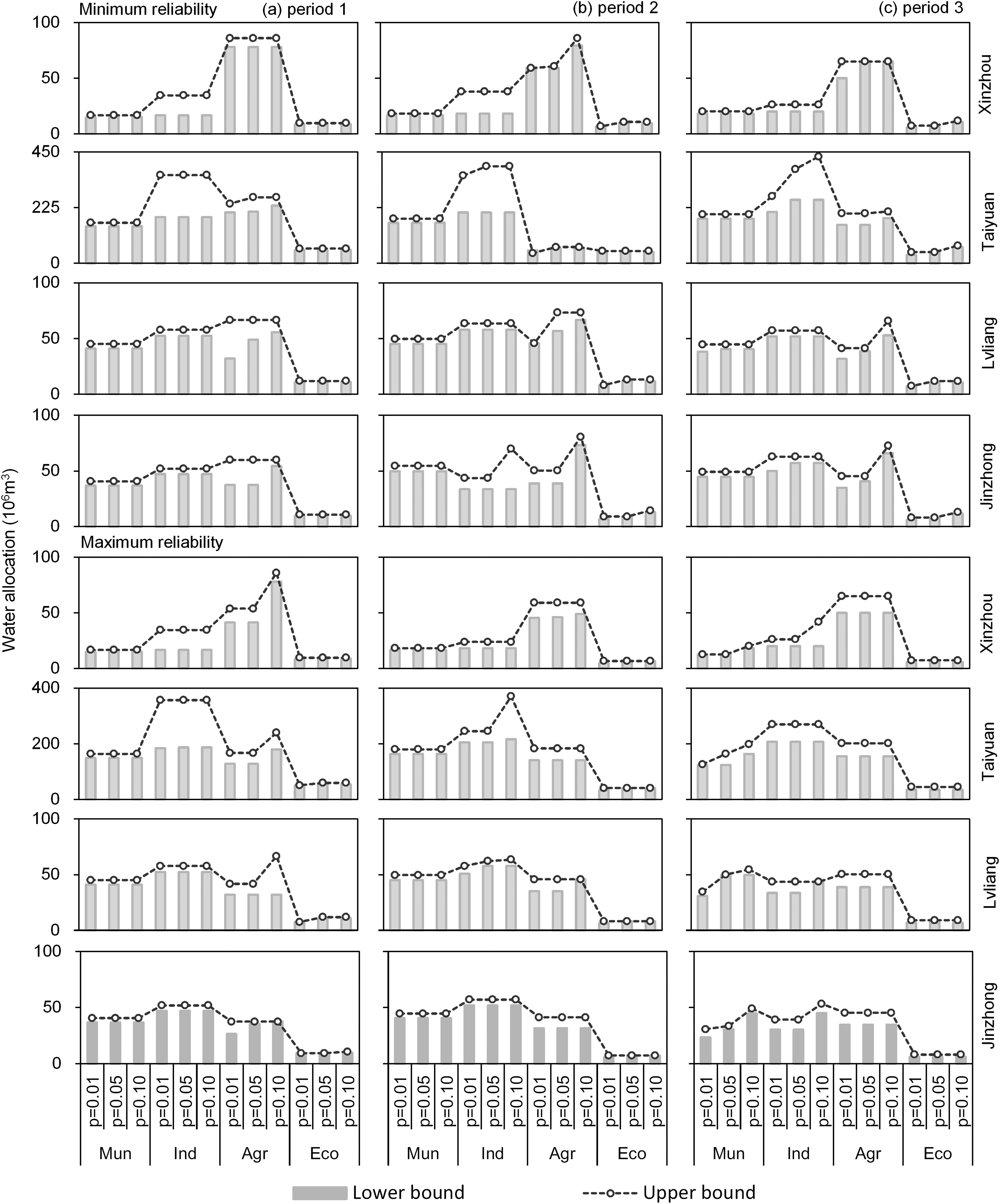
In this study, four utilization ratios of reclaimed water (η), three p levels, four α-cut levels, and two credibilities were examined, leading to 98 scenarios. Figures 3 and 4 present the solutions of water allocation under all scenarios, implying that different combinative considerations on the uncertain inputs would lead to varied water allocation plans. In detail, the amount of water allocation would increase with η and p levels. The result also indicates that under the minimum credibility, the amount of allocated water would decrease with the increasing of α-cut level; under the maximum credibility, the amount would increase with the increasing of α-cut level. Besides, promoting the utilization ratio of reclaimed water would contribute to an increased amount of allocated water. It is also found that in the scenario of η = 60%, p = 0.10, and α = 0.2 with the minimum credibility, the total water allocation amount to the basin reaches the highest (i.e., [1048.7,1336.9], [1169.6, 1470.6], and [1286.5, 1617.6] × 106 m3 from period 1 to 3), while the lowest (i.e., [1016.6, 1336.9], [1134.3, 1444.6], and [1116.8, 1443.0] × 106 m3 from period 1 to 3) is under the scenario of η = 30%, p = 0.01, and α = 0.8 with the maximum credibility. It is indicated that the water allocation is scenario based and greatly influenced by the decision makers' preferences.
Water allocation obtained under the minimum credibility (106 m3).
Water allocation obtained under the maximum credibility (106 m3) [(a) period 1; (b) period 2 and (c) period 3].
Figure 5 shows the optimized water allocation volumes to the municipal, industrial, and agricultural sectors under different p levels with both credibilities. The results show that the amount of allocated water to users would increase with p level. In detail, in period 1, when η = 30% and α = 0.2 (under the maximum credibility), the optimized water allocation plans for industrial sector in TY would increase from [128.1, 166.6] × 106 m3 to [179.7, 239.8] × 106 m3 when p increases from 0.01 to 0.10. Similar change trends could be found in both periods 2 and 3. This is due to the fact that an increased p level means a raised risk in violating the water availability constraint, which would lead to decreased strictness for the constraint and contribute to more water availabilities. Although decisions at a higher p level would result in a higher amount of water allocation, the violation risk of constraints and system failure would be raised; in comparison, a lower p level would correspond to a lower amount of water allocation but with an increased confidence level in fulfilling the system constraints.
Water allocation plans for different users at varying p levels (η = 30%) (106 m3). Agr, agricultural sector; Eco, ecological sector; Ind, industrial sector; Mun, municipal sector.
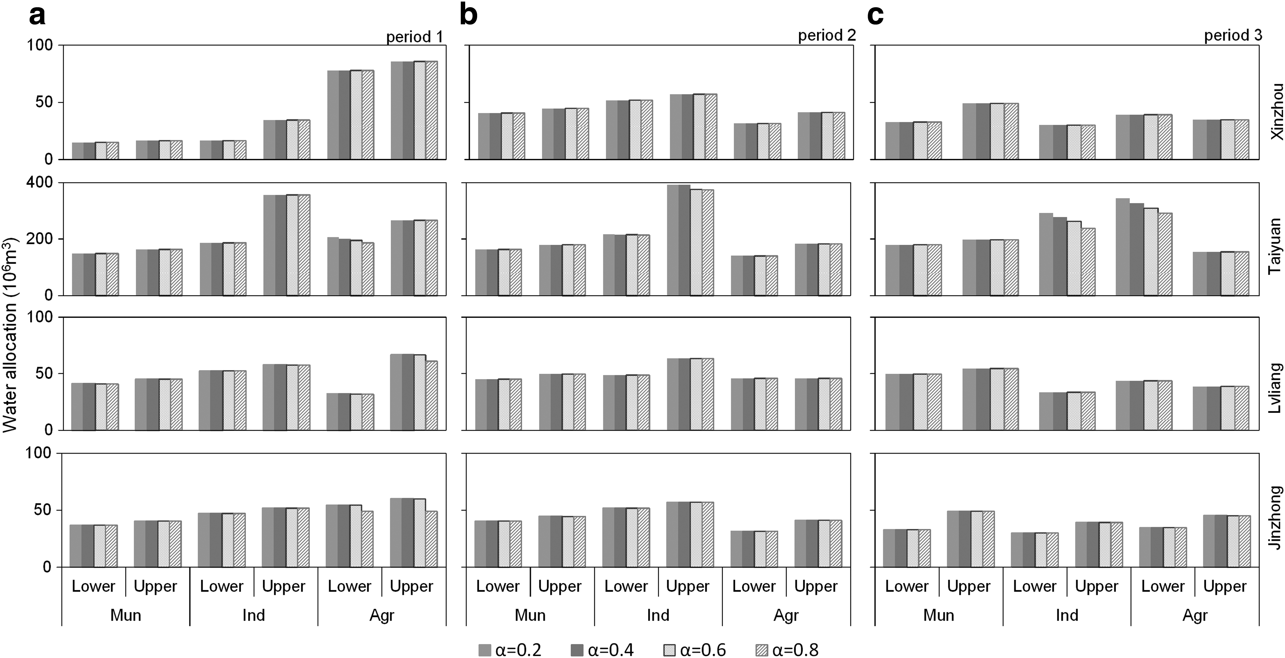
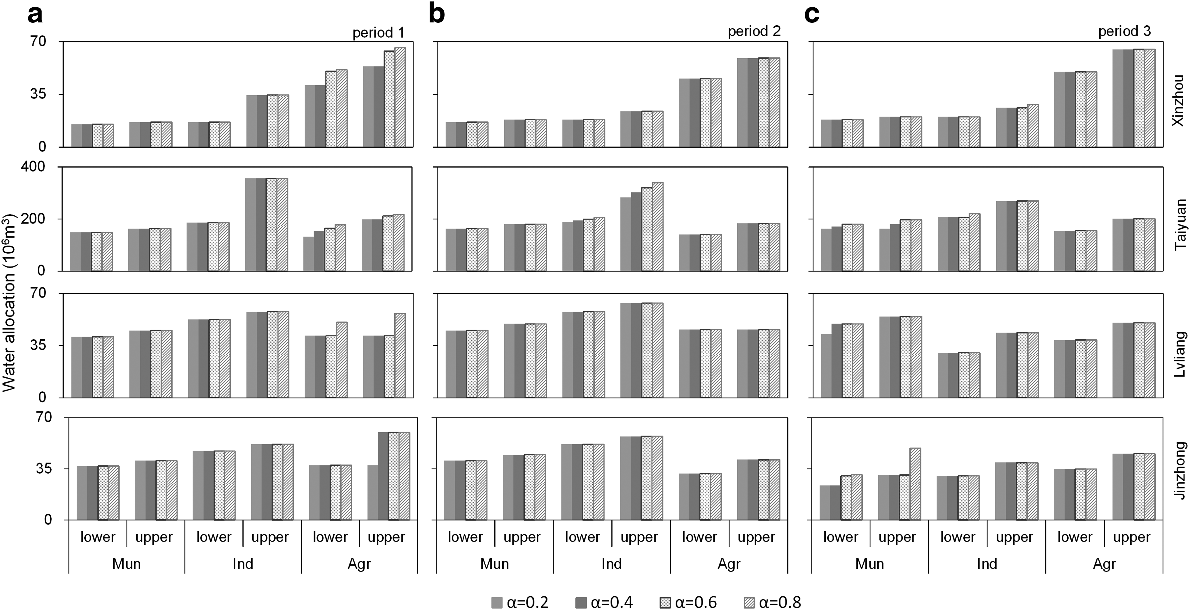
Figures 6 and 7 present water allocation plans for different users under different α-cut levels with minimum and maximum credibilities, respectively. The results indicate that different α-cut levels would lead to varied solutions for water allocation. Under the maximum credibility, an increased α-cut level would correspond to increment in water allocation amount; contrarily, increased α-cut level has a negative impact on water allocation under the minimum credibility. For example, in period 2, under the maximum credibility, the water allocation plans for industrial sector in TY would promote from [190.1, 283.9] × 106 m3 (p = 0.01, α = 0.2) to [205.1, 339. 6] × 106 m3 (p = 0.01, α = 0.8); under the minimum credibility, the amount of water allocation for industrial sector in TY would decrease from [216.2, 391.9] × 106 m3 to [214.49, 374.4] × 106 m3. This is because different α-cut levels are associated with varied system conditions (i.e., loss coefficient and water availability); the interval for fuzzy variables is wider under a lower α-cut level but narrower under a higher α-cut level. Namely, an increased α-cut level will result in a lower loss coefficient and higher water availability under the maximum credibility. Results also show that water deficits would occur in industrial and agricultural sectors if the available water does not meet the water demands. Meanwhile, when the water demand of industrial sector is satisfied, the amount of water allocation for agricultural sector would increase because the benefit from the industrial sector is higher than that from the agricultural sector. Thus, the IDFCP approach provides more useful information for decision makers regarding the trade-off between the amount of water allocation and the probability for satisfying the constraints.
Water allocation for different users under different α-cut levels with the minimum credibility (η = 40%, p = 0.01) (106 m3) [(a) period 1; (b) period 2 and (c) period 3].
Water allocation for different users under different α-cut levels with the maximum credibility (η = 40%, p = 0.01) (106 m3) [(a) period 1; (b) period 2 and (c) period 3].
Table 5 shows the total amount of allocated water under different credibilities. Results indicate that the amount of water allocation under the minimum credibility is higher than that under the maximum credibility. For example, in period 1, when p = 0.01 and α = 0.2, the total amount of allocated water would be [1016.7, 1336.8] × 106 m3 and [930.8, 1239.0] × 106 m3 under minimum and maximum credibilities, respectively; this can be attributed to the minimum credibility corresponding to a lower loss coefficient and higher water availability than the maximum credibility. Generally, the minimum credibility would cause smaller water resources pressure but lower stability of the system.
Total Amount of Allocated Water Under Different Credibilities (η = 50%) (106m3)
Time periods (k)
p
α-cut
Credibility
k = 1
k = 2
k = 3
0.01
0.2
Min
[1016.7, 1336.8]
[993.3, 1306.7]
[1045.1, 1289.7]
Max
[930.8, 1239.0]
[939.4, 1167.7]
[925.6, 1144.9]
0.4
Min
[1008.3, 1336.8]
[983.4, 1290.4]
[1030.3, 1272.0]
Max
[945.0, 1261.6]
[939.7, 1186.1]
[940.7, 1163.4]
0.6
Min
[1002.2, 1336.8]
[967.6, 1274.3]
[1015.6, 1254.3]
Max
[965.6, 1284.4]
[940.2, 1204.6]
[955.9, 1182.0]
0.8
Min
[994.2, 1336.8]
[959.7, 1228.2]
[1001.1, 1236.9]
Max
[978.6, 1307.6]
[959.7, 1258.2]
[971.2, 1200.7]
0.05
0.2
Min
[1021.1, 1336.8]
[1095.0, 1411.4]
[1072.1, 1399.6]
Max
[962.3, 1254.8]
[958.9, 1182.0]
[987.2, 1160.4]
0.4
Min
[1016.1, 1336.8]
[1067.6, 1384.3]
[1052.0, 1370.6]
Max
[987.2, 1336.8]
[957.1, 1253.8]
[1000.7, 1235.9]
0.6
Min
[1007.6, 1336.8]
[1040.4, 1357.4]
[1048.6, 1341.9]
Max
[994.6, 1336.8]
[966.5, 1270.5]
[1014.3, 1252.3]
0.8
Min
[1003.6, 1336.8]
[1013.4, 1330.7]
[1041.8, 1313.5]
Max
[998.3, 1336.8]
[981.3, 1287.2]
[1028.0, 1268.7]
0.10
0.2
Min
[1048.7, 1336.8]
[1169.6, 1470.6]
[1274.7, 1598.5]
Max
[998.8, 1336.8]
[1003.7, 1308.3]
[1043.1, 1294.9]
0.4
Min
[1036.6, 1336.8]
[1169.6, 1470.6]
[1228.9, 1549.1]
Max
[1005.6, 1336.8]
[1021.1, 1335.2]
[1048.2, 1321.8]
0.6
Min
[1024.6, 1336.8]
[1169.6, 1470.6]
[1177.8, 1500.2]
Max
[1012.8, 1336.8]
[1043.2, 1362.5]
[1050.4, 1348.9]
0.8
Min
[1020.6, 1336.8]
[1152.9, 1445.3]
[1127.2, 1451.8]
Max
[1016.2, 1336.8]
[1079.6, 1390.0]
[1059.1, 1376.3]
Figure 8 presents water allocation under a range of utilization ratios of reclaimed water under the maximum credibility. It is shown that in period 2, when p = 0.05 and α = 0.4, the water allocation plans for industrial sector in XZ would be [18.3, 23.8] × 106 m3 and [18.3, 38.0] × 106 m3 when η = 30% and 60%, respectively. The amount of water allocation for agricultural sector in JZ would be [31.7, 41.2] × 106 m3 and [46.2, 65.9] × 106 m3. The results indicate that promotion of reclaimed water utilization would help increase water allocation volumes to industrial and agricultural sectors. This is because the supplement of reclaimed water would satisfy the industrial and ecological water demands, leading more surface water and ground water to be assigned to the agricultural sector, and finally releasing water shortage. Generally, effective measures should be taken to improve the reclaimed water utilization ratio for enhancing the sustainable development of water resources system.
Water allocation for different users under different utilization ratios of reclaimed water (p = 0.05, α = 0.4) (106 m3).
Table 6 presents the solutions of system benefit under all scenarios. Results indicate that system benefits would increase with p and η levels, decrease with α-cut level under the minimum credibility, and increase with α-cut level under maximum credibility. For example, under the minimum credibility, when η = 30%, p = 0.01, the system benefits would be $ [8.54, 15.90] × 109 and $ [8.32, 15.28] × 109 under α = 0.2, and 0.8, respectively; when η = 30%, p = 0.10, the system benefits would be $ [8.89, 17.37] × 109 and $ [8.81, 17.01] × 109 under α = 0.2, and 0.8, respectively. It is due to the fact that, when p level increases, the risk of violating the water availability constraint increased, which would lead to a higher amount of water allocation, but with a lower confidence level. An increased utilization ratio of reclaimed water could enhance system benefits due to increased water supply. System benefit is highly scenario dependent. Decision makers would like to select water allocation patterns that could bring higher benefits; however, higher benefits usually correspond to higher system violating risks. The system benefit analysis provides decision makers trade-offs between system benefits and water sustainability, which could help gain insight into the characteristics and risks of the water resources management system.
System Benefit Under All Scenarios ($109)
Minimum credibility
Maximum credibility
η
η
p
α-cut
30%
40%
50%
60%
30%
40%
50%
60%
0.01
0.2
[8.54, 15.90]
[8.71, 16.48]
[8.77, 16.87]
[8.78, 17.22]
[7.83, 14.00]
[8.22, 14.87]
[8.47, 15.67]
[8.65, 16.31]
0.4
[8.49, 15.72]
[8.65, 16.36]
[8.77, 16.77]
[8.78, 17.12]
[7.95, 14.28]
[8.31, 15.12]
[8.52, 15.86]
[8.71, 16.49]
0.6
[8.42, 15.51]
[8.60, 16.18]
[8.77, 16.68]
[8.78, 17.03]
[8.08, 14.53]
[8.39, 15.37]
[8.57, 16.06]
[8.74, 16.62]
0.8
[8.32, 15.58]
[8.58, 16.00]
[8.75, 16.56]
[8.78, 16.94]
[8.14, 14.79]
[8.45, 15.62]
[8.63, 16.26]
[8.78, 16.65]
0.05
0.2
[8.80, 16.74]
[8.81, 17.09]
[8.87, 17.34]
[8.88, 17.38]
[8.17, 14.23]
[8.50, 15.07]
[8.70, 15.83]
[8.77, 16.46]
0.4
[8.79, 15.69]
[8.80, 16.94]
[8.83, 17.26]
[8.88, 17.37]
[8.33, 15.24]
[8.58, 15.97]
[8.75, 16.55]
[8.78, 16.93]
0.6
[8.71, 16.40]
[8.79, 16.79]
[8.81, 17.14]
[8.87, 17.35]
[8.41, 15.47]
[8.62, 16.15]
[8.77, 16.66]
[8.78, 17.02]
0.8
[8.61, 16.15]
[8.77, 16.64]
[8.78, 16.99]
[8.83, 17.29]
[8.48, 15.68]
[8.64, 16.32]
[8.77, 16.75]
[8.78, 17.11]
0.10
0.2
[8.89, 17.37]
[8.90, 17.41]
[8.91, 17.43]
[8.92, 17.44]
[8.56, 15.93]
[8.73, 16.51]
[8.78, 16.89]
[8.79, 17.23]
0.4
[8.88, 17.34]
[8.89, 17.38]
[8.90, 17.41]
[8.91, 17.44]
[8.63, 16.22]
[8.78, 16.68]
[8.79, 17.03]
[8.84, 17.31]
0.6
[8.83, 17.25]
[8.88, 17.36]
[8.90, 17.39]
[8.90, 17.42]
[8.73, 16.44]
[8.80, 16.83]
[8.81, 17.18]
[8.87, 17.35]
0.8
[8.81, 17.01]
[8.86, 17.30]
[8.89, 17.39]
[8.90, 17.40]
[8.79, 16.22]
[8.81, 16.97]
[8.84, 17.28]
[8.88, 17.37]
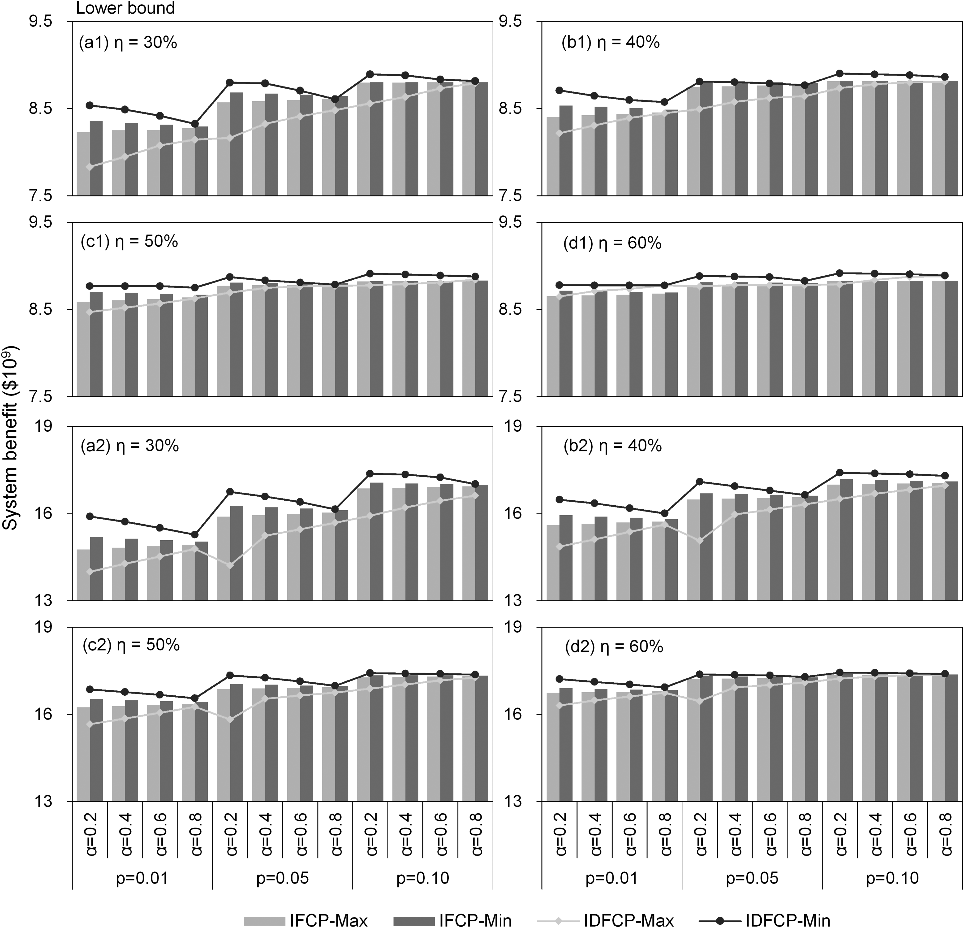
The study problem can turn into an interval single-sided fuzzy chance-constrained programming (ISFCP) by predigesting parameters on the right side of the constraints in a nonfuzzy space. Figure 9 presents the solutions obtained from IDFCP and ISFCP. The interval of system benefit between minimum and maximum credibilities from IDFCP is wider than the interval obtained from ISFCP. For example, when η = 30%, p = 0.01, and α = 0.2, the upper bound of system benefits obtained from IDFCP would be $ [14.00, 15.90] × 109; the upper bound of system benefits obtained from ISFCP would be $ [14.77, 15.20] × 109. This indicates that IDFCP could provide more relaxed decision space for decision makers. In fact, in water resources management system, the amount of available water as well as loss coefficients may exist as fuzzy sets, and thus, the ISFCP may encounter difficulty for solving the fuzzy sets on both sides of the constraints. In comparison, IDFCP can effectively deal with the issues through introducing the double-sided FMP method and provide a wider decision space for managers.
System benefits from IDFCP and interval single-sided fuzzy chance-constrained programming (ISFCP) ($109) [Max means maximum credibility and Min means minimum credibility].
Conclusions
In this study, the IDFCP model has been developed for water resources management. IDFCP improves on the existing CCP, FMP, and IPP. IDFCP has the following advantages such as (1) tackling uncertainties expressed as probability distributions, fuzzy sets, and intervals, leading to enhanced system robustness for uncertainty reflection, (2) it also allows examining risks of system constraint violation at specified confidence levels and provides information on trade-offs and the relationship between objective function value and the specified probability of constraints, (3) handling fuzzy sets on both sides of the constraints, and (4) providing more reliable water resources management alternatives for decision makers.
The IDFCP method has been applied to a real case for planning water resources allocation in the middle and upper reaches of Fen River, China. Results associated with different utilization ratios of reclaimed water, risk levels, α-cut levels, and minimum and maximum credibilities have been generated. Results indicate that (1) the higher risk of violating the water availability constraint corresponds to a higher allocated water level and a higher system benefit; (2) under the maximum credibility, the amount of water allocation and system benefit would increase with the α-cut levels; conversely, they would decline under the minimum credibility with the α-cut levels; (3) the amount of water allocation and system benefit under the minimum credibility is higher than that under the maximum credibility. The results obtained can be useful for generating a series of alternatives under various scenarios and thus can help decision makers to identify desired water resources plan under the uncertainties.
Although the result obtained from IDFCP provides desirable water allocation patterns under different scenarios, water shortage still exists in the study area. The industry would require the most water resources in this area and the demand for water would increase due to its high-speed development. Therefore, effective water saving techniques for the industry user should be adopted for decreasing its water demand and the related technology should be improved for promoting the utilization ratio of reclaimed water. Municipal and industrial sectors would own the priority of water allocation due to their higher profits. Thus, it is desired to make a balance between different water users according to their demands. Besides, in the real-world water resources management problems, more natural factors should be taken into account such as the interaction between surface water and groundwater, while multiobjectives (e.g., efficiency of water use and food safety) should attract attention in future research works.
Footnotes
Acknowledgments
This research was supported by the Natural Science Foundation of China (51779008) and the National Key Research Development Program of China (2016 YFA 0601502 and 2016 YFC0502803). The authors deeply appreciate the editors and the anonymous reviewers for their insightful comments and helpful suggestions.
Author Disclosure Statement
No competing financial interests exist.
Appendix A. Proof for Relation (3b) to Crisp Relations
Appendix B. Transformation of Interval Programming into Lower and Upper Bound Submodels
An interval parameter programming model can be written as follows (Li et al., 2010):
where \documentclass{aastex}\usepackage{amsbsy}\usepackage{amsfonts}\usepackage{amssymb}\usepackage{bm}\usepackage{mathrsfs}\usepackage{pifont}\usepackage{stmaryrd}\usepackage{textcomp}\usepackage{portland, xspace}\usepackage{amsmath, amsxtra}\usepackage{upgreek}\pagestyle{empty}\DeclareMathSizes{10}{9}{7}{6}\begin{document}
$$c_j^ \pm$$
\end{document}, \documentclass{aastex}\usepackage{amsbsy}\usepackage{amsfonts}\usepackage{amssymb}\usepackage{bm}\usepackage{mathrsfs}\usepackage{pifont}\usepackage{stmaryrd}\usepackage{textcomp}\usepackage{portland, xspace}\usepackage{amsmath, amsxtra}\usepackage{upgreek}\pagestyle{empty}\DeclareMathSizes{10}{9}{7}{6}\begin{document}
$$a_{ij}^ \pm$$
\end{document}, and \documentclass{aastex}\usepackage{amsbsy}\usepackage{amsfonts}\usepackage{amssymb}\usepackage{bm}\usepackage{mathrsfs}\usepackage{pifont}\usepackage{stmaryrd}\usepackage{textcomp}\usepackage{portland, xspace}\usepackage{amsmath, amsxtra}\usepackage{upgreek}\pagestyle{empty}\DeclareMathSizes{10}{9}{7}{6}\begin{document}
$$b_i^ \pm$$
\end{document} from sets of interval values with deterministic lower and upper bounds; the “−” and “+” superscripts represent the lower and upper bounds of parameters/variables, respectively. An interactive solution algorithm was proposed by Huang et al. (1992) to solve the above problem through analyses of the inter-relationships between the parameters and the variables and between the objective function and the constraints. Therefore, when the objective is due to be maximized, a submodel corresponding to \documentclass{aastex}\usepackage{amsbsy}\usepackage{amsfonts}\usepackage{amssymb}\usepackage{bm}\usepackage{mathrsfs}\usepackage{pifont}\usepackage{stmaryrd}\usepackage{textcomp}\usepackage{portland, xspace}\usepackage{amsmath, amsxtra}\usepackage{upgreek}\pagestyle{empty}\DeclareMathSizes{10}{9}{7}{6}\begin{document}
$${f^ \pm }$$
\end{document} can be formulated as follows (assume that \documentclass{aastex}\usepackage{amsbsy}\usepackage{amsfonts}\usepackage{amssymb}\usepackage{bm}\usepackage{mathrsfs}\usepackage{pifont}\usepackage{stmaryrd}\usepackage{textcomp}\usepackage{portland, xspace}\usepackage{amsmath, amsxtra}\usepackage{upgreek}\pagestyle{empty}\DeclareMathSizes{10}{9}{7}{6}\begin{document}
$$b_i^ \pm \succ 0 ,\ {f^ \pm } \succ 0$$
\end{document}):
Through solving the two submodels, interval solutions for decision variables (\documentclass{aastex}\usepackage{amsbsy}\usepackage{amsfonts}\usepackage{amssymb}\usepackage{bm}\usepackage{mathrsfs}\usepackage{pifont}\usepackage{stmaryrd}\usepackage{textcomp}\usepackage{portland, xspace}\usepackage{amsmath, amsxtra}\usepackage{upgreek}\pagestyle{empty}\DeclareMathSizes{10}{9}{7}{6}\begin{document}
$$x_{jopt}^ \pm$$
\end{document}) and the objective function value (\documentclass{aastex}\usepackage{amsbsy}\usepackage{amsfonts}\usepackage{amssymb}\usepackage{bm}\usepackage{mathrsfs}\usepackage{pifont}\usepackage{stmaryrd}\usepackage{textcomp}\usepackage{portland, xspace}\usepackage{amsmath, amsxtra}\usepackage{upgreek}\pagestyle{empty}\DeclareMathSizes{10}{9}{7}{6}\begin{document}
$$x_{jopt}^ \pm$$
\end{document}) can be obtained as follows:
\documentclass{aastex}\usepackage{amsbsy}\usepackage{amsfonts}\usepackage{amssymb}\usepackage{bm}\usepackage{mathrsfs}\usepackage{pifont}\usepackage{stmaryrd}\usepackage{textcomp}\usepackage{portland, xspace}\usepackage{amsmath, amsxtra}\usepackage{upgreek}\pagestyle{empty}\DeclareMathSizes{10}{9}{7}{6}\begin{document}
$${{{f}}^ { \pm} }$$
\end{document}, system benefit.
p, the risk level of violating the water availability constraint (p = 0.01, 0.05, and 0.10).
α, membership grades of fuzzy variables (α = 0.2, 0.4, 0.6, and 0.8).
\documentclass{aastex}\usepackage{amsbsy}\usepackage{amsfonts}\usepackage{amssymb}\usepackage{bm}\usepackage{mathrsfs}\usepackage{pifont}\usepackage{stmaryrd}\usepackage{textcomp}\usepackage{portland, xspace}\usepackage{amsmath, amsxtra}\usepackage{upgreek}\pagestyle{empty}\DeclareMathSizes{10}{9}{7}{6}\begin{document}
$${ {PT}}_{{ {ik}}}^ { \pm}$$
\end{document}, gross benefit of supplying unit water to user i during the period k.
\documentclass{aastex}\usepackage{amsbsy}\usepackage{amsfonts}\usepackage{amssymb}\usepackage{bm}\usepackage{mathrsfs}\usepackage{pifont}\usepackage{stmaryrd}\usepackage{textcomp}\usepackage{portland, xspace}\usepackage{amsmath, amsxtra}\usepackage{upgreek}\pagestyle{empty}\DeclareMathSizes{10}{9}{7}{6}\begin{document}
$${ {df}}_{ {k}}^ { \pm}$$
\end{document}, cash flow discount coefficient during the period k.
\documentclass{aastex}\usepackage{amsbsy}\usepackage{amsfonts}\usepackage{amssymb}\usepackage{bm}\usepackage{mathrsfs}\usepackage{pifont}\usepackage{stmaryrd}\usepackage{textcomp}\usepackage{portland, xspace}\usepackage{amsmath, amsxtra}\usepackage{upgreek}\pagestyle{empty}\DeclareMathSizes{10}{9}{7}{6}\begin{document}
$$CS_{ijk}^ { \pm}$$
\end{document}, cost of supplying unit water from surface water to user i in the area j during the period k.
\documentclass{aastex}\usepackage{amsbsy}\usepackage{amsfonts}\usepackage{amssymb}\usepackage{bm}\usepackage{mathrsfs}\usepackage{pifont}\usepackage{stmaryrd}\usepackage{textcomp}\usepackage{portland, xspace}\usepackage{amsmath, amsxtra}\usepackage{upgreek}\pagestyle{empty}\DeclareMathSizes{10}{9}{7}{6}\begin{document}
$$CG_{ijk}^ { \pm}$$
\end{document}, cost of supplying unit water from groundwater and reclaimed water to user i in the area j during the period k.
\documentclass{aastex}\usepackage{amsbsy}\usepackage{amsfonts}\usepackage{amssymb}\usepackage{bm}\usepackage{mathrsfs}\usepackage{pifont}\usepackage{stmaryrd}\usepackage{textcomp}\usepackage{portland, xspace}\usepackage{amsmath, amsxtra}\usepackage{upgreek}\pagestyle{empty}\DeclareMathSizes{10}{9}{7}{6}\begin{document}
$$CR_{ijk}^ { \pm}$$
\end{document}, cost of supplying unit water from reclaimed water to user i in the area j during the period k.
\documentclass{aastex}\usepackage{amsbsy}\usepackage{amsfonts}\usepackage{amssymb}\usepackage{bm}\usepackage{mathrsfs}\usepackage{pifont}\usepackage{stmaryrd}\usepackage{textcomp}\usepackage{portland, xspace}\usepackage{amsmath, amsxtra}\usepackage{upgreek}\pagestyle{empty}\DeclareMathSizes{10}{9}{7}{6}\begin{document}
$${{SW}}_{{{ijk}}}^ { \pm}$$
\end{document}, water allocation about surface water resource to the user i in the area j during period k.
\documentclass{aastex}\usepackage{amsbsy}\usepackage{amsfonts}\usepackage{amssymb}\usepackage{bm}\usepackage{mathrsfs}\usepackage{pifont}\usepackage{stmaryrd}\usepackage{textcomp}\usepackage{portland, xspace}\usepackage{amsmath, amsxtra}\usepackage{upgreek}\pagestyle{empty}\DeclareMathSizes{10}{9}{7}{6}\begin{document}
$${{GW}}_{{ {ijk}}}^ { \pm}$$
\end{document}, water allocation about groundwater resource to user i in the area j during period k.
\documentclass{aastex}\usepackage{amsbsy}\usepackage{amsfonts}\usepackage{amssymb}\usepackage{bm}\usepackage{mathrsfs}\usepackage{pifont}\usepackage{stmaryrd}\usepackage{textcomp}\usepackage{portland, xspace}\usepackage{amsmath, amsxtra}\usepackage{upgreek}\pagestyle{empty}\DeclareMathSizes{10}{9}{7}{6}\begin{document}
$${ {RW}}_{{{ijk}}}^ { \pm}$$
\end{document}, water allocation about reclaimed water resource to user i in the area j during period k.
\documentclass{aastex}\usepackage{amsbsy}\usepackage{amsfonts}\usepackage{amssymb}\usepackage{bm}\usepackage{mathrsfs}\usepackage{pifont}\usepackage{stmaryrd}\usepackage{textcomp}\usepackage{portland, xspace}\usepackage{amsmath, amsxtra}\usepackage{upgreek}\pagestyle{empty}\DeclareMathSizes{10}{9}{7}{6}\begin{document}
$$\widetilde{LS}_k$$
\end{document}, loss coefficients in the process of water transportation from surface water to users.
\documentclass{aastex}\usepackage{amsbsy}\usepackage{amsfonts}\usepackage{amssymb}\usepackage{bm}\usepackage{mathrsfs}\usepackage{pifont}\usepackage{stmaryrd}\usepackage{textcomp}\usepackage{portland, xspace}\usepackage{amsmath, amsxtra}\usepackage{upgreek}\pagestyle{empty}\DeclareMathSizes{10}{9}{7}{6}\begin{document}
$${ \widetilde{LG}_k}$$
\end{document}, loss coefficients in the process of water transportation from ground water to users.
\documentclass{aastex}\usepackage{amsbsy}\usepackage{amsfonts}\usepackage{amssymb}\usepackage{bm}\usepackage{mathrsfs}\usepackage{pifont}\usepackage{stmaryrd}\usepackage{textcomp}\usepackage{portland, xspace}\usepackage{amsmath, amsxtra}\usepackage{upgreek}\pagestyle{empty}\DeclareMathSizes{10}{9}{7}{6}\begin{document}
$$L{R_k}$$
\end{document}, loss coefficients in the process of water transportation from reclaimed water to users.
\documentclass{aastex}\usepackage{amsbsy}\usepackage{amsfonts}\usepackage{amssymb}\usepackage{bm}\usepackage{mathrsfs}\usepackage{pifont}\usepackage{stmaryrd}\usepackage{textcomp}\usepackage{portland, xspace}\usepackage{amsmath, amsxtra}\usepackage{upgreek}\pagestyle{empty}\DeclareMathSizes{10}{9}{7}{6}\begin{document}
$$\widetilde{SQ}_k^{ \pm}$$
\end{document}, water availability of surface water resource during period k.
\documentclass{aastex}\usepackage{amsbsy}\usepackage{amsfonts}\usepackage{amssymb}\usepackage{bm}\usepackage{mathrsfs}\usepackage{pifont}\usepackage{stmaryrd}\usepackage{textcomp}\usepackage{portland, xspace}\usepackage{amsmath, amsxtra}\usepackage{upgreek}\pagestyle{empty}\DeclareMathSizes{10}{9}{7}{6}\begin{document}
$$\widetilde{GQ}_k^{ \pm}$$
\end{document}, water availability of groundwater resource during period k.
\documentclass{aastex}\usepackage{amsbsy}\usepackage{amsfonts}\usepackage{amssymb}\usepackage{bm}\usepackage{mathrsfs}\usepackage{pifont}\usepackage{stmaryrd}\usepackage{textcomp}\usepackage{portland, xspace}\usepackage{amsmath, amsxtra}\usepackage{upgreek}\pagestyle{empty}\DeclareMathSizes{10}{9}{7}{6}\begin{document}
$$RQ_k^ { \pm}$$
\end{document}, water availability of reclaimed water during period k.
\documentclass{aastex}\usepackage{amsbsy}\usepackage{amsfonts}\usepackage{amssymb}\usepackage{bm}\usepackage{mathrsfs}\usepackage{pifont}\usepackage{stmaryrd}\usepackage{textcomp}\usepackage{portland, xspace}\usepackage{amsmath, amsxtra}\usepackage{upgreek}\pagestyle{empty}\DeclareMathSizes{10}{9}{7}{6}\begin{document}
$$\eta$$
\end{document}, utilization ratio of wastewater.
\documentclass{aastex}\usepackage{amsbsy}\usepackage{amsfonts}\usepackage{amssymb}\usepackage{bm}\usepackage{mathrsfs}\usepackage{pifont}\usepackage{stmaryrd}\usepackage{textcomp}\usepackage{portland, xspace}\usepackage{amsmath, amsxtra}\usepackage{upgreek}\pagestyle{empty}\DeclareMathSizes{10}{9}{7}{6}\begin{document}
$$XWZ_{ijk \, \max }^ { \pm}$$
\end{document}, highest water demand of user i in the area j during period k.
\documentclass{aastex}\usepackage{amsbsy}\usepackage{amsfonts}\usepackage{amssymb}\usepackage{bm}\usepackage{mathrsfs}\usepackage{pifont}\usepackage{stmaryrd}\usepackage{textcomp}\usepackage{portland, xspace}\usepackage{amsmath, amsxtra}\usepackage{upgreek}\pagestyle{empty}\DeclareMathSizes{10}{9}{7}{6}\begin{document}
$$XW_{ijk \, \min }^ { \pm}$$
\end{document}, lowest water demand of user i in the area j during period k.
Ni, nitrogen element content of the water used by user i.
Ci, chemical oxygen demands content of the water used by user i.
\documentclass{aastex}\usepackage{amsbsy}\usepackage{amsfonts}\usepackage{amssymb}\usepackage{bm}\usepackage{mathrsfs}\usepackage{pifont}\usepackage{stmaryrd}\usepackage{textcomp}\usepackage{portland, xspace}\usepackage{amsmath, amsxtra}\usepackage{upgreek}\pagestyle{empty}\DeclareMathSizes{10}{9}{7}{6}\begin{document}
$$GN_k^ { \pm}$$
\end{document}, maximum allowable total nitrogen emissions during period k.
\documentclass{aastex}\usepackage{amsbsy}\usepackage{amsfonts}\usepackage{amssymb}\usepackage{bm}\usepackage{mathrsfs}\usepackage{pifont}\usepackage{stmaryrd}\usepackage{textcomp}\usepackage{portland, xspace}\usepackage{amsmath, amsxtra}\usepackage{upgreek}\pagestyle{empty}\DeclareMathSizes{10}{9}{7}{6}\begin{document}
$$GC_k^ { \pm}$$
\end{document}, maximum allowable total chemical oxygen demands emissions during period k.
\documentclass{aastex}\usepackage{amsbsy}\usepackage{amsfonts}\usepackage{amssymb}\usepackage{bm}\usepackage{mathrsfs}\usepackage{pifont}\usepackage{stmaryrd}\usepackage{textcomp}\usepackage{portland, xspace}\usepackage{amsmath, amsxtra}\usepackage{upgreek}\pagestyle{empty}\DeclareMathSizes{10}{9}{7}{6}\begin{document}
$$T{N_{ik}}$$
\end{document}, processing efficiency about nitrogen of the water used by user i in the water treatment during period k.
\documentclass{aastex}\usepackage{amsbsy}\usepackage{amsfonts}\usepackage{amssymb}\usepackage{bm}\usepackage{mathrsfs}\usepackage{pifont}\usepackage{stmaryrd}\usepackage{textcomp}\usepackage{portland, xspace}\usepackage{amsmath, amsxtra}\usepackage{upgreek}\pagestyle{empty}\DeclareMathSizes{10}{9}{7}{6}\begin{document}
$$T{C_{ik}}$$
\end{document}, processing efficiency about chemical oxygen demands of the water used by user i in the water treatment during period k.
References
1.
AbdelazizaF.B., EnneifarbL., and MartelcJ.M. (2004). A multiobjective fuzzy stochastic programming for water resources optimization: The case of lake management. INFOR. 42, 201.
2.
AicheF., AbbasM., and DuboisD. (2013). Chance-constrained programming with fuzzy stochastic coefficients. Fuzzy Optimization Decis. Making., 12, 125.
3.
CaiY.P., HuangG.H., and WangX. (2011). An inexact programming approach for supporting ecologically sustainable water supply with the consideration of uncertain water demand by ecosystems. Stoch. Environ. Resour. Risk Assess., 25, 721.
4.
CaoC.W., GuX.S., and XinZ. (2009). Chance-constrained programming models for refinery short-term crude oil scheduling problem. Appl. Math. Model., 33, 1696.
5.
CharnesA., and CooperW.W. (1983). Response to decision problems under risk and chance constrained programming: Dilemmas in the transitions. Manage. Sci., 29, 750.
6.
ChavesP., KojiriT., and YamashikiY. (2003). Optimization of shortage reservoir considering water quantity and quality. Hydrol. Process., 17, 2769.
7.
CuiL., LiY.P., and HuangG.H. (2016). Double-sided fuzzy chance-constrained linear fractional programming approach for water resources management. Eng. Optimiz., 48, 949.
8.
DaysanF.K., LealM., MarcellaM.U., and DanielleC.M. (2017). Integrative negotiation model to support water resources management. J. Clean. Prod., 150, 148.
9.
DouM., and WangY.Y. (2017). The construction of a water rights system in China that is suited to the strictest water resources management system. Water Sci. Technol. Water Supply, 17, 238.
10.
DuttaS., SahooB.C., MishraR., and AcharyaS. (2016). Fuzzy stochastic genetic algorithm for obtaining optimum crops pattern and water balance in a farm. Water Resour. Manage., 30, 40978.
11.
EslamiR., KhodabakhshiM., JahanshahlooG.R., HosseinzadehL.F., and KhoveyniM. (2012). Estimating most productive scale size with imprecise-chance constrained input-output orientation model in data envelopment analysis. Comp. Indust. Eng., 63, 254.
12.
FanL.L., WangH.R., LaiW.L., and WangC. (2015). Administration of water resources in Beijing: Problems and countermeasures. Water Policy, 17, 563.
13.
FiedlerM., NedomaJ., RamíkJ., RohnJ., and ZimmermannK. (2006). Linear Optimization Problems with Inexact Data. New York: Springer.
14.
GuoP., ChenX.H., LiM., and LiJ.B. (2014). Fuzzy chance-constrained linear fractional programming approach for optimal water allocation. Stoch. Environ. Resour. Risk Assess., 28, 1601.
15.
HanY., HuangY.F., and WangG.Q. (2011). Interval-parameter linear optimization model with stochastic vertices for land and water resources allocation under dual uncertainty. Environ. Eng. Sci., 28, 197.
16.
HassanzadehE., ElshorbagyA., WheaterH., GoberP., and NazemiA. (2016). Integrating supply uncertainties from stochastic modeling into integrated water resource management: Case study of the Saskatchewan River basin. J. Water Resour. Plan. Manage., 142, 1.
17.
HoushM., OstfeldA., and ShamirU. (2013). Limited multi-stage stochastic programming for managing water supply systems. Environ. Model. Softw., 41, 53.
18.
HuangG.H., BaetzB.W., and PatryG.G. (1992). A grey linear programming approach for municipal solid waste management planning under uncertainty. Civil Eng. Environ. Syst., 9, 319.
19.
HuangY., Chen, Xi., LiY.P., WillemsP., and LiuT. (2010). Integrated modeling system for water resources management of Tarim River Basin. Environ. Eng. Sci., 27, 255.
20.
InfangerG., and MortonD.P. (1996). Cut sharing for multistage stochastic linear programs with interstage dependency. Math. Prog., 75, 241.
21.
InuiguchiM., and RamikJ. (2000). Possibilistic linear programming: A brief review of fuzzy mathematical programming and a comparison with stochastic programming in portfolio selection problem. Fuzzy Sets Syst. 111, 3.
22.
JiY., HuangG.H., and SunW. (2014). Inexact left-hand side chance-constrained programming for nonpoint-source water quality management. Water Air Soil Pollut. 225, 1.
23.
KamodkarR.U., and RegularD.G. (2013). Multipurpose reservoir operating policies: A fully fuzzy linear programming approach. J.Agric. Technol., 15, 1261.
24.
KwonO.S., LeeT.H., and HeoJ.H. (2009). Valuation of irrigation water: A chance-constrained programming approach. J. Korea Water Resour. Assoc., 42, 281.
25.
LenceB.J., MoosavianN., and DaliriH. (2017). Fuzzy programming approach for multiobjective optimization of water distribution systems. J. Water Resour. Plan. Manage. DOI: 10.1061/(ASCE)WR.1943-5452.0000769
26.
LiY.P., and HuangG.H. (2008). Interval-parameter two-stage stochastic nonlinear programming for water resources management under uncertainty. Water Resour. Manage., 22, 681.
27.
LiY.P., HuangG.H., HuangY.F., and ZhouH.D. (2009). A multistage fuzzy-stochastic programming model for supporting sustainable water-resources allocation and management. Environ. Model. Softw., 24, 786.
28.
LiY.P., HuangG.H., and NieS.L. (2010). Planning water resources management systems using a fuzzy-boundary interval-stochastic programming method. Adv. Water Resour., 33, 1105.
29.
LiY.P., ZhangN., HuangG.H., and LiuJ. (2014). Coupling fuzzy chance-constrained program with minmax regret analysis for water quality management. Stoch. Environ. Resour. Risk Assess., 28, 1769.
30.
LiuB.D., and IwamuraK. (1998). Chance-constrained programming with fuzzy parameters. Fuzzy Sets Syst. 94, 227.
31.
LiuK.F.R., LiangH.H., YeaK., and ChenC.W. (2009). A qualitative decision support for environmental impact assessment using fuzzy logic. J. Environ. Inf., 13, 93.
32.
MaqsoodI., HuangG.H., and HuangY.F. (2005). An interval-parameter two-stage optimization model for stochastic planning of water resources systems. Stoch. Environ. Resour. Risk Assess., 19, 125.
33.
MartinezG., and AndersonL. (2015). A risk-averse optimization model for unit commitment problems. In: 2015 48th Hawaii Internation Conference on System Sciences. p. 2577.
34.
NimaC., and FrankT.T.C. (2015). Uncertainty segregation and comparative evaluation in groundwater remediation designs: A chance-constrained hierarchical bayesian model averaging approach. J. Water Resour. Plan. Manage. DOI: 10.1061/(ASCE)WR.1943-5452.0000461
35.
OxleyR.L., and MaysL.W. (2016). Applications of optimization model for the sustainable water resources management for river basis. Water Resour. Manage., 30, 4883.
36.
PalB.B., BanerjeeD., and SenS. (2011). The use of chance constrained fuzzy goal programming for long-range land allocation planning in agricultural system. Control Comput. Inf. Syst., 140, 174.
37.
RoubcnsM., and TeghemJ. (1991). Comparision of methodologies for fuzzy and stochastic multi-objective programming. Fuzzy Sets Syst. 42, 119.
38.
SreekanthJ., DattaB., and MohapatraP.K. (2012). Optimal short-term reservoir operation with integrated long-term goals. Water Resour. Manage., 26, 2833.
39.
SuoC., LiY.P., WangC.X., and YuL. (2017). A type-2 fuzzy chance-constrained programming method for planning Shanhai's energy system. Electr. Power Energy Syst., 90, 37.
40.
TanQ., HuangG.H., and CaiY.P. (2011). Radial interval chance-constrained programming for agricultural non-point source water pollution control under uncertainty. Agric. Water Manage., 98, 451.
41.
UddameriV.E., HernandezA., and EstradaF. (2014). A fuzzy simulation–optimization approach for optimal estimation of groundwater availability under decision maker uncertainty. Environ. Earth Sci., 171, 2559.
42.
WangB.L., CaiY.P., YinX.A., TanQ., and HaoY. (2017). An integrated approach of system dynamics, orthogonal experimental design and inexact optimization for supporting water resources management under uncertainty. Water Resour. Manage., 31, 1665.
43.
XieY.L., LiY.P., HuangG.H., LiY.F., and ChenL.R. (2011). An inexact chance-constrained programming model for water quality management in Binhai new area of Tianjin, China. Sci. Total Environ., 409, 1757.
44.
XuJ.X., HuangG.H., LiZ., and ChenJ.P. (2017). A two-stage fuzzy chance-constrained water management model. Environ. Sci Pollut. Res., 24, 12437.
45.
XuY., HuangG.H., and QinX.S. (2009). Inexact two-stage stochastic robust optimization model for water resources management under uncertainty. Environ. Eng. Sci., 26, 1765.
46.
XuY., and QinX.S. (2010). Agricultural effluent control under uncertainty: An inexact double-sided fuzzy chance-constrained model. Adv. Water Resour., 33, 997.
47.
ZarghamiM., SafariN., SzidarovszkyF., and IslamS. (2015). Nonlinear interval parameter programming combined with cooperative games: A tool for addressing uncertainty in water allocation using water diplomacy framework. Water Resour. Manage., 29, 4285.
48.
ZhouM. (2015). An interval fuzzy chance-constrained programming model for sustainable urban land-use planning and land use policy analysis. Land Use Policy, 42, 479.
49.
ZhouY., HuangG.H., WangS, ZhaiY.Y., and XinX.Y. (2016). Water resources management under dual uncertainties: A factorial fuzzy two-stage stochastic programming approach. Stoch. Environ. Res. Risk Assessm., 30, 795.
50.
ZhuH.F., HuW., BiR., PeakD., and SiB. (2016). Scale- and location-specific relationships between soil available micronutrients and environmental factors in the Fen River basin on the Chinese Loess Plateau. Catena, 147, 764.