Citizen Science for Dissolved Oxygen Monitoring: Case Studies from Georgia and Rhode Island

Abstract

Citizen science is emerging as an increasingly viable way to support existing water monitoring efforts. This article assesses whether water quality data collected by large numbers of volunteers are as reliable as data collected under strict oversight of a government agency, and considers the potential of citizen science to expand spatial and temporal coverage of water monitoring networks. The analysis hinges on comparison of data on water temperature and dissolved oxygen (DO) in freshwater streams and rivers collected by four entities: the United States Geological Survey (USGS) network of field scientists, the USGS network of automated sensors, the Georgia Adopt-A-Stream volunteer water monitoring program, and the University of Rhode Island Watershed Watch (URIWW) volunteer water monitoring program. We find that volunteer-collected data exhibit the expected relationship between temperature and DO. Furthermore, we find that volunteer- and USGS-collected data lie in roughly the same range, although volunteer-collected DO measurements are lower on average (by approximately 1 mg/L in Georgia and 1.8 mg/L in Rhode Island). The results indicate that volunteer-collected data can provide reliable information about freshwater DO levels. These data could be useful for informing water management decisions—such as deciding where to focus restoration efforts—but may not be appropriate for applications in which highly precise data are required. We also comment on the growth potential of volunteer water monitoring efforts. Encouraging volunteers to collect data in high-priority or undersampled areas may help expand spatial and temporal coverage of volunteer monitoring networks while retaining high levels of participation.

Introduction

All societies and ecosystems depend on clean water to survive and thrive. Accurate, consistent, and extensive water monitoring enables early identification of impaired waters. In the United States, water quality data are collected and compiled by researchers, nongovernmental organizations, and government agencies at the local, state, and national levels. Some of these efforts are quite extensive. The United States Geological Survey (USGS) National Water Information System (NWIS), for instance, provides water quality data from ∼1.5 million sites across all 50 U.S. states, the District of Columbia, and U.S. territories. The USGS, the Environmental Protection Agency (EPA), and the National Water Quality Monitoring Council (NWQMC) jointly sponsor the Water Quality Portal, an online repository of over 265 million observations from the NWIS and other water quality databases.

Yet, even large federal agencies such as the USGS can provide water quality information for only a small fraction of the 3.5 million miles of streams and rivers and more than 3 million lakes in the United States. This creates opportunities for serious adverse impacts on human and environmental health. Wired magazine has highlighted the huge data gaps that make it difficult to protect areas at risk of lead poisoning from contaminated drinking water, the problem at the heart of the recent water crisis in Flint, Michigan (Lapowsky, 2017). A 2016 report from the Public Policy Institute of California revealed that about half of the watersheds identified as a critical aquatic habitat in California lack stream gages, making it extremely difficult to manage the state's scarce water resources (Escriva-Bou et al., 2016).

Citizen science is emerging as an increasingly viable way to help fill water data gaps. The term citizen science refers to the voluntary collaboration of interested members of the public with trained professionals on scientific projects, often by contributing to data collection and occasionally by assisting in data analysis and experimental design (Follett and Strezov, 2015). Greater ubiquity of Internet-connected devices, availability of low-cost sensors, and support from the academic (Rise of the citizen scientist, 2015) and government^* sectors have led to dramatic growth in the number and scope of citizen science projects over the past two decades (Loperfido et al., 2010; Follett and Strezov, 2015).

Volunteer water monitoring programs are one of the most popular forms of citizen science (Deutsch and Ruiz-Córdova, 2015). Today, an estimated 1,700 organizations nationwide conduct volunteer water quality monitoring activities, engaging schools, neighborhood and civic associations, families, and other groups and individuals in collecting and reporting water quality data (NWQMC, n.d.). Volunteer water monitoring has attracted particular attention for its potential to improve monitoring of environmental variables that are not easily collected or analyzed in an automated manner, such as the presence of waterborne pathogens (Farnham et al., 2017).

Although the U.S. EPA encourages and provides some grants and technical assistance to support volunteer water monitoring, the federal government does not fund or administer a national volunteer water monitoring network. Most large volunteer water monitoring programs are coordinated by universities, cooperative extension system programs, state or local government agencies, or nonprofit organizations (Deutsch and Ruiz-Córdova, 2015). Programs vary in the amount of assistance provided and the level of commitment expected from participants. Some programs lend out or subsidize equipment needed to collect water quality data; others require volunteers to purchase their own equipment. Some programs require that volunteers attend one or more training sessions and agree to collect data at designated time intervals; others allow any member of the public to participate as frequently or infrequently as desired.

Given the heterogeneity of volunteer water monitoring programs, there may be concerns about the reliability of volunteer-collected data and hence reluctance to use volunteer-collected data in research projects or to inform decision-making (Shelton, 2013; Storey et al., 2016). Volunteer monitoring programs administered at the state level often adopt quality assurance/quality control (QA/QC) measures to help alleviate these concerns. States receiving grant funding for volunteer water monitoring from the EPA under section 319(h) of the Clean Water Act must follow an approved Quality Assurance Project Plan (QAPP) in accordance with specific EPA guidelines (40 CR 31.45 and 30.54) (U.S. EPA, 2003). Some states, including Connecticut (Connecticut DEEP, 2013), Illinois (Illinois EPA, 2015), and New Jersey (NJ DEP, n.d.), have established tiered approaches to volunteer monitoring, under which data used for more consequential applications are subject to more rigorous review.

While QA/QC measures may increase confidence in volunteer-collected water data, the degree to which such measures improve data quality is unclear. A growing body of evidence indicates that given moderate training and strict sampling protocols, amateur volunteers can collect reliable data and make basic assessments at a level comparable with professionals (Fore et al., 2001; Fuccillo et al., 2015; Kosmala et al., 2016; Farnham et al., 2017). Volunteer accuracy varies with task difficulty and type (Kosmala et al., 2016). Multiple studies have found that volunteers are as accurate as professionals in monitoring benthic macroinvertebrates and other higher-order organisms in freshwater (Loperfido et al., 2010; Shelton, 2013; Storey et al., 2016).

The literature includes examination of the reliability of volunteer-collected water quality data. Storey et al. (2016) found that volunteer-collected data were highly correlated with data collected by local government for water temperature, electrical conductivity, water clarity, and Escherichia coli, but more weakly correlated for dissolved oxygen (DO), nitrate, and pH. Shelton (2013) found that volunteer and professional measurements of water temperature, pH, conductivity, and discharge were largely similar, but that volunteer measurements of DO were much more variable. Canfield et al. (2002) and Hoyer et al. (2012) both found that volunteers participating in the University of Florida's LAKEWATCH program were able to collect data on a host of water quality parameters that compared favorably with data collected by professionals.

Previous studies of volunteer-collected water quality data have focused on highly controlled small-scale comparisons of data collected by volunteers alongside professionals or of data collected by volunteers and professionals sampling at the same or similar sites under similar conditions. This method, while rigorous, is resource-intensive and limited to relatively small sample sizes. We take a novel approach to assessing the value of citizen science to freshwater monitoring. Specifically, we exploit the temperature dependence of dissolved oxygen levels in rivers and streams to compare data collected by participants in two of the largest and longest-running volunteer water monitoring programs in the country—Georgia Adopt-A-Stream (AAS) and University of Rhode Island Watershed Watch (URIWW)—with analogous data collected by USGS scientists and automated sensors. The objectives are to determine whether data collected by large numbers of volunteers are as reliable as data collected under strict oversight of an agency such as the USGS and to gain insight into the potential of citizen science to expand spatial and temporal coverage of water monitoring networks.

About the Data

The analysis that follows is based on data collected from three sources: Georgia AAS, URIWW, and the USGS NWIS.

Georgia AAS

Georgia AAS, launched in 1992, is Georgia's statewide volunteer monitoring program for freshwater streams, rivers, and lakes. Georgia AAS is part of the Nonpoint Source Program of the Georgia Environmental Protection Division's Water Protection Branch and is funded by an EPA Section 319(h) grant. Georgia AAS requires that volunteers register their monitoring group and site(s) through the program website and select the type(s) of monitoring they are interested in. To participate in some of these monitoring efforts (macroinvertebrate monitoring, chemical monitoring, bacterial monitoring, and coastal monitoring), volunteers must attend a free QA/QC workshop put on by Georgia AAS and participate in annual QA/QC recertification workshops. Additional QA/QC checks are built into the interface that volunteers use to input their observations into the program database. Volunteers are encouraged, but not required, to sample at monthly, bimonthly, or quarterly intervals depending on the monitoring effort(s) they are participating in. Volunteers are typically responsible for purchasing their own equipment, although program administrators provide resources, workshops, and professional support to assist volunteers as needed. All data collected through the program are freely available online.

University of Rhode Island Watershed Watch

URIWW is a statewide volunteer water monitoring program administered by the University of Rhode Island Cooperative Extension in partnership with the State of Rhode Island and numerous other entities. Volunteers collect data at a variety of freshwater and estuarine sites on the following parameters: water clarity, algal density, DO, water temperature, alkalinity and pH, nutrients, and bacteria. Monitoring sites and schedules are determined by program administrators working with local organizations. New volunteers are required to attend an introductory training workshop, and all volunteers are required to commit 1–2 h per week to monitoring activities during the active season (late April–October). URIWW provides volunteers with all necessary equipment and optional refresher training. A subset of data collected through the program is freely available online, and the remainder is available upon request.

United States Geological Survey NWIS

The USGS has been providing water data for the nation since the 1800s. Data collection and processing during most of this time were carried out by USGS scientists, which imposed practical limitations on the data products the agency could make available. Data collection efforts focused primarily on the daily value of hydrologic variables such as mean discharge, water temperature, specific conductance, or water level in wells. Streamflow records were available only as a historical product, unavailable to the science and water management communities until at least several months after the fact. In 1976, the USGS began to experiment with the use of satellites and in situ sensors to supplement manual data collection. These technologies enabled the agency to collect data at a much finer time step (every 15 min in many locations) and to transmit data to end users almost instantaneously. The number of real-time streamflow sites grew rapidly in the following decades, from 120 in 1978 to 1,000 in 1982; 5,100 in 1999; and nearly 10,000 today (Hirsch and Fisher, 2014). Although automated data collection now makes up a substantial part of the USGS water monitoring efforts, USGS scientists continue to take field measurements by hand at sites that lack in situ sensors, on parameters that sensors do not track, and/or to validate sensor measurements.

The USGS NWIS is an online portal that provides free access to real-time sensor data as well as historical observations collected by both USGS scientists and sensors. Real-time values are available for all sites from October 1, 2007, onward and, in some cases, before 2007 because of the need for these data at a finer time step (Hirsch and Fisher, 2014). Field observations are available for all sites as far back as records are available (as early as 1831 for the Kickapoo River site in Wisconsin). NWIS currently contains close to 4 billion historical real-time observations collected at more than 16,000 sites nationwide and historical field observations collected at more than 70,000 sites.

Analysis

Parameters of interest

Each of the datasets described in the previous section contains information on a variety of parameters. This analysis focuses on DO and water temperature measurements. DO concentration is a critical measure of the health of freshwater bodies (Penn et al., 2009, p. 278). In addition to causing fish kills and hypoxic dead zones, low DO concentrations can serve as indicators of pollution, blocked streamflow, and other problems in a watershed (USGS, 2017). Furthermore, DO and water temperature were two of the most commonly tracked parameters in each of the programs included in this study, meaning that sample size was large enough for robust analysis. Finally, the relationship between oxygen solubility and water temperature is well understood. Theoretical and empirical equations are available for predicting oxygen solubility under specified conditions, making it possible to compare predicted and observed DO at a given water temperature.

Data samples

Appropriate samples were extracted from each of the base datasets. For the Georgia AAS and URIWW datasets, the samples comprised all observations that contained measurements on both water temperature and DO. These included measurements taken between January 1995 (the first month when volunteers collected data under a QAPP and according to QA/QC measures, and the first month for which data are available online) and October 2016 (the month in which the samples were prepared) for the Georgia AAS dataset and measurements taken between May 1992 and April 2014 (the first and last months for which DO measurements were recorded) for the URIWW dataset (while the URIWW program is still active, 2015 and 2016 data were not available at the time of analysis).

For the USGS field observations, the samples comprised all observations that (1) were made on samples of surface water (i.e., tagged with the USGS “SW” code); (2) were collected by USGS entities (i.e., excluding measurements in the NWIS database collected by the National Park Service, state government agencies, public organizations, or any other non-USGS institution); (3) were taken over the same time period covered by the corresponding volunteer monitoring program; and (4) contained measurements on both water temperature and DO.

USGS sensor observations containing measurements on both water temperature and DO were available for Georgia, but not for Rhode Island. The USGS sensor dataset for Georgia comprised 1,015,300 observations collected at hourly intervals across 88 sites from October 2007 (the first month for which historical sensor data were available) through October 2016. A random selection of 50,000 of these observations was extracted to form the sample.

For all samples, observations for which water temperature was greater than 32°C were excluded to account for extreme measurement errors. This was selected as a reasonable estimate of the maximum temperature that a shallow stream could plausibly reach in the heat of summer. This maximum was exceeded for less than 1% of the observations in the Georgia USGS field and AAS datasets, and not at all for the remaining datasets. Although a small number of apparently extreme values were noted in the DO data, no similar maximum was imposed as naturally occurring processes (e.g., high photosynthesis rates in calm waters) have been known to yield above saturation DO levels (Wagner et al., 2006, p. 8). Extreme negative values were not observed for either water temperature or DO. Table 1 contains a summary of the data samples. Because participants in the URIWW program only sample from late April to October, the range of water temperatures in the volunteer-collected Rhode Island data sample is narrower than the range for the equivalent Georgia data sample.

Table 1.

Summary of Data Samples

	Dataset	Number of observations	Time span
Georgia	Volunteer (Georgia AAS)	17,975	January 1995–October 2016
	USGS field	59,004	January 1995–October 2016
	USGS sensor	50,000	October 2007–2016
Rhode Island	Volunteer (URIWW)	5607	May 1992–April 2014
	USGS field	1014	May 1992–April 2014
	USGS sensor	—	—

AAS, Adopt-A-Stream; URIWW, University of Rhode Island Watershed Watch; USGS, United States Geological Survey.

Data analysis

For the analysis, stream temperature was used as a basis of comparison among the volunteer-collected and USGS-collected data. As stated above, there are several sets of equations relating DO equilibrium concentrations to water temperature under specified conditions. One of the most widely accepted was developed by Benson and Krause (1976, 1980, 1984). Combining thermodynamic principles and experimental data, Benson and Krause developed the following baseline equation to predict DO concentration in water at zero salinity and one atmosphere: \documentclass{aastex}\usepackage{amsbsy}\usepackage{amsfonts}\usepackage{amssymb}\usepackage{bm}\usepackage{mathrsfs}\usepackage{pifont}\usepackage{stmaryrd}\usepackage{textcomp}\usepackage{portland, xspace}\usepackage{amsmath, amsxtra}\usepackage{upgreek}\pagestyle{empty}\DeclareMathSizes{10}{9}{7}{6}\begin{document} \begin{align*} \begin{split}\ln\ \left( {DO} \right) = &- 139.34411 + {{1.575701 \times {{10}^5}} \over T} \\ &- {{6.642308 \times {{10}^7}} \over {{T^2}}} + {{1.243800 \times {{10}^{10}}} \over {{T^3}}} \\&- {{8.621949 \times {{10}^{11}}} \over {{T^4}}} ,\end{split} \tag{1} \end{align*} \end{document}

where T is the water temperature in Kelvin and DO is DO concentration in mg/L. Benson and Krause also developed equations that correct for salinity and atmospheric pressure. The Benson–Krause equations have gained wide acceptance and have been used by the USGS since August 2011 (USGS, 2011).

The baseline Benson–Krause equation was used to construct a predicted curve for equilibrium DO at freshwater temperatures ranging from 0°C to 35°C. In this analysis, pressure corrections were neglected because all observations were collected at sites located close to sea level. Salinity corrections were neglected because salinity measurements were sparse or nonexistent for the datasets examined and because nearly all of the observations included in the data samples were taken at freshwater streams and rivers.

Each data sample was fitted to this simplified equation: \documentclass{aastex}\usepackage{amsbsy}\usepackage{amsfonts}\usepackage{amssymb}\usepackage{bm}\usepackage{mathrsfs}\usepackage{pifont}\usepackage{stmaryrd}\usepackage{textcomp}\usepackage{portland, xspace}\usepackage{amsmath, amsxtra}\usepackage{upgreek}\pagestyle{empty}\DeclareMathSizes{10}{9}{7}{6}\begin{document} \begin{align*} \ln \left( { DO } \right) = a + \frac { b } { T } , \tag { 2 } \end{align*} \end{document}

where T is the water temperature in Kelvin and a and b are fitting parameters. For each data sample, the average difference between the observed and predicted equilibrium DO values was computed according to the formula: \documentclass{aastex}\usepackage{amsbsy}\usepackage{amsfonts}\usepackage{amssymb}\usepackage{bm}\usepackage{mathrsfs}\usepackage{pifont}\usepackage{stmaryrd}\usepackage{textcomp}\usepackage{portland, xspace}\usepackage{amsmath, amsxtra}\usepackage{upgreek}\pagestyle{empty}\DeclareMathSizes{10}{9}{7}{6}\begin{document} \begin{align*} \overline { \Delta DO } = \frac { 1 } { n } \mathop \sum \limits_1^n \left( { D { O_i } - DO \left( { { T_i } } \right) } \right) , \tag { 3 } \end{align*} \end{document}

where \documentclass{aastex}\usepackage{amsbsy}\usepackage{amsfonts}\usepackage{amssymb}\usepackage{bm}\usepackage{mathrsfs}\usepackage{pifont}\usepackage{stmaryrd}\usepackage{textcomp}\usepackage{portland, xspace}\usepackage{amsmath, amsxtra}\usepackage{upgreek}\pagestyle{empty}\DeclareMathSizes{10}{9}{7}{6}\begin{document} $$\overline { \Delta DO}$$ \end{document} is the average difference, \documentclass{aastex}\usepackage{amsbsy}\usepackage{amsfonts}\usepackage{amssymb}\usepackage{bm}\usepackage{mathrsfs}\usepackage{pifont}\usepackage{stmaryrd}\usepackage{textcomp}\usepackage{portland, xspace}\usepackage{amsmath, amsxtra}\usepackage{upgreek}\pagestyle{empty}\DeclareMathSizes{10}{9}{7}{6}\begin{document} $$D{O_i}$$ \end{document} is the observed DO value, and \documentclass{aastex}\usepackage{amsbsy}\usepackage{amsfonts}\usepackage{amssymb}\usepackage{bm}\usepackage{mathrsfs}\usepackage{pifont}\usepackage{stmaryrd}\usepackage{textcomp}\usepackage{portland, xspace}\usepackage{amsmath, amsxtra}\usepackage{upgreek}\pagestyle{empty}\DeclareMathSizes{10}{9}{7}{6}\begin{document} $$DO ( {T_i} )$$ \end{document} is the Benson–Krause predicted DO value for each observed water temperature.

To assess the potential of citizen science to expand spatial and temporal coverage of water monitoring networks, all observations contained in each data sample were geographically mapped as well as plotted as histograms showing the number of observations collected each year.

Results and Discussion

Comparison of volunteer- and USGS-collected data

The first objective of this article was to determine whether volunteer-collected data are as reliable as data collected under strict oversight of an agency such as the USGS. Figures 1 and 2 contain the predicted equilibrium DO curve and the fitted curves. Table 2 contains values for the fitted parameters and the mean differences between observed and predicted equilibrium DO values. The results show that the volunteer-collected data, USGS sensor data, and USGS field data for Georgia and Rhode Island lie roughly within the same range. For the Georgia data, the average difference between volunteer-collected DO measurements and USGS field DO measurements and the average difference between volunteer-collected DO measurements and USGS sensor DO measurements were both −0.92 mg/L. For the Rhode Island data, the average difference between volunteer-collected DO measurements and USGS field DO measurements was −1.79 mg/L. These results indicate that volunteer-collected data can provide reliable information about freshwater DO levels. Volunteer-collected data could be useful for informing water management decisions, such as deciding where to focus restoration efforts. However, the fact that there is a consistent—although small—discrepancy between the volunteer-collected data and the USGS-collected data suggests that volunteer-collected data may not be appropriate for applications in which highly precise data are required.

FIG. 1.

Dissolved oxygen (DO) versus water temperature data for Georgia data samples. Dots show individual data points. The blue, green, and pink lines show the fitted curves \documentclass{aastex}\usepackage{amsbsy}\usepackage{amsfonts}\usepackage{amssymb}\usepackage{bm}\usepackage{mathrsfs}\usepackage{pifont}\usepackage{stmaryrd}\usepackage{textcomp}\usepackage{portland, xspace}\usepackage{amsmath, amsxtra}\usepackage{upgreek}\pagestyle{empty}\DeclareMathSizes{10}{9}{7}{6}\begin{document} $$ \left( { \rm of\ the\ form } \ln ( { \rm { DO } } ) = a + \frac { b } { T } \right)$$ \end{document} for each of the Georgia data samples. The red line shows the predicted equilibrium DO versus water temperature curve generated by the baseline Benson–Krause equation.

FIG. 2.

DO versus water temperature data for Rhode Island data samples. Dots show individual data points. The green and pink lines show the fitted curves \documentclass{aastex}\usepackage{amsbsy}\usepackage{amsfonts}\usepackage{amssymb}\usepackage{bm}\usepackage{mathrsfs}\usepackage{pifont}\usepackage{stmaryrd}\usepackage{textcomp}\usepackage{portland, xspace}\usepackage{amsmath, amsxtra}\usepackage{upgreek}\pagestyle{empty}\DeclareMathSizes{10}{9}{7}{6}\begin{document} $$ \left( { \rm of\ the\ form } \ln ( { \rm { DO } } ) = a + \frac { b } { T } \right)$$ \end{document} for each of the Rhode Island data samples. The red line shows the predicted equilibrium DO versus water temperature curve generated by the baseline Benson–Krause equation.

Table 2.

Fit Results

	Dataset	a [95% confidence bounds]	b [95% confidence bounds]	\documentclass{aastex}\usepackage{amsbsy}\usepackage{amsfonts}\usepackage{amssymb}\usepackage{bm}\usepackage{mathrsfs}\usepackage{pifont}\usepackage{stmaryrd}\usepackage{textcomp}\usepackage{portland, xspace}\usepackage{amsmath, amsxtra}\usepackage{upgreek}\pagestyle{empty}\DeclareMathSizes{10}{9}{7}{6}\begin{document} $$\overline { \Delta DO}\ $$ \end{document} (mg/L) \documentclass{aastex}\usepackage{amsbsy}\usepackage{amsfonts}\usepackage{amssymb}\usepackage{bm}\usepackage{mathrsfs}\usepackage{pifont}\usepackage{stmaryrd}\usepackage{textcomp}\usepackage{portland, xspace}\usepackage{amsmath, amsxtra}\usepackage{upgreek}\pagestyle{empty}\DeclareMathSizes{10}{9}{7}{6}\begin{document} $$ \frac { 1 } { \rm { n } } \mathop \sum \limits_1^ { \rm n } ( { \rm { D } } { { \rm { O } } _ { \rm i } } - { \rm { DO } } ( { { { \rm T } _ { \rm i } } } ) )$$ \end{document} [standard deviation]
Georgia	Volunteer (Georgia AAS)	7.432 [7.219–7.644]	2719 [2658–2781]	−2.4072 [1.6997]
	USGS field	6.497 [6.379–6.615]	2484 [2449–2518]	−1.4857 [4.6444]
	USGS sensor	6.671 [6.612–6.729]	2542 [2525–2559]	−1.4836 [0.9821]
Rhode Island	Volunteer (URIWW)	5.809 [5.177–6.440]	2235 [2051–2418]	−2.7133 [1.7260]
	USGS field	7.511 [6.776–8.245]	2784 [2574–2994]	−0.9194 [1.7799]
	USGS sensor	—	—

There are a number of possible explanations for the discrepancies between volunteer-collected and USGS-collected data. Some of the most plausible are discussed below.

Time of day

Photosynthesis and respiration cause diel (24-h) variation in DO concentration in most freshwater bodies. Water temperature serves as a partial proxy for time of day. Within a given 24-h period, water temperature will be higher during the daytime and lower at night, causing an inverse trend in DO levels (Kelly et al., 2007, p. 40). However, water temperature does not account for seasonal variation in average water temperatures. A stream at 10°C on a winter day will, all else equal, exhibit higher DO levels than the same stream at 10°C on a spring night. Credible comparison of the data samples used in this analysis requires consideration of the times of day at which the observations in each sample were collected.

Time-of-day data were available for all observations in the USGS-collected data samples and for 2,546 of the 5,607 observations in the URIWW data sample. Time-of-day data were not available for the Georgia AAS data sample. The histograms in Figure 3 show the frequency of observations in each sample by time of day, rounded down to the nearest hourly bin (i.e., 4:01 AM and 4:59 AM would both be tallied in the 4:00 AM bin). The results show that while USGS scientists in both Georgia and Rhode Island collected the bulk of their data slightly later in the day than URIWW volunteers, the time-of-day distribution is relatively consistent across all three human-collected data samples. It is therefore unlikely that time of day is a major contributor to the observed discrepancies between the data collected by USGS scientists and the data collected by volunteers.

FIG. 3.

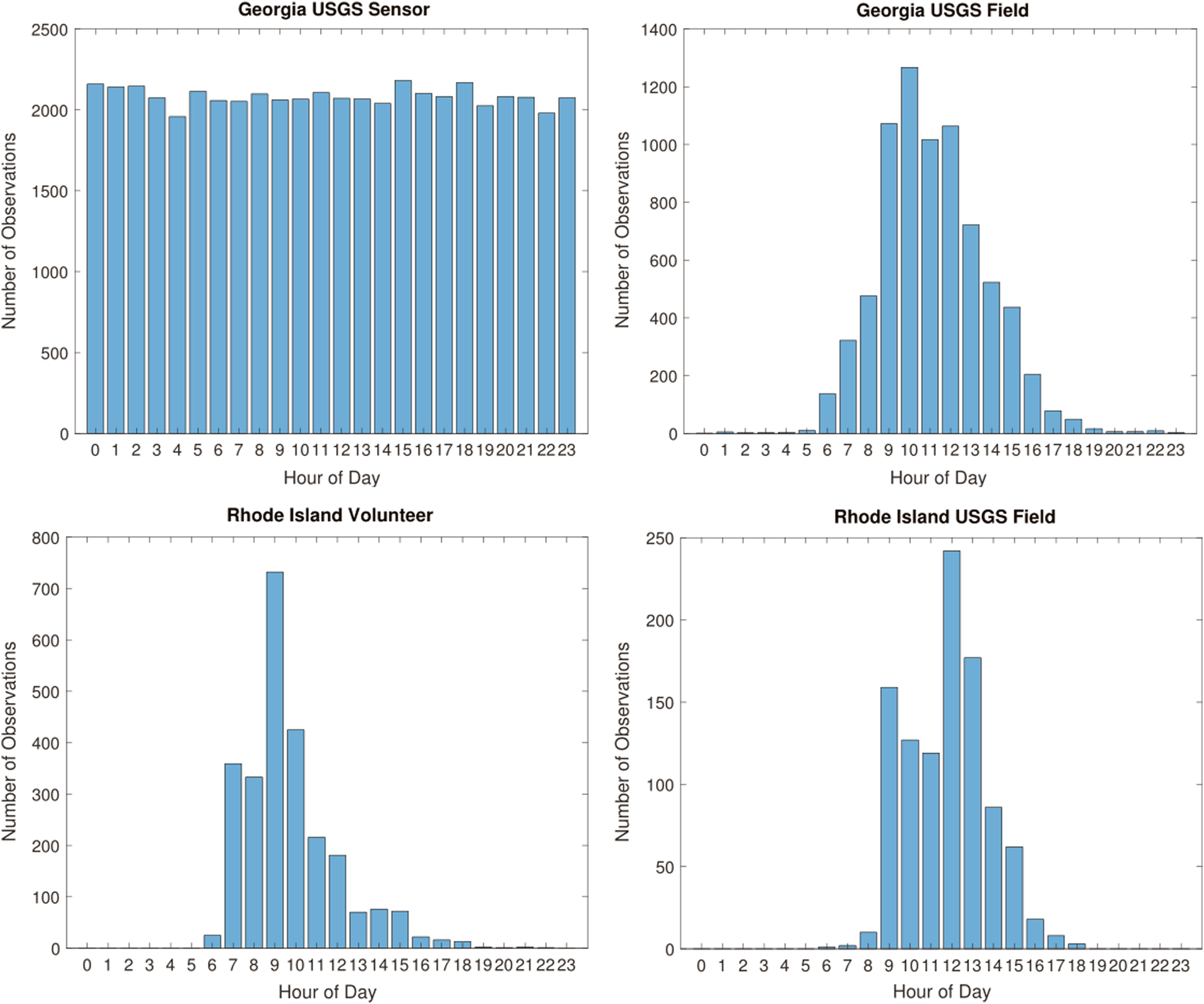
Histograms showing the number of observations collected at each hour of the day for each of the four data samples for which these data were available. Binning was performed by rounding times of collection down to the nearest hour (i.e., 4:01 AM and 4:59 AM would both be tallied in the 4:00 AM bin). Note that time-of-day data were available for only 2,546 of the 5,607 observations in the URIWW data sample. URIWW, University of Rhode Island Watershed Watch.

The distribution of the random sample of sensor-collected data is, as expected, much more evenly distributed across the time-of-day spectrum. To determine whether or not the nighttime sensor observations substantially affected the central tendency of the data, a new random sample of 50,000 observations was generated from the subset of observations collected between 5 AM and 7 PM (the time interval that contains almost all of the human-collected data), and the analysis described in the Data Analysis section was repeated. DO levels in the daytime sensor data sample were found to be an average of 0.1258 mg/L higher than DO levels in the original data sample. This difference is not insignificant, but nevertheless explains only a small portion of the observed discrepancies between the data collected by USGS sensors and the data collected by volunteers.

Site characteristics

The concentration of DO in a river or stream is affected by many site-specific characteristics, including ambient temperature and pressure, aeration, ion activity, aerobic decomposition, ammonia nitrification, and other aquatic chemical and biological reactions (Rounds et al., 2013). This analysis relies on large data sample sizes to limit the effect of random variation in site characteristics on observed DO levels and facilitate credible comparison of observations across data samples. We acknowledge, however, that large sample sizes cannot eliminate systemic bias for one or more of the data samples. Perhaps volunteers more often sample sites characterized by lower DO levels, such as polluted waters near highly populated areas. Perhaps USGS scientists more often sample sites with unusual characteristics. More work should be done to investigate the risk of systemic bias in site selection. As a first step, the location of each observation contained in the data samples was geographically mapped (Figs. 4 and 5). It is clear that volunteer and USGS field sampling sites alike cover a broad geographic range in Georgia and Rhode Island. The regions that account for the bulk of volunteer-collected observations are also heavily sampled by the USGS, and the volunteer-collected observations that report particularly low DO were taken at many different sites. Indeed, if anything, site selection would be expected to push average DO levels recorded in the USGS field data sample downward because more of the USGS field sampling sites are located in Georgia's low-DO Coastal Plain.

FIG. 4.

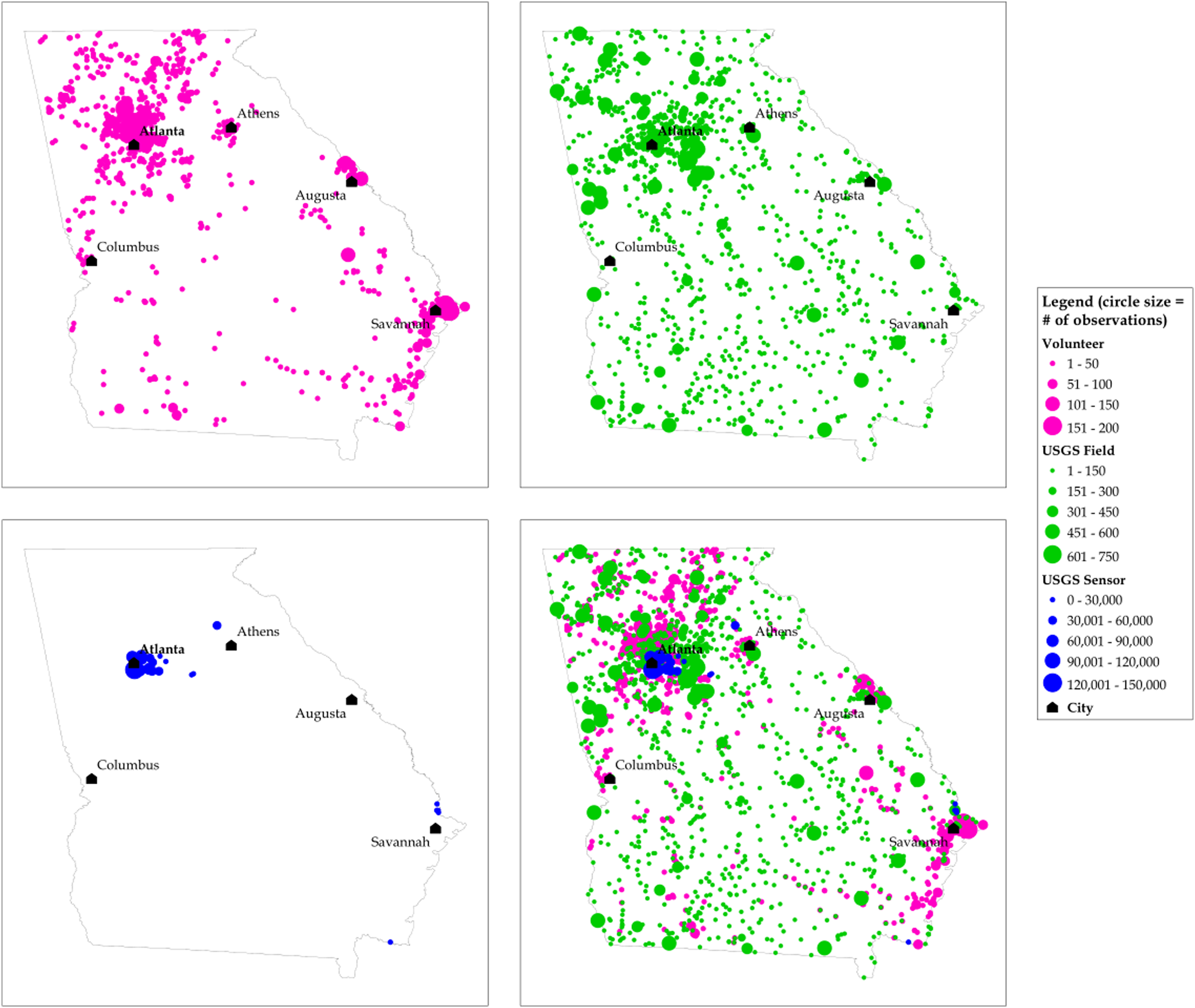
Maps showing sampling sites for Georgia data. Each circle represents a location at which at least one observation (containing both DO and water temperature measurements) was made between January 1995 and October 2016. The size of the circles represents the number of observations collected at each location (note different scales used for circle size for each of the three data samples). The locations of major cities are also marked. Clustering of volunteer monitoring sites near population centers is likely reflective of the fact that participants in the Georgia AAS program are allowed to freely select where and how often to sample. Animated versions of these maps are available online at https://goo.gl/z96V9Q. AAS, Adopt-A-Stream.

FIG. 5.

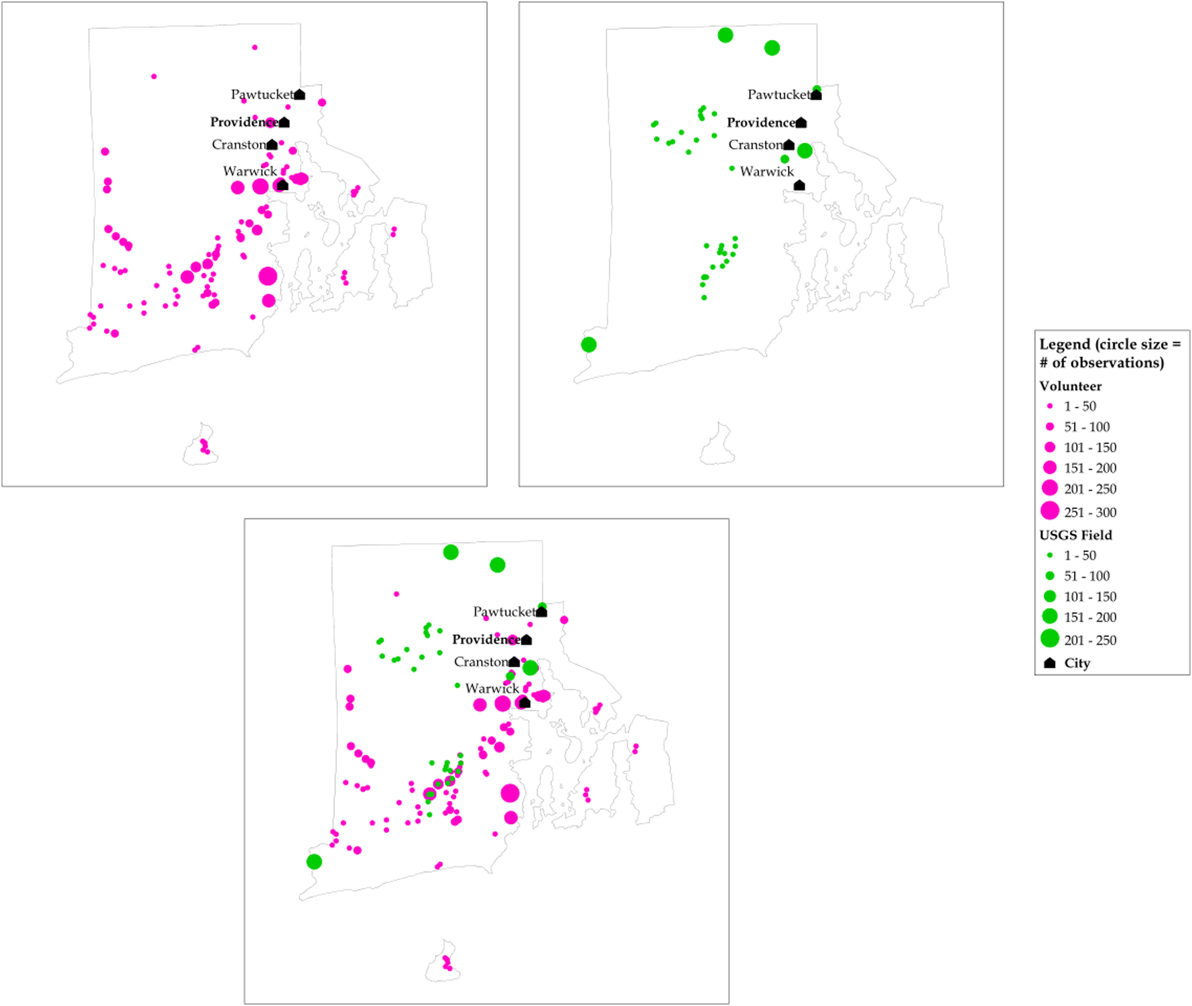
Maps showing sampling sites for Rhode Island data. Each circle represents a location at which at least one observation (containing both DO and water temperature measurements) was made between May 1992 and April 2014. The size of the circles represents the number of observations collected at each location (note different scales used for circle size for each of the three data samples). The locations of major cities are also marked. The relatively even spatial distribution of volunteer monitoring sites is likely reflective of the fact that participants in the URIWW program are told where and how often to sample. Animated versions of these maps are available online at https://goo.gl/n090qE.

Instrumentation, sampling procedure, and personnel training

The USGS uses a variety of optical (luminescence), amperometric, and spectrophotometric sensors to collect both discrete and continuous DO measurements and trains its scientists to follow rigorous calibration, sampling, and reporting protocols in collecting data.^† Instrumentation used by the USGS can be quite expensive, with individual sensors costing thousands of dollars or more. Such detailed protocols and expensive equipment are clearly infeasible for large-scale volunteer monitoring programs such as Georgia AAS and URIWW. These programs instead rely on simpler instrumentation and QA/QC measures. Georgia AAS and URIWW both recommend that participants measure DO using inexpensive, easily obtainable, iodometric (Winkler) titration kits and provide nontechnical step-by-step manuals to guide DO data collection.^‡ Iodometric test kits are inexpensive and easy to obtain, making them well suited for use in large volunteer monitoring programs. However, the USGS has noted several problems with the iodometric method, namely that (1) the accuracy and reproducibility achievable are dependent on the experience and expertise of the data collector, (2) potential environmental interferences (for example, the presence of nitrite, ferrous and ferric iron, and organic matter) require advanced knowledge of the chemistry of the sample, and (3) field conditions can make preventing exposure of the sample to atmospheric oxygen difficult (Rounds et al., 2013). Indeed, Georgia AAS staff have observed that even when performed by trained personnel, DO measurements made using Winkler titration tend to read lower than measurements made on identical samples using more sophisticated equipment (Harold Harbert, personal communication, June 1, 2017).

The discrepancy between volunteer-collected data and USGS-collected data is larger for the URIWW program. This is notable because URIWW provides stricter oversight of volunteers. URIWW specifies monitoring sites and schedules, while Georgia AAS does not. URIWW also requires volunteers to commit to regular participation, while Georgia AAS allows volunteers to sample as frequently or infrequently as they wish. The fact that there is still such a large discrepancy between USGS-collected data and data collected by URIWW volunteers suggests that modest increases in training and supervision have little or no effect on volunteer ability to accurately perform tasks (such as carrying out iodometric titration) characterized by relatively large opportunities for human error. This is consistent with previous findings (e.g., Kosmala et al., 2016) that volunteer accuracy is correlated with task difficulty. More research should be done to determine the extent to which significantly more rigorous training, more detailed sampling protocols, and/or more sophisticated instrumentation can improve volunteer accuracy in DO monitoring.

Comparison of observed and predicted equilibrium DO

The results show that all three data sources report consistently lower DO than the temperature-dependent equilibrium prediction, with the difference largest for volunteer-collected data. This difference is likely attributable to environmental factors not represented in the Benson–Krause model. In Georgia, for instance, many streams and rivers lie in the state's southeastern Coastal Plain region. The Coastal Plain is characterized by slow-moving water bodies that lie adjacent to wetlands and have high sediment oxygen demand and concentrations of organic matter—conditions that result in low DO (Todd et al., 2007). Indeed, as shown in Fig. 6, most of the streams and rivers listed as impaired by the Georgia Department of Environmental Protection due to DO violations lie in the Coastal Plain. In Rhode Island, conditions are not as conducive to naturally low DO (hence the smaller mean difference between USGS field observations and predicted values in Rhode Island relative to Georgia), but sediment oxygen demand, the presence of dissolved organic matter, and other complicating factors may still cause observed DO values to be lower than predicted.

FIG. 6.

Map indicating locations of low-DO freshwater in Georgia. Red lines are streams and rivers listed as impaired by the Georgia Department of Environmental Protection for DO violations.

Spatial and temporal distribution of observations

The second objective of this article was to assess the potential of citizen science to expand spatial and temporal coverage of water monitoring networks. Figures 4 and 5 show the spatial distribution of volunteer sampling sites. In Georgia, results are mixed. The spatial distribution of volunteer sampling sites is much greater than the spatial distribution of USGS sensor sites, but is still concentrated near urban areas and not as great as the spatial distribution of USGS field sampling sites. The number of observations per site also tends to be smaller for volunteer sampling sites than for USGS field sampling sites and much smaller than for USGS sensor sites. In Rhode Island, there is less overlap between volunteer and USGS field sampling sites, and the number of observations per site is about the same. It is also notable that Georgia AAS and URIWW have grown over time. The histograms contained in Fig. 7 show a steady increase in the number of observations collected by volunteers in both programs, and the map animations^§ show that this trend has been driven not only by increases in the number of observations per site but also by increases in the number of sites being sampled.

FIG. 7.

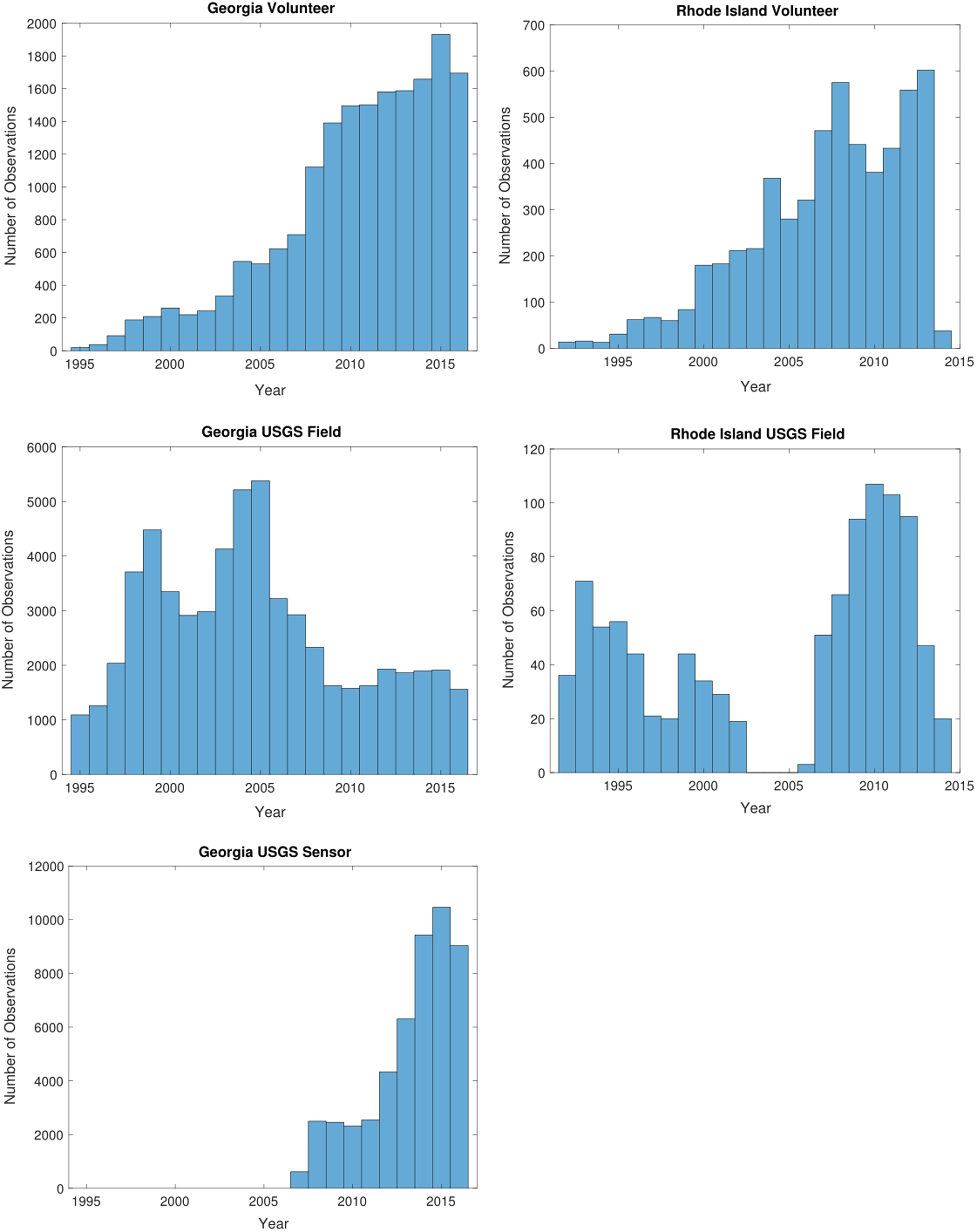
Histograms showing the number of observations collected each year for each of the five data samples. The apparent sudden drop in the number of observations collected by URIWW participants reflects the time range of the data sample.

These results suggest that when volunteers are allowed to freely select where and how often to sample (as is the case for Georgia AAS), monitoring sites will be clustered close to population centers and will tend to be sampled less frequently over time, and a relatively large number of people will participate. When volunteers are told where and how often to sample (as is the case for URIWW), the spatial and temporal distribution of observations will be more even, but participation will be more limited. A hybrid of these approaches, such as a volunteer monitoring program in which participants are encouraged, but not required, to collect data in high-priority or undersampled areas, could provide a valuable complement to USGS field monitoring networks and to support scientific and management efforts for which periodic observations are sufficient. This is especially important given that the number of observations collected by USGS scientists in the two states has remained stagnant over the past two decades. Further work should be done to assess the potential of citizen science to support applications for which continuous data are required.

Footnotes

Author Disclosure Statement

No competing financial interests exist.

*

In September 2015, the U.S. government released an online toolkit (available at: https://crowdsourcing-toolkit.sites.usa.gov) to help federal employees use crowdsourcing and citizen science in their work, and Dr. John P. Holdren, Assistant to the President for Science and Technology and Director of the White House Office of Science and Technology Policy, issued a memo (available at: ) directing the heads of Executive Departments and Agencies to use citizen science and crowdsourcing in addressing societal needs and accelerating science, technology, and innovation.

†

Protocols for field DO measurements are documented by Rounds et al., 2013; protocols for data collection from continuous water-quality monitors are documented by Wagner et al., .

‡

See the Georgia AAS “Physical/Chemical Monitoring” manual (available at: http://adoptastream.georgia.gov/manuals) and the URIWW “Specific Monitoring Techniques” manual (available at: ).

§

Animations of the sampling site maps in Fig. 4 and 5 are available online at: https://goo.gl/z96V9Q and .

References

Benson

B.B.

, and Krause

Jr . (1976). Empirical laws for dilute aqueous solutions of nonpolar gases. J. Chem. Phys., 64, 689.

Benson

B.B.

, and Krause

Jr . (1980). The concentration and isotopic fractionation of gases dissolved in freshwater in equlibrium with the atmosphere. 1. Oxygen. Limnol. Oceanogr., 25, 4.

Benson

B.B.

, and Krause

Jr . (1984). The concentration and isotopic fractionation of oxygen dissolved in freshwater and seawater in equilibrium with the atmosphere. Limnol. Oceanogr., 29, 3.

Canfield

D.E.

Jr. , Brown

C.D.

, Bachmann

R.W.

, and Hoyer

M.V.

(2002). Volunteer lake monitoring: Testing the reliability of data collected by the Florida LAKEWATCH Program. Lake Reserv. Manage., 18, 1.

Connecticut Department of Energy and Environmental Protection (Connecticut DEEP). (2013). A Tiered Approach for Citizen-Based Monitoring of Wadeable Streams and Rivers. Hartford, CT: Connecticut Department of Energy and Environmental Protection. Available at: www.ct.gov/deep/lib/deep/water/volunteer_monitoring/tierapp.pdf (accessed September 12, 2017).

Deutsch

W.G.

, and Ruiz-Córdova

S.S.

(2015). Trends, challenges, and responses of a 20-year, volunteer water monitoring program in Alabama. Ecol. Soc., 20, 3.

Escriva-Bou

, McCann

, Hanak

, Lund

, and Gray

(2016). Accounting for California's Water. Public Policy Institute of California. Available at: www.ppic.org/content/pubs/report/R_716EHR.pdf (accessed September 12, 2017).

Farnham

D.J.

, Gibson

R.A.

, Hsueh

D.Y.

, McGillis

W.R.

, Culligan

P.J.

, Zain

, and Buchanan

(2017). Citizen science-based water quality monitoring: Constructing a large database to characterize the impacts of combined sewer overflow in New York City. Sci. Total Environ., 580, 168–177.

Follet

, and Strezov

(2015). An analysis of citizen science based research: Usage and publication patterns. PLoS One. 10, 11.

10.

Fore

L.S.

, Paulsen

, and O'Laughlin

(2001). Assessing the performance of volunteers in monitoring streams. Freshwater Biol. 46, 1.

11.

Fuccillo

K.K.

, Crimmins

T.M.

, de Rivera

C.E.

, and Elder

T.S.

(2015). Assessing accuracy in citizen science-based plant phenology monitoring. Int. J. Biometeorol., 59, 7.

12.

Hirsch

R.M.

, and Fisher

G.T.

(2014). Past, present, and future of water data delivery from the U.S. Geological Survey. J. Contemp. Water. Res. Educ., 153, 1.

13.

Hoyer

M.V.

, Wellendorf

, Frydenborg

, Bartlett

, and Canfield

D.E.

Jr . (2012). A comparison between professionally (Florida Department of Environmental Protection) and volunteer (Florida LAKEWATCH) collected trophic state chemistry data in Florida. Lake Reserv. Manage., 28, 4.

14.

Illinois Environmental Protection Agency (Illinois EPA). (2015). Tiered Approach. Available at: www.epa.illinois.gov/topics/water-quality/monitoring/vlmp/tiered-approach/index (accessed September 12, 2017).

15.

Kelly

, Champ

, McDonnell

, Kelly-Quin

, Harrison

, Arbuthnott

, Giller

, Joy

, McCarthy

, Cullen

, Harrod

, Jordan

, Griffiths

, and Rosell

(2007). Investigation of the Relationship between Fish Stocks, Ecological Quality Ratings (Q-values), Environmental Factors and Degree of Eutrophication. Environmental Protection Agency, Ireland. Available at: www.epa.ie/wfdstatus/rivers/RW_Fish_River_Methods_ERTDI_Report_73.pdf (accessed September 12, 2017).

16.

Kosmala

, Wiggins

, Swanson

, and Simmons

(2016). Assessing data quality in citizen science. Front. Ecol. Environ., 14, 10.

17.

Lapowsky

(2017). No One Has the Data to Prevent the Next Flint. Wired. Available at: www.wired.com/story/data-lead-poisoning-flint/ (accessed September 12, 2017).

18.

Loperfido

J.V.

, Beyer

, Just

C.J.

, and Schnoor

J.L.

(2010). Uses and biases of volunteer water quality data. Environ. Sci. Technol., 44, 19.

19.

National Water Quality Monitoring Council (NWQMC). (n.d.). Volunteer Monitoring. Advisory Committee on Water Information. Available at: https://acwi.gov/monitoring/vm/index.html (accessed September 12, 2017).

20.

New Jersey Department of Environmental Protection (NJ DEP). (n.d.). Volunteer Monitoring in New Jersey: Connecting Citizens to Science for Better Resource Management. Available at: http://www.nj.gov/dep/wms/volunteer%20poster%20final.pdf (accessed September 12, 2017).

21.

Penn

M.R.

, Pauer

J.J.

, and Mihelcic

J.R.

(2009). Biochemical oxygen demand. In Sabljic

, Ed., Environmental and Ecological Chemistry, Volume II. Oxford: Eolss Publishers Co. Ltd., pp. 278–297.

22.

Rise of the citizen scientist. (2015). Editorial. Nature, 524, 7565.

23.

Rounds

S.A.

, Wilde

F.D.

, and Ritz

G.F.

(2013). Dissolved Oxygen (ver 3.0): U.S. Geological Survey Techniques of Water-Resources Investigations, book 9, chap. A6, sec. 6.2. Reston, VA: United States Geological Survey. Available at: https://water.usgs.gov/owq/FieldManual/Chapter6/6.2/_ver3.pdf (accessed September 12, 2017).

24.

Shelton

A.M.

(2013). The Accuracy of Water Quality Monitoring: A Comparison Between Citizen Scientists and Professionals. Halifax, Nova Scotia: Saint Mary's University. Available at: http://library2.smu.ca/handle/01/25027/-.WMK6VBIrJR0 (accessed September 12, 2017).

25.

Storey

R.G.

, Wright-Stow

, Kin

, Davies-Colley

R.J.

, and Stott

(2016). Volunteer stream monitoring: Do the data quality and monitoring experience support increased community involvement in freshwater decision making?. Ecol. Soc., 21, 4.

26.

Todd

M.J.

, Vellidis

, Lowrance

R.R.

, and Pringle

C.M.

(2007). Low Dissolved Oxygen Levels in Georgia Floodplain Swamps: Effect of Flowpath and Sediment Oxygen Demand. Minneapolis, MN: American Society of Agricultural and Biological Engineers Annual Meeting, pp. 17–20.

27.

United States Environmental Protection Agency (U.S. EPA). (2003). Applying for and Administering CWA Section 319 Grants: A Guide for State Nonpoint Source Agencies. Available at: www.epa.gov/sites/production/files/2015-09/documents/319applying-guide-revised.pdf (accessed September 12, 2017).

28.

United States Geological Survey (USGS). (2011). Office of Water Quality Technical Memorandum 2011.03. Available at https://water.usgs.gov/admin/memo/QW/qw11.03.pdf (accessed September 12, 2017).

29.

USGS. (2017). Water properties: Dissolved oxygen. Available at: https://water.usgs.gov/edu/dissolvedoxygen.html (accessed September 12, 2017).

30.

Wagner

R.J.

, Boulger

R.W.

Jr. , Oblinger

C.J.

, and Smith

B.A.

(2006). Guidelines and Standard Procedures for Continuous Water-Quality Monitors—Station Operation, Record Computation, and Data Reporting. Reston, VA: United States Geological Survey. Available at: https://pubs.usgs.gov/tm/2006/tm1D3/pdf/TM1D3.pdf (accessed September 12, 2017).