Influence of Nonwetting Phase Saturation on Dispersivity in Laboratory-Scale Sandy Porous Media

Abstract

Quantification of dispersive mixing is critically important for characterizing and predicting solute transport in porous media. Dispersion is often estimated by fitting to data collected from a nonreactive, conservative tracer test. While this approach may provide quality estimates, the estimate is specific to the site, soil, or experimental conditions in which the test occurred. Currently, there are a limited number of a priori models for estimating dispersivity in fully saturated or air–water systems and no predictive models to account for the presence of nonaqueous phase liquids (NAPL). The overall goal of this study was to critically assess both established and new models to predict dispersivity based on properties of the porous medium and fluid saturation. To accomplish this, we assembled and reviewed existing laboratory scale dispersivity datasets in sandy porous media. Only 2 of the 10 existing model formulations offer predictive capability (as indicated through Nash–Sutcliffe efficiency [NSE]). This article describes the development of new, empirical models that enhance the ability to predict dispersivity in laboratory-scale water-saturated (NSE increases from 0.40 to 0.83) and air–water (NSE increases from −1.1 to 0.75) systems of sandy porous media. Knowledge of dispersivity under water-saturated conditions further improves prediction of dispersivity in the presence of a nonwetting phase (NSE = 0.90). The resulting models have utility for systems with transient water saturation, such as those experienced during infiltration and irrigation events, NAPL source depletion, and delivery of foams and emulsions used in site remediation.

Introduction

The magnitude of dispersive mixing is critically important when describing or engineering the physical, chemical, and biological processes affecting solutes in the subsurface (e.g., Vanderborght and Vereecken, 2007; Jimenez-Martinez et al., 2015). In fully saturated systems, traditionally hydrodynamic dispersion (D_h) is assumed to have a linear dependence on pore water velocity (v_x), where dispersivity (α) acts as the constant of proportionality (e.g., Saffman, 1959; Scheidegger, 1960; Bear, 1972). Over the past few decades, the mixing literature has focused on elucidating the effects of flow on mixing. For example, the functional form of D_h ∝ v_i ^β (e.g., Bear, 1972; Yule and Gardner, 1978; De Smedt and Wierenga, 1979; Freeze and Cherry, 1979; Fattah and Hoopes, 1985; Hassanizadeh, 1996; Maraqa et al., 1997; Padilla et al., 1999) has been widely investigated and debated, whereas others have correlated D_h to dimensionless flow metrics such as Peclet number and Schmidt number (e.g., Delgado, 2007). Such correlations provide information about the influence of flow behavior on overall dispersive mixing (D_h) rather than revealing information about the dispersivity (α) value itself. Others have focused on nonreactive, conservative tracer behavior marked by early breakthrough and extended tailing and developed approaches such as: (i) a mobile–immobile water content model—with larger immobile water fraction at lower water contents (e.g., De Smedt and Wierenga, 1979; Bond and Wierenga, 1990; Maraqa et al., 1997; Padilla et al., 1999); or (ii) continuous time random walk descriptions (e.g., Cortis and Berkowitz, 2004).

Studies focused on linking dispersion observed in fully saturated media to properties of the porous medium (e.g., Rumer, 1962; Klotz, 1975; Klotz et al., 1980; Menzie and Dutta, 1988) frequently employ grain size, with some postulating that α is directly proportional to the median grain size (d₅₀) (e.g., Perkins and Johnson, 1963; Fried and Combarnous, 1971) as well as soil hydraulic properties (Perfect et al., 2002) (see Table 1 for models). In air–water systems, dispersivity has been related to properties of the porous medium and the condition of fluid saturation (Menzie and Dutta, 1988). In a series of articles Klotz and coworkers identified porosity, effective grain size, deviation of grain shape from a sphere, roughness, and angularity of grains, and the uniformity index as the porous media factors that influence dispersivity (Klotz, 1975; Klotz et al., 1980). Additionally, water content has been frequently correlated to dispersivity to account for the influence of fluid saturation on mixing conditions (e.g., Scheidegger, 1961; Nielsen and Biggar, 1962; Krupp and Elrick, 1968; Conca and Wright, 1992; Conca and Wright,1992; Jardine et al., 1993; Padilla et al., 1999; Toride et al., 2003; Torkzaban et al., 2006; Bunsri et al., 2008; Szenknect et al., 2008).

Table 1.

Existing Literature Dispersivity Models

Longitudinal dispersivity, α_x
	NSE^†/NSE^‡	Source	Notes
Fully saturated systems
\documentclass{aastex}\usepackage{amsbsy}\usepackage{amsfonts}\usepackage{amssymb}\usepackage{bm}\usepackage{mathrsfs}\usepackage{pifont}\usepackage{stmaryrd}\usepackage{textcomp}\usepackage{portland, xspace}\usepackage{amsmath, amsxtra}\usepackage{upgreek}\pagestyle{empty}\DeclareMathSizes{10}{9}{7}{6}\begin{document} $${{ \alpha }} = 1.75 \cdot {{{d}}_{50}}$$ \end{document}	−0.22/−0.59	Perkins and Johnston (1963)
\documentclass{aastex}\usepackage{amsbsy}\usepackage{amsfonts}\usepackage{amssymb}\usepackage{bm}\usepackage{mathrsfs}\usepackage{pifont}\usepackage{stmaryrd}\usepackage{textcomp}\usepackage{portland, xspace}\usepackage{amsmath, amsxtra}\usepackage{upgreek}\pagestyle{empty}\DeclareMathSizes{10}{9}{7}{6}\begin{document} $${{ \alpha }} = 1.7{{{L}}^{1.5}}$$ \end{document}	0.53/0.40	Neuman (1990)	L is in meters; restricted to L ≤ 100 m
\documentclass{aastex}\usepackage{amsbsy}\usepackage{amsfonts}\usepackage{amssymb}\usepackage{bm}\usepackage{mathrsfs}\usepackage{pifont}\usepackage{stmaryrd}\usepackage{textcomp}\usepackage{portland, xspace}\usepackage{amsmath, amsxtra}\usepackage{upgreek}\pagestyle{empty}\DeclareMathSizes{10}{9}{7}{6}\begin{document} $$ { { \alpha } } = 0.5 \cdot { { { d } } _ { 50 } } \cdot { { { v } } ^ { 1 - { { n } } } } \cdot \displaystyle { { \left( { \frac { { { { d } } _ { 50 } } \cdot { { v } } } { { { { D } } _ { { a } } } } } \right) } ^ { 1 / 5 } } $$ \end{document} for \documentclass{aastex}\usepackage{amsbsy}\usepackage{amsfonts}\usepackage{amssymb}\usepackage{bm}\usepackage{mathrsfs}\usepackage{pifont}\usepackage{stmaryrd}\usepackage{textcomp}\usepackage{portland, xspace}\usepackage{amsmath, amsxtra}\usepackage{upgreek}\pagestyle{empty}\DeclareMathSizes{10}{9}{7}{6}\begin{document} $$5 < {{P}}{{{e}}_{{m}}} < 300$$ \end{document}	−0.20/−0.67	Delgado (2007)	n = velocity exponent; \documentclass{aastex}\usepackage{amsbsy}\usepackage{amsfonts}\usepackage{amssymb}\usepackage{bm}\usepackage{mathrsfs}\usepackage{pifont}\usepackage{stmaryrd}\usepackage{textcomp}\usepackage{portland, xspace}\usepackage{amsmath, amsxtra}\usepackage{upgreek}\pagestyle{empty}\DeclareMathSizes{10}{9}{7}{6}\begin{document} $${Pe_{m}} = \frac {d_{50}{v}} {D_{{a}}}$$ \end{document} as defined by Delgado. Presented equation has been rearranged and solved for α
\documentclass{aastex}\usepackage{amsbsy}\usepackage{amsfonts}\usepackage{amssymb}\usepackage{bm}\usepackage{mathrsfs}\usepackage{pifont}\usepackage{stmaryrd}\usepackage{textcomp}\usepackage{portland, xspace}\usepackage{amsmath, amsxtra}\usepackage{upgreek}\pagestyle{empty}\DeclareMathSizes{10}{9}{7}{6}\begin{document} $${\alpha} = 6.0 \left({\frac {\alpha^{}} {n^{}}}\right) + 0.015$$ \end{document}	−5.2/−0.41	Sato et al. (2003)	\documentclass{aastex}\usepackage{amsbsy}\usepackage{amsfonts}\usepackage{amssymb}\usepackage{bm}\usepackage{mathrsfs}\usepackage{pifont}\usepackage{stmaryrd}\usepackage{textcomp}\usepackage{portland, xspace}\usepackage{amsmath, amsxtra}\usepackage{upgreek}\pagestyle{empty}\DeclareMathSizes{10}{9}{7}{6}\begin{document} $${{{ \alpha }}^<sup></sup>}$$ \end{document} and \documentclass{aastex}\usepackage{amsbsy}\usepackage{amsfonts}\usepackage{amssymb}\usepackage{bm}\usepackage{mathrsfs}\usepackage{pifont}\usepackage{stmaryrd}\usepackage{textcomp}\usepackage{portland, xspace}\usepackage{amsmath, amsxtra}\usepackage{upgreek}\pagestyle{empty}\DeclareMathSizes{10}{9}{7}{6}\begin{document} $${{{n}}^<sup></sup>}$$ \end{document} are van Genuchten soil–moisture parameters
\documentclass{aastex}\usepackage{amsbsy}\usepackage{amsfonts}\usepackage{amssymb}\usepackage{bm}\usepackage{mathrsfs}\usepackage{pifont}\usepackage{stmaryrd}\usepackage{textcomp}\usepackage{portland, xspace}\usepackage{amsmath, amsxtra}\usepackage{upgreek}\pagestyle{empty}\DeclareMathSizes{10}{9}{7}{6}\begin{document} $${{ \alpha }} = 2.30{{{ \psi }}_{{a}}} + 12.7{{b}} - 29.1$$ \end{document}	−709/−642	Perfect et al. (2002)	\documentclass{aastex}\usepackage{amsbsy}\usepackage{amsfonts}\usepackage{amssymb}\usepackage{bm}\usepackage{mathrsfs}\usepackage{pifont}\usepackage{stmaryrd}\usepackage{textcomp}\usepackage{portland, xspace}\usepackage{amsmath, amsxtra}\usepackage{upgreek}\pagestyle{empty}\DeclareMathSizes{10}{9}{7}{6}\begin{document} $${{ \psi }}$$ \end{document} _a = air-entry value [ML⁻¹T²]; b = Campbell exponent [—]Reported model r² = 0.47
Air–water systems
\documentclass{aastex}\usepackage{amsbsy}\usepackage{amsfonts}\usepackage{amssymb}\usepackage{bm}\usepackage{mathrsfs}\usepackage{pifont}\usepackage{stmaryrd}\usepackage{textcomp}\usepackage{portland, xspace}\usepackage{amsmath, amsxtra}\usepackage{upgreek}\pagestyle{empty}\DeclareMathSizes{10}{9}{7}{6}\begin{document} $${{ \alpha }} = - 0.197 \cdot {{{ \theta }}_{{w}}} + 0.087$$ \end{document}	−1.68/−3.04	Maciejewski (1994)	a = 0.197 cmb = 0.087 cm for sandy soil
\documentclass{aastex}\usepackage{amsbsy}\usepackage{amsfonts}\usepackage{amssymb}\usepackage{bm}\usepackage{mathrsfs}\usepackage{pifont}\usepackage{stmaryrd}\usepackage{textcomp}\usepackage{portland, xspace}\usepackage{amsmath, amsxtra}\usepackage{upgreek}\pagestyle{empty}\DeclareMathSizes{10}{9}{7}{6}\begin{document} $${{ \alpha }} = 0.00625 \cdot {{{d}}_{50}} \cdot {{n}} \cdot {{{S}}_{{w}}}^{ - 6 / 5}$$ \end{document}	−2.38/−4.5	Haga et al. (1999)	Rearranged from original correlation of \documentclass{aastex}\usepackage{amsbsy}\usepackage{amsfonts}\usepackage{amssymb}\usepackage{bm}\usepackage{mathrsfs}\usepackage{pifont}\usepackage{stmaryrd}\usepackage{textcomp}\usepackage{portland, xspace}\usepackage{amsmath, amsxtra}\usepackage{upgreek}\pagestyle{empty}\DeclareMathSizes{10}{9}{7}{6}\begin{document} $$Pe = 0.8 \cdot S{w^{ - 1.2}}$$ \end{document} from two single-phase flow experiments
\documentclass{aastex}\usepackage{amsbsy}\usepackage{amsfonts}\usepackage{amssymb}\usepackage{bm}\usepackage{mathrsfs}\usepackage{pifont}\usepackage{stmaryrd}\usepackage{textcomp}\usepackage{portland, xspace}\usepackage{amsmath, amsxtra}\usepackage{upgreek}\pagestyle{empty}\DeclareMathSizes{10}{9}{7}{6}\begin{document} $$ { { \alpha } } = \displaystyle \frac { { { { a } } \cdot l } } { 2 } \cdot { { { \theta } } _ { { w } } } ^ { { b } } $$ \end{document}	−317/−540 (l = 23.26)−80.3/−200 (l = L)−2.31/−4.46 (l = d₅₀)	Nützmann et al. (2002)	a = 0.00431133; b = −2.25046; l = characteristic length (23.26 reported)
\documentclass{aastex}\usepackage{amsbsy}\usepackage{amsfonts}\usepackage{amssymb}\usepackage{bm}\usepackage{mathrsfs}\usepackage{pifont}\usepackage{stmaryrd}\usepackage{textcomp}\usepackage{portland, xspace}\usepackage{amsmath, amsxtra}\usepackage{upgreek}\pagestyle{empty}\DeclareMathSizes{10}{9}{7}{6}\begin{document} $$ { { \alpha } } = \displaystyle { \frac { { { { d } } _ { 50 } } } { { { Pe } } } } = { \frac { { { { d } } _ { 50 } } } { { { a } } \cdot { { { S } } _ { { r } } } ^ { { b } } } } $$ \end{document}	−2.66/−2.66 (b = computed)−1.04/−1.08 (b = 2)	Sato et al. (2003)	\documentclass{aastex}\usepackage{amsbsy}\usepackage{amsfonts}\usepackage{amssymb}\usepackage{bm}\usepackage{mathrsfs}\usepackage{pifont}\usepackage{stmaryrd}\usepackage{textcomp}\usepackage{portland, xspace}\usepackage{amsmath, amsxtra}\usepackage{upgreek}\pagestyle{empty}\DeclareMathSizes{10}{9}{7}{6}\begin{document} $$ { { a } } = \displaystyle { \frac { { { { d } } _ { 50 } } } { { { \alpha } } { , _ { { { Sw } } = 1 } } } } $$ \end{document} ; \documentclass{aastex}\usepackage{amsbsy}\usepackage{amsfonts}\usepackage{amssymb}\usepackage{bm}\usepackage{mathrsfs}\usepackage{pifont}\usepackage{stmaryrd}\usepackage{textcomp}\usepackage{portland, xspace}\usepackage{amsmath, amsxtra}\usepackage{upgreek}\pagestyle{empty}\DeclareMathSizes{10}{9}{7}{6}\begin{document} $$ { { b } } = \displaystyle { \frac { \ln \big( { \frac { { { Pe } } } { { a } } } \big) } { \ln ( { { { S } } _ { { w } } } ) } } $$ \end{document} ; \documentclass{aastex}\usepackage{amsbsy}\usepackage{amsfonts}\usepackage{amssymb}\usepackage{bm}\usepackage{mathrsfs}\usepackage{pifont}\usepackage{stmaryrd}\usepackage{textcomp}\usepackage{portland, xspace}\usepackage{amsmath, amsxtra}\usepackage{upgreek}\pagestyle{empty}\DeclareMathSizes{10}{9}{7}{6}\begin{document} $${\\\ {{Pe}} = \displaystyle{{{{{d}}_{50}}{{v}}} \over {{D}}}}$$ \end{document} Authors conclude that b = 2 for all porous media.
Based on fully saturated dispersivity
\documentclass{aastex}\usepackage{amsbsy}\usepackage{amsfonts}\usepackage{amssymb}\usepackage{bm}\usepackage{mathrsfs}\usepackage{pifont}\usepackage{stmaryrd}\usepackage{textcomp}\usepackage{portland, xspace}\usepackage{amsmath, amsxtra}\usepackage{upgreek}\pagestyle{empty}\DeclareMathSizes{10}{9}{7}{6}\begin{document} $$\displaystyle { { \frac { { { { \alpha } } _ { { { unsat } } } } } { { { { \alpha } } _ { { { sat } } } } } } \approx 4 } $$ \end{document}	0.04/0.03 (air–water)−0.58/−0.68 (NAPL)−0.03/−0.08 (Both)	Szenknect et al. (2008)
\documentclass{aastex}\usepackage{amsbsy}\usepackage{amsfonts}\usepackage{amssymb}\usepackage{bm}\usepackage{mathrsfs}\usepackage{pifont}\usepackage{stmaryrd}\usepackage{textcomp}\usepackage{portland, xspace}\usepackage{amsmath, amsxtra}\usepackage{upgreek}\pagestyle{empty}\DeclareMathSizes{10}{9}{7}{6}\begin{document} $$\displaystyle { \frac { { { { \alpha } } _ { { { unsat } } } } } { { { { \alpha } } _ { { { sat } } } } } } \approx 1.9 - 2.8$$ \end{document}	−0.64/−1.05 (c = 1.9, air–water)0.78/0.73 (c = 1.9, NAPL)0.30/0.12 (c = 1.9, Both)−0.04/−0.22 (c = 2.8, air–water)0.71/0.73 (c = 2.8, NAPL)0.95/0.43 (c = 2.8, Both)	Maraqa et al. (1997)
NAPL–water systems
No models found
Transverse (α_y) and vertical (α_z) dispersivity
		Source	Notes
\documentclass{aastex}\usepackage{amsbsy}\usepackage{amsfonts}\usepackage{amssymb}\usepackage{bm}\usepackage{mathrsfs}\usepackage{pifont}\usepackage{stmaryrd}\usepackage{textcomp}\usepackage{portland, xspace}\usepackage{amsmath, amsxtra}\usepackage{upgreek}\pagestyle{empty}\DeclareMathSizes{10}{9}{7}{6}\begin{document} $$\displaystyle \frac { { { { { \alpha } } _ { { y } } } } } { \displaystyle { { { { \alpha } } _ { { x } } } } } = 0.3$$ \end{document} ; \documentclass{aastex}\usepackage{amsbsy}\usepackage{amsfonts}\usepackage{amssymb}\usepackage{bm}\usepackage{mathrsfs}\usepackage{pifont}\usepackage{stmaryrd}\usepackage{textcomp}\usepackage{portland, xspace}\usepackage{amsmath, amsxtra}\usepackage{upgreek}\pagestyle{empty}\DeclareMathSizes{10}{9}{7}{6}\begin{document} $$\displaystyle { \frac { { { { \alpha } } _ { { z } } } } { { { { \alpha } } _ { { x } } } } } = 0.05$$ \end{document}		Lovanh et al. (2000)
\documentclass{aastex}\usepackage{amsbsy}\usepackage{amsfonts}\usepackage{amssymb}\usepackage{bm}\usepackage{mathrsfs}\usepackage{pifont}\usepackage{stmaryrd}\usepackage{textcomp}\usepackage{portland, xspace}\usepackage{amsmath, amsxtra}\usepackage{upgreek}\pagestyle{empty}\DeclareMathSizes{10}{9}{7}{6}\begin{document} $$\displaystyle { \frac { { { { \alpha } } _ { { y } } } } { { { { \alpha } } _ { { x } } } } } = 0.01 - 0.25$$ \end{document}		Bear and Verruijt (1987)

NSE using model to predict dispersivity for the compiled dataset. Where models had specified limiting conditions, the dataset was modified to reflect such conditions. For the models that scale the fully saturated dispersivity to give an estimate of partially saturated mixing, the correlations were computed for air–water systems, NAPL–water systems, and both air–water and NAPL–water systems separately.

†

NSE computed for the full dataset without any exclusion criteria.

‡

NSE computed for the reduced dataset (i.e., Pe < 200 and D_eff/D_h < 10%).

NSE, Nash–Sutcliff efficiency; NAPL, nonaqueous phase liquids.

The influence of entrapped and mobile nonaqueous phase liquids (NAPLs) on dispersivity is often neglected despite several reports that transport properties, including α, are altered in the presence of NAPLs (i.e., air or NAPL) (e.g., Pennell et al., 1993, 1994). In NAPL–water systems, longitudinal dispersivity has been observed to increase with decreasing S_w (Pennell et al., 1993, 1994; Rogers and Logan, 2000; Zhang, et al., 2014). While the NAPL saturations in many of these studies remained low (entrapped saturations that generally produce S_w > 0.8), large increases in α have been observed. Entrapped NAPL saturations commonly result in values of α that are twice that quantified for the same medium when completely water saturated (i.e., comparison between tracer test conducted before and after NAPL entrapment). Still, little research has been conducted to understand the relationship between S_w and α in NAPL–water systems.

Zhang et al. (2014) examined diesel fuel and engine oil (0.6 ≤ S_w ≤ 1.0) and found that the magnitude of increase in α depended on the type of nonaqueous phase. These authors conclude that there was no evidence of chemical or physical nonequilibrium conditions in the columns and postulate effects that are related to blockage of pore spaces, enhancing the local velocity variations. Although the reason for the difference between the results using diesel fuel and engine oil is unclear, Zhang et al. (2014) reported that the spatial nonuniformity of saturation increased with increasing NAPL saturation. Spatially variable water content suggests that some regions of the porous medium may contribute to areas of greater mixing than the overall saturation (or average) would otherwise suggest. The results from Zhang et al. (2014) also suggest that fluid type influences dispersion through the pore-scale NAPL architecture. Effective globule size has been linked to medium and fluid properties, although most typically with d₅₀, uniformity index (U_i), volumetric water content (θ_w), and maximum-entrapped NAPL saturation (e.g., Brusseau et al., 2009; Ramsburg et al., 2011).

Although the influence of water saturation on dispersivity is cited for various partially saturated systems, typically, this phenomenon goes unaccounted for in transport modeling. However, this behavior becomes particularly relevant when considering systems with variable and temporal saturation changes. For example, the use of oil-in-water emulsions to deliver and release remediation amendments (e.g., Long and Borden, 2006; Borden, 2007; Berge and Ramsburg, 2009; Long and Ramsburg, 2011) can alter subsurface saturations (both temporally and spatially) in such a manner that drastically changes dispersive mixing conditions. Similar physics also occur during infiltration and source zone remediation; however, there is no uniform approach to describe these changes in mixing for incorporation into existing models.

The overall objective of this study was to evaluate the predictive capabilities of established and new correlations for estimating α by considering existing data obtained from laboratory-scale experiments in sandy porous media. Relationships were explored for fully and partially water saturated media separately, as well as in combination, with the goal of establishing and quantifying a predictive capability for longitudinal dispersion that can be applied in systems undergoing spatial or temporal changes in water content. By focusing on laboratory-scale systems of sandy porous media, this study removes the influences of texture (e.g., Bromly et al., 2007; Koestel et al., 2012) and scale (e.g., Gelhar et al., 1992) to focus on a set of materials and approaches that are commonly employed when attempting to elucidate complex physical, chemical, and biological processes occurring within the subsurface. Additionally, transverse and vertical dispersivity are commonly estimated as a fraction of longitudinal dispersivity making quality estimates of longitudinal mixing even more valuable (e.g., Bear and Verruijt, 1987; Lovanh et al., 2000). It is in this way that the study aims to provide two foundations for future study: (i) better descriptions of dispersion when interpreting data from laboratory experiments; and (ii) correlation of dispersion to key media and fluid saturation properties that may be expanded upon with considering more complex media.

Methods

Establishment of the dataset

The dataset used herein is compiled from studies available in the peer-reviewed literature. The dataset comprises of both fully and partially saturated experiments conducted under steady flow conditions. Partially saturated data encompass air–water and NAPL–water systems. All studies previously quantified hydrodynamic dispersion coefficient (D_h), Peclet number (Pe), or α by fitting the advection–dispersion equation (ADE) to nonreactive, conservative tracer data. To allow for comparison across all datasets, the analysis herein has been restricted to studies where dispersivity was fit assuming a linear dependence with velocity. Within the ADE, D_h is defined as the sum of effective molecular diffusion, the product of molecular diffusivity (D_a) and tortuosity (τ), and mechanical dispersion, α·v_i [(Eq. (1)]. \documentclass{aastex}\usepackage{amsbsy}\usepackage{amsfonts}\usepackage{amssymb}\usepackage{bm}\usepackage{mathrsfs}\usepackage{pifont}\usepackage{stmaryrd}\usepackage{textcomp}\usepackage{portland, xspace}\usepackage{amsmath, amsxtra}\usepackage{upgreek}\pagestyle{empty}\DeclareMathSizes{10}{9}{7}{6}\begin{document} \begin{align*} {{ {D}}_{{h}}} = {{ {D}}_{ {a}}}{ { \tau + \alpha }} \cdot { {v}}{}_{ {i}} \tag{1} \end{align*} \end{document}

To ensure consistency between studies, reported values of D_h or Pe (as defined in the Notation section) were converted to values of α using \documentclass{aastex}\usepackage{amsbsy}\usepackage{amsfonts}\usepackage{amssymb}\usepackage{bm}\usepackage{mathrsfs}\usepackage{pifont}\usepackage{stmaryrd}\usepackage{textcomp}\usepackage{portland, xspace}\usepackage{amsmath, amsxtra}\usepackage{upgreek}\pagestyle{empty}\DeclareMathSizes{10}{9}{7}{6}\begin{document} $$ { { \alpha = } } { \frac { ( { { { D } } _ { { h } } } - { { { D } } _ { { { eff } } } } ) } { { { { v } } _ { { i } } } } } $$ \end{document} . Here, tortuosity (τ) is calculated as a function of water saturation and porosity through the Millington and Quirk (1961) expression as is common (e.g., default expression in Hydrus). Study selection was limited to laboratory-scale (L ≤100 cm) column experiments using mainly sandy porous media (i.e., glass bead experiments were excluded). In addition, the following properties were required through either direct reporting or inclusion of data that enabled calculation: pore water velocity (v_i), water saturation (S_w), mean grain size diameter (d₅₀), porosity (n), uniformity index (U_i), column length (L), hydrodynamic dispersion coefficient (D_h), and dispersivity (α). The resulting dataset comprised a total of 133 experiments, 63 of which were conducted under fully saturated conditions and 70 under partially saturated conditions (Supplementary Tables S1 and S2, summarized in Table 2).

Table 2.

Data Summary

	All Pe	Pe < 300	Pe < 200
All D_eff/D_h
S_w = 1	67	57	31
S_w < 1	69	69	64
NAPL–water	41	41	37
Air–water	28	28	27
Total	136	126	95
D_eff/D_h < 25%
S_w = 1	59	54	27
S_w < 1	68	68	63
NAPL–water	40	40	36
Air–water	28	28	27
Total	127	122	90
D_eff/D_h < 10%
S_w = 1	34	30	18
S_w < 1	64	64	59
NAPL–water	36	36	32
Air–water	28	28	27
Total	98	94	77

When assessing data, it became necessary to screen out some data to ensure the overall quality of the dataset. Experiments in which: (i) high Pe introduced uncertainty into values of D_h or α; and/or (ii) the effective diffusion contributed appreciably to D_h, were excluded from the analysis. Two thresholds were employed for each of these criteria (Pe < 300 and Pe < 200, and D_eff/D_h < 25% and D_eff/D_h < 10%). The development and rationale of the Pe criteria are explained in more detail below. Final polyparameter models were produced by enforcing the strictest set of criteria (i.e., Pe < 200 and D_eff /D_h<10%). The influence of enforcing these criteria on the quantity of studies in the dataset is shown in Table 2. Pe is defined here using column length (L) as the characteristic length. Care was taken when analyzing literature data as to how Pe was defined in each study, as some studies focused on pore scale processes use d₅₀ to represent characteristic length (i.e., Pe,_d50).

Model development and evaluation

Predictor selection

Selection of predictors for use in the polyparameter model development focused on identifying commonly reported properties of saturated and unsaturated porous media. Porosity, median grain diameter, uniformity index, and bed length were selected as dispersivity has been linked to these routinely quantified porous media properties (e.g., Perkins and Johnston, 1963; Fried and Combarnous, 1971; Menzie and Dutta, 1988; Gelhar et al., 1992). Water content was represented within the polyparameter models as water saturation. Distributions of these properties for the dataset, as well as Pe, D_h, α, and v_i are provided in Fig. 1.

FIG. 1.

Distribution of properties in the dataset. Each panel shows (left to right): fully saturated (S_w = 1); partially saturated (S_w<1); air–water systems; NAPL–water systems; and all data. Boxes denote the 25th and 75th percentiles. Median values are shown as the horizontal line within each box. Tenth and 90th percentiles are shown with whiskers, and outliers noted by the filled circles. NAPL, nonaqueous phase liquids.

Polyparameter model fitting

Polyparameter models were fit using MATLAB R2014a (The Mathworks, Natick, MA). Models were linearized to capitalize on the robustness of the MATLAB linear fitting routine (fitlm) to minimize the sum squared errors. Data were equally weighted in all fits. The resulting equation in its most general form (including all possible predictors) is shown in Equation (2). \documentclass{aastex}\usepackage{amsbsy}\usepackage{amsfonts}\usepackage{amssymb}\usepackage{bm}\usepackage{mathrsfs}\usepackage{pifont}\usepackage{stmaryrd}\usepackage{textcomp}\usepackage{portland, xspace}\usepackage{amsmath, amsxtra}\usepackage{upgreek}\pagestyle{empty}\DeclareMathSizes{10}{9}{7}{6}\begin{document} \begin{align*} \log ({\rm{\hat \alpha }}) = {\rm{a}} \cdot \log ({{\rm{d}}_{50}}) + {\rm{b}} \cdot \log ({\rm{n}}) + {\rm{c}} \cdot \log ({{\rm{U}}_{\rm{i}}}) + {\rm{d}} \cdot \log ({{\rm{S}}_{\rm{w}}}) + {\rm{e}} \cdot \log ({\rm{L}}) + {\rm{\chi }} \tag { 2 } \end{align*} \end{document}

Here, \documentclass{aastex}\usepackage{amsbsy}\usepackage{amsfonts}\usepackage{amssymb}\usepackage{bm}\usepackage{mathrsfs}\usepackage{pifont}\usepackage{stmaryrd}\usepackage{textcomp}\usepackage{portland, xspace}\usepackage{amsmath, amsxtra}\usepackage{upgreek}\pagestyle{empty}\DeclareMathSizes{10}{9}{7}{6}\begin{document} $$\hat \alpha$$ \end{document} is the modeled dispersivity, a–e are fitted model parameters. A model coefficient (χ) was also fit as the omission of this coefficient would imply that α can be entirely described by the predictor variables—a result that has limited physical meaning. Polyparameter models of increasing complexity were systematically tested by adding a new predictor until the addition of another predictor was not statistically significant (i.e., p > 0.05). Model residuals were checked for normality (Anderson-Darling test) and homoscedasticity (Breusch–Pagan test), and multicollinearity between predictors was evaluated (variance inflation factor).

Model evaluation

The capability of existing models (Table 1) to predict dispersivities within the dataset was assessed using Nash–Sutcliffe efficiency (NSE). The developed polyparameter models were evaluated on the basis of NSE; sample size corrected Akaike information criterion (AICc); and adjusted R² (adj-R²).

NSE was calculated as shown in Equation (3) (Nash and Sutcliffe, 1970). \documentclass{aastex}\usepackage{amsbsy}\usepackage{amsfonts}\usepackage{amssymb}\usepackage{bm}\usepackage{mathrsfs}\usepackage{pifont}\usepackage{stmaryrd}\usepackage{textcomp}\usepackage{portland, xspace}\usepackage{amsmath, amsxtra}\usepackage{upgreek}\pagestyle{empty}\DeclareMathSizes{10}{9}{7}{6}\begin{document} \begin{align*} { { NSE } } = 1 - { \frac { \sum { { { ( { { { \alpha } } _i } - { { { { \hat \alpha } } } _ { { i } } } ) } ^2 } } } { \sum { { { ( { { { \alpha } } _ { { i } } } - { { \bar \alpha } } ) } ^2 } } } } \tag { 3 } \end{align*} \end{document}

where α is the observed dispersivity, \documentclass{aastex}\usepackage{amsbsy}\usepackage{amsfonts}\usepackage{amssymb}\usepackage{bm}\usepackage{mathrsfs}\usepackage{pifont}\usepackage{stmaryrd}\usepackage{textcomp}\usepackage{portland, xspace}\usepackage{amsmath, amsxtra}\usepackage{upgreek}\pagestyle{empty}\DeclareMathSizes{10}{9}{7}{6}\begin{document} $${{ \hat \alpha }}$$ \end{document} is the modeled dispersivity, and \documentclass{aastex}\usepackage{amsbsy}\usepackage{amsfonts}\usepackage{amssymb}\usepackage{bm}\usepackage{mathrsfs}\usepackage{pifont}\usepackage{stmaryrd}\usepackage{textcomp}\usepackage{portland, xspace}\usepackage{amsmath, amsxtra}\usepackage{upgreek}\pagestyle{empty}\DeclareMathSizes{10}{9}{7}{6}\begin{document} $${{ \bar \alpha }}$$ \end{document} is the averaged observed dispersivity. NSE values range from −∞ to 1, with a perfect model giving an NSE = 1. Models having NSE < 0 suggest that data are better described using the mean than the model in question.

AICc evaluates goodness of fit with penalties for additional fitting parameters [Eq. (4)] (Akaike, 1974) and was used to select the best model within the subset of data. \documentclass{aastex}\usepackage{amsbsy}\usepackage{amsfonts}\usepackage{amssymb}\usepackage{bm}\usepackage{mathrsfs}\usepackage{pifont}\usepackage{stmaryrd}\usepackage{textcomp}\usepackage{portland, xspace}\usepackage{amsmath, amsxtra}\usepackage{upgreek}\pagestyle{empty}\DeclareMathSizes{10}{9}{7}{6}\begin{document} \begin{align*} { { AICc } } = \left[ { { { N } } \cdot \ln \left( { { \frac { { { SSE } } } { { N } } } } \right) + 2 { { k } } } \right] + { \frac { 2 { { k } } ( { { k } } + 1 ) } { { { N } } - { { k } } - 1 } } \tag { 4 } \end{align*} \end{document}

where N is the number of observations, SSE is the sum squared error, and k is the number of model parameters plus one. Note that the number of model parameters is the number of predictors plus one since χ is also fit.

Transport simulations

A series of transport simulations was conducted to assess the systematical error associated with fitting longitudinal dispersivity values to data obtained from column experiments. This assessment supported the establishment of a set of data quality criteria related to Peclet number. The general approach here was to first simulate tracer transport for a known Peclet number and then discretize the output to mimic how experimental data are often collected in column experiments. Next, the same model was used to fit Pe to the discretized data points (i.e., the standard technique for determining dispersivity from miscible displacement experiments). The known (inputted) Pe was then compared against the fitted Pe value to determine a percent error on α.

Simulations of a one pore volume pulse of a nonreactive, conservative tracer were completed using the CFITM equilibrium transport code in STANMOD v.2.07 (Simunek et al., 2005) for a semi-finite system with a third type boundary condition (van Genuchten, 1980b). Simulations were conducted for 50 ≤ Pe ≤ 400. To produce discretized, simulated data, effluent concentrations from the tracer simulations were averaged over a given sampling period. Sampling frequencies of 10 and 18 samples per pore volume were assessed, as these sampling frequencies are commonly employed in column experiments. Fits of the transport equation to the synthetic data were conducted using CFTIM under the same conditions as described above. Where noted below, experimental uncertainty was approximated by adding 2% Gaussian noise to the synthetic data (SI section 3). These results were used to define data quality thresholds based on the experimental Pe and sampling frequency.

Results and Discussion

Established models for predicting dispersivity

There are several existing models that aim to predict α as a function of properties of the porous medium for both fully and partially saturated media (Table 1). However, only one model (Neuman, 1990; NSE = 0.40) has a NSE substantially greater than zero when applied to the dataset (Table 1, Fig. 2). Recall that NSE < 0 indicates that the average of the data is a stronger predictor than the model being evaluated. Existing models that aim to estimate α in air–water systems based on properties of the porous medium fare poorly (NSE < 0, Table 1, Fig. 2). Predictive capability is only found when considering the subset of air–water models that scale values of α that were measured in the same medium under fully saturated conditions. The advantage of these scaling models is that they remove the need for, and error associated with, estimating α based on properties of the porous media—a task that is difficult. The results shown in Table 1 and Fig. 2 highlight a need to develop new models that can offer a priori estimates longitudinal dispersivity in sandy porous media.

FIG. 2.

Predictive power of existing models for (a) fully saturated media; (b) air–water systems; and (c) partially saturated dispersivity models based on fully saturated dispersivity. Notes: The range of axes values is larger in (a). ¹Air–water expression developed in this study: \documentclass{aastex}\usepackage{amsbsy}\usepackage{amsfonts}\usepackage{amssymb}\usepackage{bm}\usepackage{mathrsfs}\usepackage{pifont}\usepackage{stmaryrd}\usepackage{textcomp}\usepackage{portland, xspace}\usepackage{amsmath, amsxtra}\usepackage{upgreek}\pagestyle{empty}\DeclareMathSizes{10}{9}{7}{6}\begin{document} $${{ \alpha }} ( {{cm}} ) = 0.23 \cdot {{{n}}^{2.2}}{{ \theta }}_{{w}}^{ - 1.3}$$ \end{document} . ²Equation (8) applied while excluding Padilla et al. (1999). See Fig. 5 and related discussion of Padilla et al. (1999). Nützmann et al. (2002) provide a model using a characteristic length (l). Three configurations of the Nützmann et al. model were assessed: l = length of column (L); l = median grain size (d₅₀); and l = 23.26 [fitted value given in Nützmann et al. (2002) article for their column experiments with sandy porous media].

Influence of Peclet number on estimation of alpha

Critical to the development of models that can predict α, is the reliability of α estimates obtained through fitting of tracer breakthrough curves. Fitted values of α depend both on the quality and quantity of data, as well as the appropriateness of the transport model being employed. Within the context of the ADE, Pe serves as the critical description of dispersive mixing. Effective measurement of dispersion in systems comprising of a disproportionate amount of advection, however, can be difficult. For example, nonreactive, conservative tracer tests are routinely conducted through collection of 10–12 effluent samples per pore volume. The concentration of tracer in these samples is quantified and subsequently used to fit the ADE by adjusting a parameter that represents dispersive mixing (Pe, D_h, or α). As Pe increases, this fitting approach is increasingly reliant upon just a few data points corresponding to the rise and fall of the breakthrough curve (BTC). Shown in Fig. 3 are synthetic data that illustrate this point. For each Pe the BTC was simulated and then discretized to 10 “observations” per pore volume by calculating the cumulative solute mass in the effluent over a sampling period and dividing by the cumulative phase volume in the effluent over that period. The tracer simulation for Pe = 200 is shown to illustrate the similarity in the data. These “observations” are then used to produce estimates of Pe using CFTIM, which were compared with the known values of Pe used in the original forward simulation. Results using a 10-sample per pore volume discretization suggest that the percent difference between fitted and known Pe scales linearly with Pe (slope = [4.0 ± 0.1] × 10⁻² for Pe >50) is ∼8% at Pe = 200. Use of 18 samples per pore volume increases the accuracy of the fits by roughly a factor of 3 (Table 3) with percent difference versus Pe producing a slope of (1.4 ± 0.1) × 10⁻² (for Pe > 50). These results suggest that tracer experiments conducted at high Pe may produce less reliable estimates of α. Studies having Pe > 200 were therefore excluded, unless the study was determined to use a higher rate of sampling (i.e., greater than 10 samples per pore volume) (Table 3). Only three such studies are present in the dataset: Pennell et al. (1993, 1994) with ∼15 samples per pore volume, and Zhang et al. (2014) with ∼30 samples per pore volume.

FIG. 3.

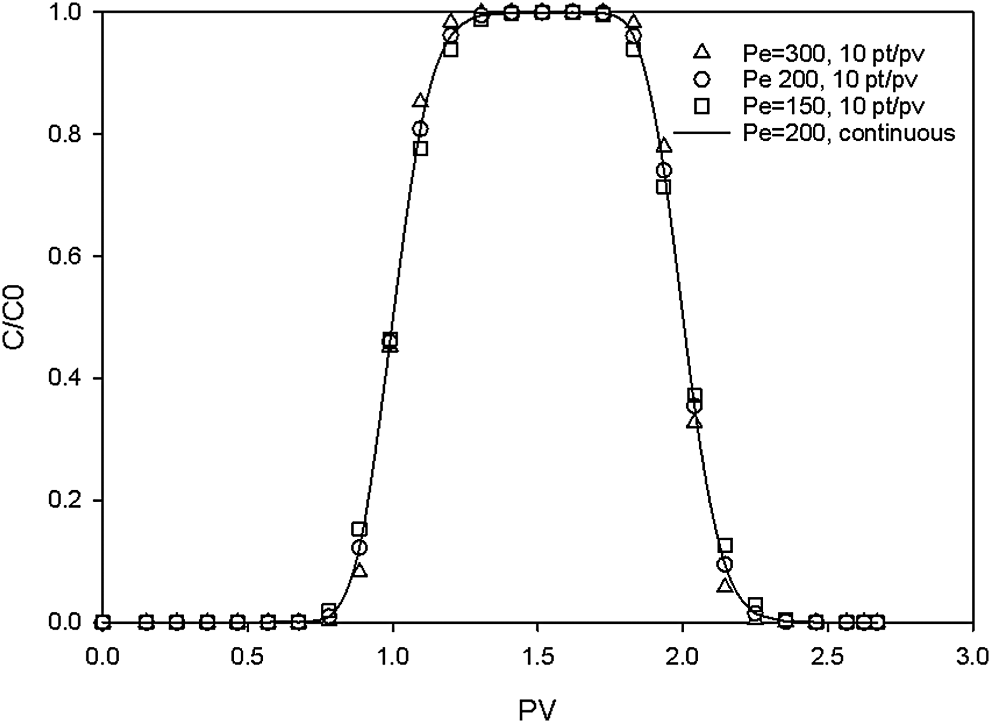
Influence of experimental sampling (i.e., discretization) on simulated tracer transport.

Table 3.

Uncertainty When Fitting Simulated Data After Discretization

	Fitted Pe (95% CI) percent difference with known
Known Pe	Discretized 10 pts/PV	Discretized 18 pts/PV
400	337.5 (334.1, 340.9) 16%	378.5 (377.6, 379.4) 5%
300	263.6 (261.3, 266.0) 12%	287.8 (287.2, 288.4) 4%
250	224.3 (222.4, 226.1) 10%	241.4 (241.0, 241.9) 3%
200	183.3 (181.9, 184.6) 8%	194.5 (194.2, 194.8) 3%
150	140.4 (139.5, 141.3) 6%	146.9 (146.7, 147.1) 2%
125	118.3 (117.5, 119.0) 5%	122.8 (122.7, 123.0) 2%
100	96.0 (95.1, 96.2) 4%	98.6 (98.5, 98.7) 1%
50	48.9 (48.7, 49.1) 3%	49.7 (49.6, 49.7) 1%

New models for predicting dispersivity

Fully saturated media

The single best predictor of the fully saturated data is L ( \documentclass{aastex}\usepackage{amsbsy}\usepackage{amsfonts}\usepackage{amssymb}\usepackage{bm}\usepackage{mathrsfs}\usepackage{pifont}\usepackage{stmaryrd}\usepackage{textcomp}\usepackage{portland, xspace}\usepackage{amsmath, amsxtra}\usepackage{upgreek}\pagestyle{empty}\DeclareMathSizes{10}{9}{7}{6}\begin{document} $${{ \alpha }} ( {{cm}} ) = 2.50 \times {10^{ - 3}} \cdot {{{L}}^{1.49}}$$ \end{document} , with L in cm, NSE = 0.63, AICc = −63.2). When developing single-parameter models, both U_i and n were also found to be statistically significant (p < 0.05); however, the model with U_i resulted in a negative NSE. The model using n had a NSE of 0.54 and AICc of −59.2, which is inferior to that produced with using L as the single predictor. The L^1.5 dependency of this single model is the same as that found by Neuman (1990). The interested reader is referred to Supplementary Fig. S1, which shows the dataset within the context of the Neuman (1990) analysis. Gelhar et al. (1992), in their critical review of field-scale dispersion, note a dependence of dispersion on length scale, but conclude that the Neuman model (i.e., a single value of the exponent on L) oversimplifies the role of heterogeneity at field sites. The agreement in exponent between our study and the work by Neuman likely results from the intentional focus on sandy porous media evaluated at the laboratory scale. This focus removes the important field-scale consideration noted by Gelhar et al. (1992). However, sandy porous media may not be as homogeneous as presumed (e.g., Vogel and Roth, 2003; Zhang et al., 2013; Fitch et al., 2015). This is important as Klotz et al. (1980) suggest that small-scale “geological interfaces” can influence dispersion and adversely affect comparison among laboratory-scale columns. The difference between the model developed in this study and that of Neuman lies in the leading coefficient (Neuman model coefficient is 1.7 × 10⁻³ when adjusted to use cm for both L and α). Recall that the Neuman model was the only existing model for fully saturated systems that had a NSE >0. When applied with the dataset used to develop new models, the Neuman model had a NSE of 0.40 (Table 1, Fig. 2). Reconsideration of the model coefficient improves NSE to 0.63.

Model development also considered two-, three-, and four-predictor models. The best two- and three-predictor models exclude L in favor of U_i and n. The reason for this is unclear, although there is some indication that the longer column experiments contained in the dataset employed finer, more uniform media (Supplementary Fig. S2). The best two-predictor model is \documentclass{aastex}\usepackage{amsbsy}\usepackage{amsfonts}\usepackage{amssymb}\usepackage{bm}\usepackage{mathrsfs}\usepackage{pifont}\usepackage{stmaryrd}\usepackage{textcomp}\usepackage{portland, xspace}\usepackage{amsmath, amsxtra}\usepackage{upgreek}\pagestyle{empty}\DeclareMathSizes{10}{9}{7}{6}\begin{document} $${{ \alpha }} ( {{cm}} ) = 85.2 \cdot {{U}}_{{i}}^{1.14}{{{n}}^{6.86}}$$ \end{document} with a NSE of 0.66. This model represents an addition of one predictor (U_i) to the single-predictor model employing n. Thus, the utility of this two-predictor model is assessed by comparing its AICc value of −61.4 to that is obtained for the model developed with n as a single predictor (AICc of −59.2). Models that individually add d₅₀ (in cm), U_i, and n to the best single-predictor model (L^1.5) produce coefficients that are statistically significant at higher p-values. The best of these two-predictor models is \documentclass{aastex}\usepackage{amsbsy}\usepackage{amsfonts}\usepackage{amssymb}\usepackage{bm}\usepackage{mathrsfs}\usepackage{pifont}\usepackage{stmaryrd}\usepackage{textcomp}\usepackage{portland, xspace}\usepackage{amsmath, amsxtra}\usepackage{upgreek}\pagestyle{empty}\DeclareMathSizes{10}{9}{7}{6}\begin{document} $${{ \alpha }} ( {{cm}} ) = 6.62 \times {10^{ - 3 \cdot }}{{L}}_{}^{1.50}{{{d}}_{50}}^{0.31}$$ \end{document} having a NSE of 0.65 and AICc of −67.7. While the exponent on the d₅₀ has a p-value of 0.16, this combination of NSE and AICc along with the incorporation of L offers a superior description of the dataset.

Three-predictor combinations of L, U_i, n, and d₅₀ lead to similar results regarding the tradeoff between the level of statistical significance of the model parameters, model performance (NSE and AICc), and link to well-established observations that \documentclass{aastex}\usepackage{amsbsy}\usepackage{amsfonts}\usepackage{amssymb}\usepackage{bm}\usepackage{mathrsfs}\usepackage{pifont}\usepackage{stmaryrd}\usepackage{textcomp}\usepackage{portland, xspace}\usepackage{amsmath, amsxtra}\usepackage{upgreek}\pagestyle{empty}\DeclareMathSizes{10}{9}{7}{6}\begin{document} $${{ \alpha }} = {{f}} ( {{L}} )$$ \end{document} . The best three-predictor model in which all coefficients are statistically significant at p < 0.05 is \documentclass{aastex}\usepackage{amsbsy}\usepackage{amsfonts}\usepackage{amssymb}\usepackage{bm}\usepackage{mathrsfs}\usepackage{pifont}\usepackage{stmaryrd}\usepackage{textcomp}\usepackage{portland, xspace}\usepackage{amsmath, amsxtra}\usepackage{upgreek}\pagestyle{empty}\DeclareMathSizes{10}{9}{7}{6}\begin{document} $${{ \alpha }} ( {{cm}} ) = 4965 \cdot {{d}}_{50}^{0.87}{{{n}}^{8.37}}{{U}}_{{i}}^{1.78}$$ \end{document} (NSE of 0.83, AICc of −71.1). Inclusion of L^1.50, however, produces a model of form \documentclass{aastex}\usepackage{amsbsy}\usepackage{amsfonts}\usepackage{amssymb}\usepackage{bm}\usepackage{mathrsfs}\usepackage{pifont}\usepackage{stmaryrd}\usepackage{textcomp}\usepackage{portland, xspace}\usepackage{amsmath, amsxtra}\usepackage{upgreek}\pagestyle{empty}\DeclareMathSizes{10}{9}{7}{6}\begin{document} $${{ \alpha }} ( {{cm}} ) = 0.615 \cdot {{{L}}^{1.50}}{{d}}_{50}^{\,0.53}{{{n}}^{3.72}}$$ \end{document} , where the exponent on n has a p-value of 0.06, and the model has a NSE of 0.86 and AICc of −74.8 (Fig. 4). The addition of a fourth predictor increases AICc, suggesting that the additional fitting parameter cannot be supported. Thus, the recommended model [Eq. (5)] comprises three predictors, and offers a substantial increase in description of the dataset over any currently available model (ΔNSE = 0.43). \documentclass{aastex}\usepackage{amsbsy}\usepackage{amsfonts}\usepackage{amssymb}\usepackage{bm}\usepackage{mathrsfs}\usepackage{pifont}\usepackage{stmaryrd}\usepackage{textcomp}\usepackage{portland, xspace}\usepackage{amsmath, amsxtra}\usepackage{upgreek}\pagestyle{empty}\DeclareMathSizes{10}{9}{7}{6}\begin{document} \begin{align*} {{ \alpha }} ( {{cm}} ) = 0.615 \cdot {{{L}}^{1.50}}{{d}}_{50}^{0.53}{{{n}}^{3.72}} \tag{5} \end{align*} \end{document}

FIG. 4.

Performance of best-fit models for dispersivity reported in cm: fully saturated [left; Eq. (5)]; partially saturated [middle; Eq. (6)]; and all data [right, Eq. (7)].

Partially saturated media

The partially saturated experiments in the dataset comprise both NAPL–water and air–water systems. The single best predictor for the partially saturated data is S_w (AICc = −283.8, adj-R² = 0.55, NSE = 0.53), with d₅₀ and S_w comprising the best two-predictor models (AICc = −292.1, adj-R² = 0.61, NSE = 0.61). The best-fit model includes five predictors as shown in Equation (6) (AICc = −320.4, adj-R² = 0.77, NSE = 0.78, Fig. 4). \documentclass{aastex}\usepackage{amsbsy}\usepackage{amsfonts}\usepackage{amssymb}\usepackage{bm}\usepackage{mathrsfs}\usepackage{pifont}\usepackage{stmaryrd}\usepackage{textcomp}\usepackage{portland, xspace}\usepackage{amsmath, amsxtra}\usepackage{upgreek}\pagestyle{empty}\DeclareMathSizes{10}{9}{7}{6}\begin{document} \begin{align*} {{ \alpha }} ( {{cm}} ) = 161 \cdot {{S}}_{{w}}^{ - 1.31}{{d}}_{50}^{0.35}{{{n}}^{6.5}}{{{L}}^{ - 0.72}}{{U}}_{{i}}^{1.73} \tag{6} \end{align*} \end{document}

When treated individually (Supplementary Fig. S3), the single best predictors for the air–water and NAPL–water are S_w (AICc = −135.5, adj-R² = 0.66, NSE = 0.66) and d₅₀ (AICc = −168.2, adj-R² = 0.49, NSE = 0.49), respectively. Both of these single-predictor models offer strong performance. The selection of S_w as the best single predictor for the air–water system is well aligned with the many studies identifying a dependence of dispersive mixing on S_w (as water content, θ_w) (Conca and Wright, 1992; Haga et al., 1999; Sato et al., 2003).

The air–water model suggests an inverse relationship between S_w and α.

In contrast, S_w is not statistically significant as a single predictor for the NAPL–water subset of data (NAPL–water model suggests an inverse relation between d₅₀ and α). We suspect S_w is not the best single predictor of the NAPL–water subset of studies due to the relatively narrow range of S_w created by the entrapped NAPL saturations that comprise the subset (Fig. 1).

The influence of d₅₀, n, and L in the partially saturated case [Eq. (6)] differs from that established for the fully saturated case [Eq. (5)]. We hypothesized that these predictors are contributing information related to the configuration of nonwetting (or wetting) phase at the pore scale. For the purposes of this study, we assume all nonwetting phase saturations are uniform at the column scale. However, imaging studies demonstrate that nonwetting phase spans multiple pore bodies in ways that require saturation to be defined using averaging volumes that are greater than those used for defining porosity (e.g., Georgiadis et al., 2013). The indirect relationship between α and L in Equation (6) may represent the influence of averaging volume (used to establish the uniform value of S_w) on the reported value of dispersivity. In other words, the distribution of nonwetting phase may have an important role in local mixing–one which is not always well described at the column scale when fitting the ADE to a tracer breakthrough curve. Interestingly, d₅₀, U_i, n, and S_w have all been shown to be useful when characterizing the effective size of NAPL ganglia (e.g., Brusseau et al., 2009; Ramsburg et al., 2011). The fact that the best-fit model for the partially saturated data [Eq. (6)] contains these predictors appears to suggest that the model partially captures the role of the interconnectedness of the nonwetting phase on mixing. This observation aligns with previous findings related to how the saturation and interconnectedness of the saturation influences tortuosity and mixing (e.g., Wildenschild and Jensen, 1999; Rossi et al., 2007). The statistical differences between the coefficients on d₅₀, U_i, and n for the fully and partially saturated models also suggest that these predictors provide information on both the porous medium and the distribution of the water therein.

Combined model

To explore the possibility of obtaining a model capable of describing transitions between fully saturated and partially saturated conditions, we pursued two lines of inquiry–(1) model the full dataset (fully and partially saturated data) using the approach described above, and (2) examine the subset of data for which tracer tests occurred in the same medium under both fully and partially saturated conditions. When data are combined, the resulting best-fit polyparameter model is the five-parameter model shown in Equation (7). \documentclass{aastex}\usepackage{amsbsy}\usepackage{amsfonts}\usepackage{amssymb}\usepackage{bm}\usepackage{mathrsfs}\usepackage{pifont}\usepackage{stmaryrd}\usepackage{textcomp}\usepackage{portland, xspace}\usepackage{amsmath, amsxtra}\usepackage{upgreek}\pagestyle{empty}\DeclareMathSizes{10}{9}{7}{6}\begin{document} \begin{align*} {{ \alpha }} ( {{cm}} ) = 758 \cdot {{d}}_{50}^{0.61}{{S}}_{{w}}^{ - 1.1}{{{n}}^{7.3}}{{{L}}^{ - 0.55}}{{U}}_{{i}}^{2.0} \tag{7} \end{align*} \end{document}

The inverse dependence of this model is consistent with other studies examining power-law dependencies of dispersivity on S_w (e.g., Maraqa et al., 1997; Haga et al., 1999). Haga et al. (1999) correlated Pe to S_w in partially saturated system. In doing so, the authors selected d₅₀ to represent the length scale used in Pe. When viewed from the perspective of our study, the approach used by Haga et al. (1999) (which is also employed by Sato et al., 2003) essentially sets the model coefficient on Pe to unity. Our results suggest that the Haga et al. (1999) approach may hold utility for fully saturated systems; however, the exponent found for d₅₀ in the combined model offers a point of contrast for partially saturated systems. The combined model, however, offers weaker predictive power (adj-R² = 0.54, NSE = 0.56, Fig. 4) than the models developed for the fully and partially saturated subsets of data.

In a second approach, we explored dispersivity values obtained in the same medium under both fully and partially saturated conditions, with the objective of identifying how changes in water saturation influence dispersivity. The dataset employed herein contains 54 such experiments (28 in air–water systems and 26 in NAPL–water systems). The model used in this study to relate \documentclass{aastex}\usepackage{amsbsy}\usepackage{amsfonts}\usepackage{amssymb}\usepackage{bm}\usepackage{mathrsfs}\usepackage{pifont}\usepackage{stmaryrd}\usepackage{textcomp}\usepackage{portland, xspace}\usepackage{amsmath, amsxtra}\usepackage{upgreek}\pagestyle{empty}\DeclareMathSizes{10}{9}{7}{6}\begin{document} $${{{ \alpha }}_{{{Sw}} < 1}}$$ \end{document} to \documentclass{aastex}\usepackage{amsbsy}\usepackage{amsfonts}\usepackage{amssymb}\usepackage{bm}\usepackage{mathrsfs}\usepackage{pifont}\usepackage{stmaryrd}\usepackage{textcomp}\usepackage{portland, xspace}\usepackage{amsmath, amsxtra}\usepackage{upgreek}\pagestyle{empty}\DeclareMathSizes{10}{9}{7}{6}\begin{document} $${{{ \alpha }}_{{{Sw}} = 1}}$$ \end{document} is a relatively simple, single-parameter model [Eq. (8)], \documentclass{aastex}\usepackage{amsbsy}\usepackage{amsfonts}\usepackage{amssymb}\usepackage{bm}\usepackage{mathrsfs}\usepackage{pifont}\usepackage{stmaryrd}\usepackage{textcomp}\usepackage{portland, xspace}\usepackage{amsmath, amsxtra}\usepackage{upgreek}\pagestyle{empty}\DeclareMathSizes{10}{9}{7}{6}\begin{document} \begin{align*} {{{ \alpha }}_{{{Sw}} < 1}} ( {{cm}} ) = {{K}} \cdot {{{ \alpha }}_{{{sw}} = 1}} \cdot {{S}}_{{w}}^{ - 1.0} \tag{8} \end{align*} \end{document}

where K is the fitted coefficient. Model selection was based on observations that: (i) show that the single best predictor of the partially saturated data was found to be S_w, and (ii) the consistency between the combined model results and prior research suggests an exponent of one to describe the saturation dependence (Maraqa et al., 1997; Haga et al., 1999). The model shown in Equation (8) is only applicable for S_w<1 (i.e., the model does not return to α_sw ₌ ₁ at S_w = 1). An alternative, two-parameter model that extends applicability to S_w = 1 is presented in supporting information [Eq. (S1)]. The formulation shown in Equation (8) is justified by experimental evidence that finds large changes in dispersive mixing for small changes in S_w. For example, Zhang et al. (2014) found a 2% reduction in S_w increased α by a factor of 2.

Fits of the simple model [Eq. (8)] produced a model coefficient of 2.0 ± 0.1 (adj-R² = 0.82, NSE = 0.82, AICc = −297.6, Fig. 5), and the support use of Equation (8) at S_w ≤0.98. The alternative model dataset shown in Equation (S1) may offer conceptual appeal (i.e., use for S_w≤1), but comparison of AICc indicated that any gains in performance cannot support the additional fitting parameter (adj-R² = 0.82, NSE = 0.83, AICc = −295.2). During the fitting process, it became clear that the fits of the coefficient were being adversely affected by a single set of experiments (Padilla et al., 1999). When fit separately, the Padilla data are well described by the simple model although with a different coefficient (K = 6). This suggests the reported value of α_sw ₌ ₁ for their experiments is a factor of three lower than would be otherwise expected with this model. This discrepancy may arise from the fact that the fully saturated tracer tests reported in Padilla et al. (1999) were conducted at 570 ≤ Pe ≤ 750. The easily corrected outlier nature of the values points to the discussion above regarding the accuracy of mixing parameters obtained at high Pe and reinforces our recommendation that tracer tests be designed to ensure moderate values of Pe (<200), where D_h or α may be more reliably fit to experimental data. Overall, the simple model provides a good description of the data irrespective of saturation level or type of nonwetting phase (Fig. 5, Supplementary Figs. S4 and S5).

FIG. 5.

Performance of Equation (8) (left) and Equation (9) (right) relating α_{Sw <1} to α_Sw ₌ ₁. denotes data of Padilla et al. (1999), where the model coefficient was adjusted.

Based on the performance of the simple model [Eq. (8)], the combined polyparameter model shown in Equation (7) was re-examined. Substitution of the fully saturated model [Eq. (5)] and the combined model [Eq. (7)] in the simple model [Eq. (8)] produces: \documentclass{aastex}\usepackage{amsbsy}\usepackage{amsfonts}\usepackage{amssymb}\usepackage{bm}\usepackage{mathrsfs}\usepackage{pifont}\usepackage{stmaryrd}\usepackage{textcomp}\usepackage{portland, xspace}\usepackage{amsmath, amsxtra}\usepackage{upgreek}\pagestyle{empty}\DeclareMathSizes{10}{9}{7}{6}\begin{document} \begin{align*} {{ \alpha }} ( {{cm}} ) = {{{K}}^ \prime } \cdot {{{ \alpha }}_{{{Sw}} = 1}}{{d}}_{50}^{0.08}{{{n}}^{3.6}}{{{L}}^{ - 2.0}}{{U}}_{{i}}^{2.0}{{S}}_{{w}}^{ - 1.0} \tag{9} \end{align*} \end{document}

Fitting K′ to the subset of data having both fully saturated and partially saturated dispersivity measurements in the same medium results in a model that offers strong predictive performance (K′ = 4,675, adj-R² = 0.90, NSE = 0.90). Note that the Padilla et al., (1999) data are treated separately as detailed above (K′ = 55979). Increased model performance with the inclusion of d₅₀, n, L, and U_i reinforces the concept that saturation and its interconnectedness are important considerations. Thus, future studies may wish to focus on parameters that more directly encode information on the interconnectedness of saturation. Interfacial area may be one place to start given that such a parameter can be theoretically estimated from if capillary pressure–saturation parameters (e.g., Grant and Gerhard, 2007). Note however, that inclusion of the capillary pressure–saturation parameters alone is likely insufficient as available models of this type are currently incapable of providing meaningful predictive power (Table 1). Thus, theoretical efforts such as the thermodynamically constrained averaging theory developed by Gray and Miller (2009) may hold promise as research clarifies links to experimental measurements.

Implications

With respect to tracer test design, it appears as though estimates of α become more reliable when Pe < 200 and/or higher sampling frequencies are employed. It is important to note that the presented results exclude experimental or measurement error, which will only serve to increase the need to employ moderate Pe or higher frequency sampling. With shorter or thinner columns high frequency sampling may be made difficult by the sample volume required for analysis (usually, one to several mL for ion-specific probes or ion chromatography). Reliability in the estimated α can also be enhanced by limiting effective diffusion to be <10% of the overall hydrodynamic dispersion. This essentially diminishes the influence of model selection for calculation of the tortuosity factor as diffusion coefficients for most tracer solutes are relatively well established (Lide, 1999).

In conducting this study, we also examined the extent to which measurement error may exacerbate the effects of data quantity when fitting the ADE to determine α. Results suggest that where the fits improve (Supplementary Table S3), it is due to an expansion of the confidence interval about the fitted Pe value. Certainly, the dataset used to establish the polyparameter models described herein (Table 4) contains uncertain estimates of α, although which values are more or less uncertain cannot be ascertained here. This highlights the need to place greater emphasis on capturing and understanding the uncertainty in fitted values of α.

Table 4.

Summary of Models Developed in This Work

Equation	Expression	Applicability	adj-R²	NSE
5^†	\documentclass{aastex}\usepackage{amsbsy}\usepackage{amsfonts}\usepackage{amssymb}\usepackage{bm}\usepackage{mathrsfs}\usepackage{pifont}\usepackage{stmaryrd}\usepackage{textcomp}\usepackage{portland, xspace}\usepackage{amsmath, amsxtra}\usepackage{upgreek}\pagestyle{empty}\DeclareMathSizes{10}{9}{7}{6}\begin{document} $${{ \alpha }} ( {{cm}} ) = 0.615 \cdot {{{L}}^{1.50}}{{d}}_{50}^{0.53}{{{n}}^{3.72}}$$ \end{document}	S_w = 1	0.91	0.86
6^†	\documentclass{aastex}\usepackage{amsbsy}\usepackage{amsfonts}\usepackage{amssymb}\usepackage{bm}\usepackage{mathrsfs}\usepackage{pifont}\usepackage{stmaryrd}\usepackage{textcomp}\usepackage{portland, xspace}\usepackage{amsmath, amsxtra}\usepackage{upgreek}\pagestyle{empty}\DeclareMathSizes{10}{9}{7}{6}\begin{document} $${{ \alpha }} ( {{cm}} ) = 161 \cdot {{S}}_{{w}}^{ - 1.31}{{d}}_{50}^{0.35}{{{n}}^{6.5}}{{{L}}^{ - 0.72}}{{U}}_{{i}}^{1.73}$$ \end{document}	S_w < 1	0.77	0.78
7^†	\documentclass{aastex}\usepackage{amsbsy}\usepackage{amsfonts}\usepackage{amssymb}\usepackage{bm}\usepackage{mathrsfs}\usepackage{pifont}\usepackage{stmaryrd}\usepackage{textcomp}\usepackage{portland, xspace}\usepackage{amsmath, amsxtra}\usepackage{upgreek}\pagestyle{empty}\DeclareMathSizes{10}{9}{7}{6}\begin{document} $${{ \alpha }} ( {{cm}} ) = 758 \cdot {{d}}_{50}^{0.61}{{S}}_{{w}}^{ - 1.1}{{{n}}^{7.3}}{{{L}}^{ - 0.55}}{{U}}_{{i}}^{2.0}$$ \end{document}	S_w ≤ 1	0.54	0.56
8	\documentclass{aastex}\usepackage{amsbsy}\usepackage{amsfonts}\usepackage{amssymb}\usepackage{bm}\usepackage{mathrsfs}\usepackage{pifont}\usepackage{stmaryrd}\usepackage{textcomp}\usepackage{portland, xspace}\usepackage{amsmath, amsxtra}\usepackage{upgreek}\pagestyle{empty}\DeclareMathSizes{10}{9}{7}{6}\begin{document} $${{{ \alpha }}_{{{Sw}} < 1}} ( {{cm}} ) = {{K}} \cdot {{{ \alpha }}_{{{sw}} = 1}} \cdot {{S}}_{{w}}^{ - 1.0}$$ \end{document}	S_w < 1	0.82	0.82
S1	\documentclass{aastex}\usepackage{amsbsy}\usepackage{amsfonts}\usepackage{amssymb}\usepackage{bm}\usepackage{mathrsfs}\usepackage{pifont}\usepackage{stmaryrd}\usepackage{textcomp}\usepackage{portland, xspace}\usepackage{amsmath, amsxtra}\usepackage{upgreek}\pagestyle{empty}\DeclareMathSizes{10}{9}{7}{6}\begin{document} $${{{ \alpha }}_{{{Sw}} < 1}} = {{{ \alpha }}_{{{Sw}} = 1}} + {{K}} \cdot {{{ \alpha }}_{{{Sw}} = 1}}{ ( 1 - {{{S}}_{{w}}} ) ^{{b}}}$$ \end{document}	S_w ≤ 1	0.82	0.83
9^†	\documentclass{aastex}\usepackage{amsbsy}\usepackage{amsfonts}\usepackage{amssymb}\usepackage{bm}\usepackage{mathrsfs}\usepackage{pifont}\usepackage{stmaryrd}\usepackage{textcomp}\usepackage{portland, xspace}\usepackage{amsmath, amsxtra}\usepackage{upgreek}\pagestyle{empty}\DeclareMathSizes{10}{9}{7}{6}\begin{document} $${{ \alpha }} ( {{cm}} ) = {{{K}}^ \prime } \cdot {{{ \alpha }}_{{{Sw}} = 1}}{{d}}_{50}^{0.08}{{{n}}^{3.6}}{{{L}}^{ - 2.0}}{{U}}_{{i}}^{2.0}{{S}}_{{w}}^{ - 1.0}$$ \end{document}	S_w < 1	0.90	0.90

†

Expression requires L and d₅₀ in units of centimeter.

adj-R, adjusted R².

In contrast to the approach described in this study, Sato et al. (2003) correlated α, measured under fully saturated conditions, to parameters from the van Genuchten (1980a) model (Sato fits to their data: adj-R² = 0.79, NSE = 0.78, although model performance is poor when expanded to the larger dataset used herein as shown in Table 1). The use of water retention characteristics is interesting as van Genuchten parameters are interpreted as representing the average pore size (or the entry pressure for that pore size) and the distribution of pore sizes. The combination of d₅₀ and n offers similar information through established links between particle-size distributions and pore-size distributions (Barr, 2001). The benefits of using d₅₀ and n in this capacity are twofold: (i) the relative ease by which the predictors are determined, and (ii) the superior model performance when evaluated over a larger number of sandy media.

The work by Klotz (1975) and Klotz et al., (1980) supports the finding that dispersion in saturated media is greater for larger d₅₀ and greater U_i, although in contrast to our finding, Klotz et al. report an inverse relationship with porosity. Unfortunately, the Klotz et al. studies lack required information related to their data and are thus unable to be included in the dataset used herein. That notwithstanding, the Klotz (1975) study can be reinterpreted in a manner consistent with that used here to suggest an exponent on d₅₀ of ∼0.5, which is consistent with dependency reported in Equation (5). The trends established by Klotz et al. for U_i and n are based on coarse sand. This limitation makes comparison to the results herein less effective, although the Klotz et al. studies suggest the exponents on these predictors are around two and six, respectively. In a similar way, it is important to highlight the limitations of the current study. The empirical models presented in Table 4 are based on ranges of predictor values shown in Fig 2, and our requirements for predictor data and data quality restrict the dataset to a modest number of data. Moreover, the empirical models yield values of α that carry units of cm, and require values of d₅₀ and L to be in units of cm (U_i, S_w, and n have no units).

Efforts to link fully saturated and partially saturated models are motivated by a need to describe changes in dispersive mixing as S_w decreases from unity. In our research, the decrease in S_w often relates to the delivery of emulsified oil as a remediation amendment. However, understanding mixing when a porous medium transitions to/from fully saturated is relevant in other areas (e.g., infiltration, artificial recharge, NAPL removal/dissolution). Mixing through this transition requires greater understanding at both the pore and Darcy scales, especially when considering reactions (e.g., Chiogna et al., 2011; Jimenez-Martinez et al., 2015; Muniruzzaman and Rolle, 2016; Benson et al., 2017; Sund et al., 2017). Overall, Equation (9) provides a high-quality description of the data irrespective of saturation level or type of nonwetting phase (Fig. 4; Supplementary Figs. S4 and S5), and is therefore recommended for use when describing solute transport in media, where water saturation is dynamic and dispersion is known (or estimated) at a reference water saturation.

Footnotes

Acknowledgments

The authors gratefully acknowledge Dr. William Farmer (USGS) and Dr. Brian Thomas (University of Pittsburgh) for helpful discussions related to this research. Partial support for this work was provided by the National Science Foundation under grant no. CMMI-1000714. Any opinions, findings, and conclusions or recommendations expressed in this material are those of the author(s) and do not necessarily reflect the views of the National Science Foundation. Data used herein are available in the supporting information.

Author Disclosure Statement

No competing financial interests exist.

Notation

References

Akaike

(1974). A new look at the statistical model identification. IEEE Trans. Automatic Control., 19, 716.

Barr

D.W.

(2001). Coefficient of permeability determined by measurable parameters. Ground Water. 39, 356.

Bear

(1972). Dynamics of Fluids in Porous Media. New York: American Elsevier Pub. Co.

Bear

, and Verruijt

(1987). Modeling Groundwater Flow and Pollution. Netherlands: Springer.

Benson

D.A.

, Aquino

, Bolster

, Engdahl

, Henri

C.V.

, and Fernàndez-Garcia

(2017). A comparison of Eulerian and Lagrangian transport and non-linear reaction algorithms. Adv. Water Resour., 99, 15.

Berge

N.D.

, and Ramsburg

C.A.

(2009). Oil-in-water emulsions for encapsulated delivery of reactive iron particles. Environ. Sci. Technol., 43, 5060.

Bond

W.J.

, and Wierenga

P. J.

(1990). Immobile water during solute transport in unsaturated sand columns. Water Resour. Res., 4, 2475.

Borden

R.C.

(2007). Effective distribution of emulsified edible oil for enhanced anaerobic bioremediation. J. Contam. Hydrol., 94, 1.

Bromly

, Hinz

, and Aylmore

L.A.G.

(2007). Relation of dispersivity to properties of homogeneous saturated repacked soil columns. Eur. J. Soil Sci., 58, 293.

10.

Brusseau

M.L.

, Narter

, Schnaar

, and Marble

(2009). Measurement and estimation of organic-liquid/water interfacial area for several natural porous media. Environ. Sci. Technol., 43, 3619.

11.

Bunsri

, Sivakumar

, and Hagare

(2008), Influence of dispersion on transport of tracer through unsaturated porous media, J. Appl. Fluid Mech. 1, 37.

12.

Conca

, and Wright

(1992). Diffusion and flow in gravel, soil, and whole rock. Appl. Hydrogeol., 1, 5.

13.

Cortis

, and Berkowitz

(2004). Anomalous transport in “classical” soil and sand columns. Soil Sci. Soc. Am. J., 68, 1539.

14.

Chiogna

, Cirpka

O.A.

, Grathwohl

, and Rolle

(2011). Relevance of local compound-specific transverse dispersion for conservative and reactive mixing in heterogeneous porous media. Water Resour. Res., 47, W07540.

15.

Delgado

J.M.P.

Q. (2007). Longitudinal and transverse dispersion in porous media. Chem. Eng. Res. Des., 85, 1245.

16.

De Smedt

, and Wierenga

P.J.

(1979). A generalized solution for solute flow in soils with mobile and immobile water. Water Resour. Res., 15, 1137.

17.

Ervin

R.E.

, Boroumand

, Abriola

L.M.

, and Ramsburg

C.A.

(2011). Kinetic limitations on tracer partitioning in ganglia dominated source zones. J. Contam. Hydrol., 126, 195.

18.

Fattah

Q.N.

, and Hoopes

J.A.

(1985). Dispersion in anisotropic, homogeneous, porous media. J. Hydraul. Eng., 111, 810.

19.

Fitch

P.J.R.

, Lovell

M.A.

, Davies

S.J.

, Pritchard

, and Harvey

P.K.

(2015). An integrated and quantitative approach to petrophysical heterogeneity. Mar Petrol Geol. 63, 82.

20.

Freeze

R.A.

, and Cherry

J.A.

(1979). Groundwater. New York: Prentice-Hall, Inc.

21.

Fried

J.J.

, and Combarnous

M.A.

(1971). Dispersion in porous media. Adv Hydrosci. 7, 169.

22.

Gelhar

L.W.

, Welty

, and Rehfeldt

(1992). A critical review of data on field-scale dispersion in aquifers. Water Resour. Res., 28, 1955.

23.

Georgiadis

, Berg

, Makurat

, Maitland

, and Ott

(2013). Pore-scale micro-computed-tomography imaging: Nonwetting-phase cluster-size distribution during drainage and imbibition. Phys. Rev. E., 88, 033002.

24.

Grant

G.P.

, and Gerhard

J.I.

(2007). Simulating the dissolution of a complex dense nonaqueous phase liquid source zone: 1. Model to predict interfacial area. Water Resour. Res., 43, WR006038.

25.

Gray

W.G.

, and Miller

C.T.

, (2009). Thermodynamically constrained averaging theory approach for modeling flow and transport phenomena in porous medium systems: 5. Single-fluid-phase transport. Adv. Water Resour., 32, 681.

26.

Haga

, Niibori

, and Chida

(1999). Hydrodynamic dispersion and mass transfer in unsaturated flow. Water Resour. Res., 35, 1065.

27.

Hassanizadeh

(1996). On the transient non-fickian dispersion theory. Transp Porous Media. 2, 107.

28.

Jardine

P.M.

, Jacobs

G.K.

, and Wilson

G.V.

(1993). Unsaturated transport processes in undisturbed heterogeneous porous media: I. inorganic contaminants. Soil Sci. Soc. Am. J., 57, 945.

29.

Jimenez-Martinez

, Anna

P.D.

, Tabuteau

, Turuban

, Borgne

T.L.

, and Méheust

(2015). Pore-scale mechanism for the enhancement of mixing in unsaturated porous media and implications for chemical reactions. Geophys. Res. Lett., 42, 5316.

30.

Klotz

(1975). Physical fundaments of the mixing of solutions of pollutants and sewage in porous media. Water Res. 9, 783.

31.

Klotz

, Seiler

K.P.

, Moser

, and Neumaier

(1980). Dispersivity and velocity relationship from laboratory and field experiments. J. Hydrol., 45, 169.

32.

Koestel

J.K.

, Moeys

, and Jarvis

N.J.

(2012). Meta-analysis of the effects of soil properties, site factors and experimental conditions on solute transport. Hydrol. Earth Syst. Sci., 16, 1647.

33.

Krupp

H.K.

, and Elrick

D.E.

(1968). Miscible displacement in an unsaturated glass bead medium. Water Resour. Res., 4, 809.

34.

Krynicki

, Green

C.D.

, and Sawyer

D.W.

(1978). Pressure and temperature-dependence of self-diffusion in water. Faraday Discuss. Chem. Soc., 66, 199.

35.

Lide

D.R.

(1999). CRC Handbook of Chemistry and Physics (75th ed). Boca Raton, FL: CRC Press.

36.

Long

C.M.

, and Borden

R.C.

(2006). Enhanced reductive dechlorination in columns treated with edible oil emulsion. J. Contam. Hydrol., 87, 54.

37.

Long

, and Ramsburg

C.A.

(2011). Encapsulation of nZVI particles using a Gum Arabic stabilized oil-in-water emulsion. J. Hazard. Mater., 189, 801.

38.

Lovanh

, Zhang

, Heathcote

R.C.

, and Alvarez

P. J.

(2000). Guidelines to determine site-specific parameters for modeling the fate and transport of monoaromatic hydrocarbons in groundwater. Report submitted to the Iowa Comprehensive Petroleum Underground Storage Tank Fund Board, University of Iowa, Iowa City, Iowa.

39.

Maciejewski

(1994). Numerical and experimental study of solute transport in unsaturated soils. J. Contam. Hydrol., 14, 193.

40.

Maraqa

M.A.

, Wallace

R.B.

, and Voice

T.C.

(1997). Effects of degree of water saturated on dispersivity and immobile water in sandy soil columns. J. Contam. Hydrol., 25, 199.

41.

MATLAB. (2014a). The MathWorks, Inc. Natick, MA.

42.

Menzie

D.E.

, and Dutta

(1988). Dispersivity as an Oil Reservoir Rock Characteristic. U.S. Department of Energy Final Report.

43.

Millington

R.J.

, and Quirk

J.P.

(1961). Permeability of porous solids. Trans. Faraday Soc., 57, 1200.

44.

Muniruzzaman

, and Rolle

(2016). Modeling multicomponent ionic transport in groundwater with IPhreeqc coupling: Electrostatic interactions and geochemical reactions in homogeneous and heterogeneous domains. Adv. Water Resour., 98, 1.

45.

Nash

J.E.

, and Sutcliffe

J.V.

(1970). River flow forecasting through conceptual models part I -A discussion of principles. J. Hydrol., 10, 282.

46.

Neuman

S.P.

(1990). Universal scaling of hydraulic conductivities and dispersivites in geological media. Water Resour. Res., 26, 1749.

47.

Nielsen

D.R.

, and Biggar

J.W.

(1962). Miscible displacement: III. Theoretical considerations. Soil Sci. Soc. Am. Proc., 26, 216.

48.

Nützmann

, Maciejewski

, and Joswig

(2002). Estimation of water saturation dependence of dispersion in unsaturated porous media: Experiments and modelling analysis. Adv. Water Resour., 25, 565.

49.

Ogata

, and Banks

R.B.

(1961). A Solution of the Differential Equation of Longitudinal Dispersion in Porous Media. USGS. Professional Paper 411-A.

50.

Padilla

I.Y.

, Yeh

T.C.

, and Conklin

(1999). The effect of water content on solute transport in unsaturated porous media. Water Resour. Res., 35, 3303.

51.

Pennell

K.D.

, Abriola

L.M.

, and Weber

W.J.

(1993). Surfactant-enhanced solubilization of residual dodecane in soil columns. 1. Experimental investigation. Environ. Sci. Technol., 27, 2332.

52.

Pennell

K.D.

, Jin

, Abriola

L.M.

, and Pope

G.A.

(1994). Surfactant enhanced remediation of soil columns contaminated by residual tetrachloroethylene. J. Contam. Hydrol., 16, 35.

53.

Perkins

T.K

, and Johnson

O.C.

(1963). A review of diffusion and dispersion in porous media. Soc. Petrol. Eng. J., 3, 216.

54.

Perfect

, Sukop

M.C.

, and Haszler

G.R.

(2002). Prediction of dispersivity for undisturbed soil columns from water retention parameters. Soil Sci. Soc. Am. J., 66, 696.

55.

Ramsburg

C.A.

, Christ

J.A.

, Douglas

S.R.

, and Boroumand

(2011). Analytical modeling of degradation product partitioning kinetics in source zones containing entrapped DNAPL. Water Resour. Res., 47, W03507.

56.

Rogers

, and Logan

B.E.

(2000). Bacterial transport in NAPL-contaminated porous media. J. Environ. Eng., 126, 657.

57.

Rossi

, Lehmann

, Ursino

, Ippisch

, and Flühler

(2007). Solute mixing during imbibition and drainage in a macroscopically heterogeneous medium. Water Resour. Res., 43, W04428.

58.

Rumer

R.R.

(1962). Longitudinal dispersion in steady and unsteady flow. J. Hydraul. Eng., 88, 147.

59.

Saffman

P.G.

(1959). A theory of dispersion in a porous medium. J. Fluid Mech., 6, 321.

60.

Sato

, Tanahashi

, and Loáiciga

(2003). Solute dispersion in variably saturated sand. Water Resour. Res., 39, 1155.

61.

Scheidegger

A.E.

(1960). The Physics of Flow through Porous Media. Toronto, Ontario: University of Toronto Press.

62.

Scheidegger

A.E.

(1961). General theory of dispersion in porous media. J. Geophys. Res., 66, 3273.

63.

Simunek

, Van Genuchten

M.T.

, Sejna

, Toride

, and Leij

F.J.

(2005). Studio of Analytical Models for Solving the Convection-Dispersion Equation (STANMOD), Version 2.07.

64.

Sund

, Porta

, Bolster

, and Parashar

(2017). A Lagrangian Transport Eulerian Reaction Spatial (LATERS) Markov model for prediction of effective bimolecular reactive transport. Water Resour. Res., 53, WR020821.

65.

Szenknect

, Ardois

, Dewière

, and Gaudet

J.P.

(2008). Effects of water content on reactive transport of 85Sr in Chernobyl sand columns. J. Contam. Hydrol., 100, 47.

66.

Taghavy

, Mittelman

, Wang

, Pennell

K.D.

, and Abriola

L.M.

(2013). Mathematical modeling of the transport and dissolution of citrate-stabilized silver nanoparticles in porous media. Environ. Sci. Technol., 47, 8499.

67.

Taylor

T.P.

, Pennell

K.D.

, Abriola

L.M.

, and Dane

J.H.

(2001). Surfactant enhanced recovery of tetrachloroethylene from a porous medium containing low permeability lenses 1. Experimental studies. J. Contam. Hydrol., 48, 325.

68.

Taylor

T.P.

, Rathfelder

K.M.

, Pennell

K.D.

, and Abriola

L.M.

(2004). Effects of ethanol addition on micellar solubilization and plume migration during surfactant enhanced recovery of tetrachloroethene. J. Contam. Hydrol., 69, 73.

69.

Toride

, Inoue

, and Leij

F.J.

(2003). Hydrodynamic Dispersion in an unsaturated dune sand. Soil Sci. Soc. Am. J., 67, 703.

70.

Toride

, Leij

F.J.

, and van Genuchten

M.T.

(1995). The CXTFIT code for estimating transport parameters from laboratory or field tracer experiments, Version 2.1, U. S. Salinity Lab. Agric. Res. Serv. Rep., 137, 119.

71.

Torkzaban

, Hassanizadeh

S.M.

, Schijven

J.F.

, and Van Den Berg

H.H.J

.L. (2006). Role of air-water interfaces on retention of viruses under unsaturated conditions. Water Resour. Res., 42, 1.

72.

van Genuchten

M.T

h. (1980a). A closed-form equation for predicting the hydraulic conductivity of unsaturated soils. Soil Sci. Soc. Am. J., 44, 892.

73.

van Genuchten

M. T

h. (1980b). Determining transport parameters from solute displacement experiments. Research Report No. 118, U. S. Salinity Laboratory, USDA, ARS, Riverside, CA.

74.

Vanderborght

, and Vereecken

(2007). Review of dispersivities for transport modeling in soils. Vadose Zone J. 6, 29.

75.

Vogel

H.J.

, Roth

(2003). Moving through scales of flow and transport in soil. J. Hydrol., 272, 95.

76.

Wang

(2009). Transport and Retention of Fullerene-Based Nanoparticles in Water-Saturated Porous Media. Doctoral Dissertation, School of Civil and Environmental Engineering, Georgia Institute of Technology, Atlanta, GA.

77.

Wildenschild

, and Jensen

K.H.

(1999). Laboratory investigations of effective flow behavior in unsaturated heterogeneous sands. Water Resour. Res., 35, 17.

78.

Yule

D.F.

, and Gardner

W.R.

(1978). Longitudinal and transverse dispersion coefficients in unsaturated plainfield sand. Water Resour. Res., 14, 582.

79.

Zhang

, Xu

, and Lv

(2013). Diffusion in relatively homogeneous sand columns: A scale-dependent or scale-independent process?. Entropy, 15, 4376.

80.

Zhang

, Zheng

, Chen

, and Sun

(2014). Effect of residual oil saturation on hydrodynamic properties of porous media. J. Hydrol., 515, 281.

Supplementary Material

Please find the following supplemental material available below.

For Open Access articles published under a Creative Commons License, all supplemental material carries the same license as the article it is associated with.

For non-Open Access articles published, all supplemental material carries a non-exclusive license, and permission requests for re-use of supplemental material or any part of supplemental material shall be sent directly to the copyright owner as specified in the copyright notice associated with the article.

0.00 MB

0.39 MB