Seasonal Variations in River Water Properties and Their Impact on Mixing Energies and Pressure Retarded Osmosis

Abstract

Large volumetric discharge of river waters into oceans and seas give rise to tremendous mixing energies that can be used to harvest power through technologies like pressure retarded osmosis (PRO). The present effort, for the first time, analyzes seasonal salinity and temperature variations of rivers in estuarine systems and possible impact of the same on feasibility of PRO for generation of power. A case study of eight major rivers in Goa, India, all of which meet the Arabian Sea was adopted for the analysis. After analyzing salinity variations from reported literature, a Gibbs free energy formulation has been implemented to evaluate the energy of mixing emanating for each of the selected rivers mixing with Arabian Sea. Various energies of mixing due to the seasonal fluctuations of salinity and temperature have been evaluated and its impact on design of PRO plants has been analyzed. It was observed that mixing energies are strongly dependent on the salinity gradient than temperature variations. Such variations were found to severely impact design and feasibility of PRO plants, since during different seasons, membranes with different power densities will be required for maintaining the same rated output. The article also identifies challenges regarding the geographical location of such PRO systems as salinity of rivers is a function of distance from the point of confluence. Thus, identifying an optimum distance and minimizing pumping costs is a necessity to make PRO feasible for such locations.

Introduction

Salinity driven energy gradient was first proposed in 1954 (Pattle, 1954) but it never gained much attention till the energy crisis surfaced and gas prices started soaring (Achilli and Childress, 2010). It is very well documented and reported that energy and water are the two top challenges for the recent millennium (Smalley, 2005) as is witnessed by the plethora of problems rising due to indiscriminate usage of both resources (Naylor, 1996; Vitousek et al., 1997; McGinnis and Elimelech, 2008). Hence salinity driven power generation is a promising alternative for the future and there is a reviving interest in this technology (Klaysom et al., 2013; Rica et al., 2013; Hatzell et al., 2014). One of such technologies is Pressure Retarded Osmosis (PRO) and the present article focuses on the PRO processes and probable challenges that can be associated with its performance.

In PRO, the Gibbs energy released from mixing of two streams of different salinities is used for generating power through membrane based processes and two important performance metrics associated with the process are power density of membranes (Achilli et al., 2009) and specific energy extractable from the system (Lin et al., 2014). Now, power density is dependent on the flux through membranes (Ramon et al., 2011) that is dependent on the salinity gradient. The second metric (specific energy) is also dependent on flow rates (Straub et al., 2016) through membranes that again depend on the osmotic gradient. Hence, it is evident that in PRO the osmotic gradient plays the most vital role.

In 2009, the Norwegian company, Statkraft, was the first to set up a pilot plant based on osmotic power (Achilli and Childress, 2010) followed soon by the Mega-ton project in Japan (Kurihara and Hanakawa, 2013). However, a lot of challenges surfaced in the feasibility of PRO in the form of low power density (Lin et al., 2014), high energetic costs of operation (Straub et al., 2016), membrane fouling, and operational pumping requirements (Straub et al., 2016). These are some of the operational challenges that PRO, as a technology, has faced in recent times. However, the present article presents a new challenge that has been thus far been unexplored and that is energy variations due to seasonal salinity (hence osmotic) fluctuations in the river water. In the Indian context, there are rivers fed by the regular monsoons (Dai and Trenberth, 2002; Kumar et al., 2005) and hence there is a large seasonal variation in the river salinities. In this effort, the rivers of the state of Goa have been examined. In Goa, there are around 10 rivers of various size and volume. The authors have listed the salinity of the major rivers of Goa (eight in total) (Goa State Pollution Control Board, 2014–2015) and have selected them on basis of location and salinity values. Next, the lowest and highest salinity of the river water is tabulated based on seasonal fluctuations and a Gibbs free energy model is employed to estimate the mixing free energies of the rivers once they meet the saline streams thereby giving an idea of the ideal energy output from such mixing including the highest and lowest energies of mixing expected out of them.

Importantly, the effects of river salinities on membrane design and power densities have been investigated and the effect of seawater intrusion on the power generation. To the best of the authors' knowledge such an analysis has not been explored before and this insight can help in (i) selecting most suitable river for locating PRO plants, (ii) effect of seasonal salinity variations, and (iii) effect of seawater intrusion on choice of geographical location for PRO units.

Methods

River quality data

Data of Goa State Pollution Control Board were referred to (Annual Report 2014–2015) (Goa State Pollution Control Board, 2014–2015). The variation is assumed to be minimal. From the data, eight rivers were shortlisted based on their salinity variations (the geographical locations were upcountry). The highest and lowest salinities were tabulated (variations captured over 12 months) and the data are presented in Table 1. It is assumed that the salinity levels correspond to the sodium (Na⁺) concentrations in the rivers because modeling for NaCl has been practically viable, and also since Sodium ions are present in every water body, it manifests itself in the form of salinity, that is, Sodium Chloride.

Table 1.

Salinity Variations of Goa Rivers (for 2014–2015 Period)

Sl. No.	River (location)	Highest salinity (in mM) {obtained during summer & winter seasons}	Lowest salinity (in mM) {obtained during rainy season}
1	Selaulim (Sanguem)	183.731 ± 67.834	0.313 ± 0.173
2	Mandovi (Panjim)	356.863 ± 138.397	3.063 ± 0.384
3	Sal (Mobor)	384.965 ± 75.513	81.565 ± 16.565
4	Chapora (Siolim bridge)	329.130 ± 80.956	0.941 ± 0.593
5	Bicholim (Barazan Nagar)	73.892 ± 30.803	0.303 ± 0.159
6	Cumbharjua canal (Corlim)	235.347 ± 103.304	4.345 ± 1.932
7	Zuari (Cortalim)	322.228 ± 94.989	43.440 ± 37.423
8	Tiracol (Keri, Pernem)	418.886 ± 37.026	16.026 ± 2.360

Although not completely accurate, this assumption is within engineering approximations as Sodium and Chloride constitute 85% of dissolved salts and are majorly responsible for the brackish taste (Jakhrani et al., 2012). Importantly, such approximations are established with comprehensive studies showing that NaCl solutions approximate seawater at salinities comparable to that of seawater (Mistry and Lienhard, 2013). In fact ASTM guidelines provide composition to mimic seawater and it is reported that NaCl concentrations predominate (24 g/L) with respect to other salts (Mistry et al., 2013). The energetics associated with desalination calculations too approximate seawater as NaCl solution of the same concentration (Sharif et al., 2009). Another aspect to note is the heat of mixing of NaCl and water. NaCl has the lowest heat of dissolution among all salts present in seawater (Parker, 1965). Now since NaCl properties dominate in seawater, thus it minimizes the temperature variations in regions where salinity gradients exist.

Thermodynamic formulation

Gibbs free energy depicts the maximum amount of reversible work that can be extracted from an open system. As the definition suggests, this is the work that can only be obtained during a reversible process. If a solution is considered (containing two or more species) then the Gibbs free energy is expressed as (Smith et al., 2005): \documentclass{aastex}\usepackage{amsbsy}\usepackage{amsfonts}\usepackage{amssymb}\usepackage{bm}\usepackage{mathrsfs}\usepackage{pifont}\usepackage{stmaryrd}\usepackage{textcomp}\usepackage{portland, xspace}\usepackage{amsmath, amsxtra}\usepackage{upgreek}\pagestyle{empty}\DeclareMathSizes{10}{9}{7}{6}\begin{document} \begin{align*} \overline {{G_i}} = {G_i} ( T , P ) + RT \ln ( { \gamma _i}{x_i} ) \tag{1} \end{align*} \end{document}

Now let us consider mixing of two different streams A and B (Fig. 1). Figure 1a depicts the scenario with two compartments A and B having two different solutions with Gibbs free energy G_A and G_B, respectively. The total moles of A and B in solution is φ_A and φ_B, respectively. Once the partition is removed, A and B mix spontaneously to yield a mixture Gibbs free energy (G_M). This mixing leads to evolution of Gibbs free energy and is evaluated as the difference of the mixture Gibbs free energy ( \documentclass{aastex}\usepackage{amsbsy}\usepackage{amsfonts}\usepackage{amssymb}\usepackage{bm}\usepackage{mathrsfs}\usepackage{pifont}\usepackage{stmaryrd}\usepackage{textcomp}\usepackage{portland, xspace}\usepackage{amsmath, amsxtra}\usepackage{upgreek}\pagestyle{empty}\DeclareMathSizes{10}{9}{7}{6}\begin{document} $$\Delta {G_{mix}}$$ \end{document} ) and the weighted contribution of individual components: \documentclass{aastex}\usepackage{amsbsy}\usepackage{amsfonts}\usepackage{amssymb}\usepackage{bm}\usepackage{mathrsfs}\usepackage{pifont}\usepackage{stmaryrd}\usepackage{textcomp}\usepackage{portland, xspace}\usepackage{amsmath, amsxtra}\usepackage{upgreek}\pagestyle{empty}\DeclareMathSizes{10}{9}{7}{6}\begin{document} \begin{align*} - \Delta {G_{mix}} = {G_M} - ( { \varphi _A}{G_A} + { \varphi _B}{G_B} ) \tag{3} \end{align*} \end{document}

FIG. 1.

(a) Two solutions, A and B, unmixed and separated by a partition. (b) Partition removed, leading to the mixing of A and B.

The negative sign indicates that energy is released from the system due to mixing.

Now, it has to be emphasized that in mixing process, the species is conserved and hence the Gibbs energy of the final mixture must equal to the Gibbs energy of the individual compartments for each species i. Thus, it can be written as follows (Yip and Elimelech, 2012): \documentclass{aastex}\usepackage{amsbsy}\usepackage{amsfonts}\usepackage{amssymb}\usepackage{bm}\usepackage{mathrsfs}\usepackage{pifont}\usepackage{stmaryrd}\usepackage{textcomp}\usepackage{portland, xspace}\usepackage{amsmath, amsxtra}\usepackage{upgreek}\pagestyle{empty}\DeclareMathSizes{10}{9}{7}{6}\begin{document} \begin{align*} { \left( { \sum {{x_i}} \overline {{G_i}} } \right) _A} + { \left( { \sum {{x_i}} \overline {{G_i}} } \right) _B} = { \left( { \sum {{x_i}} \overline {{G_i}} } \right) _M} \tag{4} \end{align*} \end{document}

Hence, combining Equations (2)–(4) (Yip and Elimelech, 2012): \documentclass{aastex}\usepackage{amsbsy}\usepackage{amsfonts}\usepackage{amssymb}\usepackage{bm}\usepackage{mathrsfs}\usepackage{pifont}\usepackage{stmaryrd}\usepackage{textcomp}\usepackage{portland, xspace}\usepackage{amsmath, amsxtra}\usepackage{upgreek}\pagestyle{empty}\DeclareMathSizes{10}{9}{7}{6}\begin{document} \begin{align*} - \Delta {G_{mix}} = RT \{ { \left[ { \sum {{x_i}} \ln ( { \gamma _i}{x_i} ) } \right] - { \varphi _A}{{ \left[ { \sum {{x_i} \ln \left( {{ \gamma _i}{x_i}} \right) } } \right] }_A}} \\- { \phi _B}{{ \left[ { \sum {{x_i} \ln \left( {{ \gamma _i}{x_i}} \right) } } \right] }_B} \} \tag{5} \end{align*} \end{document}

This molar Gibbs free energy expression is valid for any general mixing of streams and most importantly, the opposite sign of this energy signifies the minimum theoretical energy required to separate the streams. An important aspect to note at this juncture is the temperature effects of mixing. It is well known that if dissolved substances were ammonium salts, there would have been a large change in temperature due to mixing of two dissimilar streams. This is not so for the case of NaCl since the dilution of the salt results in liberation of minimal heat and solubility of the same is independent of temperature. This is the primary reason why such mixing has not been looked into for harvesting of energy (Wick, 1978).

Now, the thermodynamic formulation is being carried out for a strong electrolyte like NaCl. Hence, Equation (5) has to be modified according to some approximations as salts like NaCl dissociate completely into two ions. It is well known that the activity coefficient and mole fraction for water at relatively low salt concentrations can be approximated to unity (Robinson and Stokes, 2002). Thus, Equation (5) can be modified as follows: \documentclass{aastex}\usepackage{amsbsy}\usepackage{amsfonts}\usepackage{amssymb}\usepackage{bm}\usepackage{mathrsfs}\usepackage{pifont}\usepackage{stmaryrd}\usepackage{textcomp}\usepackage{portland, xspace}\usepackage{amsmath, amsxtra}\usepackage{upgreek}\pagestyle{empty}\DeclareMathSizes{10}{9}{7}{6}\begin{document} \begin{align*} \frac {-\Delta {G_{mix}}}{RT} = \{ { { { \left[ { \sum { { x_s } } \ln { { ( { \gamma _s } { x_s } ) } ^ \nu } } \right] } _M } - { \varphi _A } { { \left[ { \sum { { x_s } \ln { { \left( { { \gamma _s } { x_s } } \right) } ^ \nu } } } \right] } _A } } \\- { \varphi _B } { { \left[ { \sum { { x_s } \ln \left( { { \gamma _s } { x_s } } \right) } } \right] } _B } \} \tag { 6 } \end{align*} \end{document}

Here, it is to be noted that \documentclass{aastex}\usepackage{amsbsy}\usepackage{amsfonts}\usepackage{amssymb}\usepackage{bm}\usepackage{mathrsfs}\usepackage{pifont}\usepackage{stmaryrd}\usepackage{textcomp}\usepackage{portland, xspace}\usepackage{amsmath, amsxtra}\usepackage{upgreek}\pagestyle{empty}\DeclareMathSizes{10}{9}{7}{6}\begin{document} $$\Delta {G_{mix}}$$ \end{document} is the molar Gibbs free energy and converting it to specific Gibbs free energy of mixing yields (Yip and Elimelech, 2012): \documentclass{aastex}\usepackage{amsbsy}\usepackage{amsfonts}\usepackage{amssymb}\usepackage{bm}\usepackage{mathrsfs}\usepackage{pifont}\usepackage{stmaryrd}\usepackage{textcomp}\usepackage{portland, xspace}\usepackage{amsmath, amsxtra}\usepackage{upgreek}\pagestyle{empty}\DeclareMathSizes{10}{9}{7}{6}\begin{document} \begin{align*} - {{ \Delta {G_{mix , {V_M}}}} \over { \nu RT}} = {{{x_{s , M}}{N_M}} \over {{V_M}}} \ln \left( {{ \gamma _{s , M}}{x_{s , M}}} \right) - \varphi {{{x_{s , A}}{N_M}} \over {{V_M}}} \ln \left( {{ \gamma _{s , A}}{x_{s , A}}} \right) \\- \left( {1 - \varphi } \right) {{{x_{s , B}}{N_M}} \over {{V_M}}} \ln \left( {{ \gamma _{s , B}}{x_{s , B}}} \right) \tag{7} \end{align*} \end{document} \documentclass{aastex}\usepackage{amsbsy}\usepackage{amsfonts}\usepackage{amssymb}\usepackage{bm}\usepackage{mathrsfs}\usepackage{pifont}\usepackage{stmaryrd}\usepackage{textcomp}\usepackage{portland, xspace}\usepackage{amsmath, amsxtra}\usepackage{upgreek}\pagestyle{empty}\DeclareMathSizes{10}{9}{7}{6}\begin{document} \begin{align*} \Delta { G_ { mix , { V_M } } } = \Delta { G_ { mix , { N_M } } } { \frac { { N_M } } { { V_M } } } \tag { 8 } \end{align*} \end{document}

where, V_M and N_M are the volume and number of moles of the resultant mixture, respectively.

Applying salt mass balance and further simplifying the following equation is generated (Yip and Elimelech, 2012): \documentclass{aastex}\usepackage{amsbsy}\usepackage{amsfonts}\usepackage{amssymb}\usepackage{bm}\usepackage{mathrsfs}\usepackage{pifont}\usepackage{stmaryrd}\usepackage{textcomp}\usepackage{portland, xspace}\usepackage{amsmath, amsxtra}\usepackage{upgreek}\pagestyle{empty}\DeclareMathSizes{10}{9}{7}{6}\begin{document} \begin{align*} - {{ \Delta {G_{mix}}} \over { \nu RT}} = {{{c_M}} \over \varphi } \ln \left( {{ \gamma _{s , M}}{c_M}} \right) - {c_A} \ln \left( {{ \gamma _{s , A}}{c_A}} \right) \\- {{ \left( {1 - \varphi } \right) } \over \varphi }{c_B} \ln \left( {{ \gamma _{s , B}}{c_B}} \right) \tag{9} \end{align*} \end{document}

Equation (9) is the governing equation for mixing of freshwater with seawater. Important aspect to note here is that the molar ratio \documentclass{aastex}\usepackage{amsbsy}\usepackage{amsfonts}\usepackage{amssymb}\usepackage{bm}\usepackage{mathrsfs}\usepackage{pifont}\usepackage{stmaryrd}\usepackage{textcomp}\usepackage{portland, xspace}\usepackage{amsmath, amsxtra}\usepackage{upgreek}\pagestyle{empty}\DeclareMathSizes{10}{9}{7}{6}\begin{document} $$\varphi = { \varphi _A}$$ \end{document} is approximated as volume fractions instead of mole fractions as the volume contribution due to the salt is minimum (Yip and Elimelech, 2012).

Again, Equation (9) can be approximated as follows (Yip and Elimelech, 2012): \documentclass{aastex}\usepackage{amsbsy}\usepackage{amsfonts}\usepackage{amssymb}\usepackage{bm}\usepackage{mathrsfs}\usepackage{pifont}\usepackage{stmaryrd}\usepackage{textcomp}\usepackage{portland, xspace}\usepackage{amsmath, amsxtra}\usepackage{upgreek}\pagestyle{empty}\DeclareMathSizes{10}{9}{7}{6}\begin{document} \begin{align*} - { \frac { \Delta { G_ { mix } } } { \nu RT } } = \frac { { { c_M } } } { \varphi } \ln \left( { { c_M } } \right) - { c_A } \ln \left( { { c_A } } \right) - \frac { { \left( { 1 - \varphi } \right) } } { \varphi } { c_B } \ln \left( { { c_B } } \right) \tag { 11 } \end{align*} \end{document}

This is since for relatively low salt concentrations, the molar salt concentrations dominate over salt activity coefficients. Thus Equation (10) is a simplified approximation of Equation (9) and both will be used and compared in this study.

To solve Equation (9) the relevant values of R = 8.314 J/mol-K, T = 298 K, ν = 2, c_B = 600 mM, and the values of c_A were as per Table 1. The activity coefficients were adopted from literature (Pitzer et al., 1984; Robinson and Stokes, 2002) and linear interpolation function was used to find intermediate values (Yip and Elimelech, 2012) and these values are reported in Table 2. Two values, one corresponding to high salinity and the other corresponding to low salinity have been reported. This is an attempt to account for seasonal fluctuations in the salinity levels, which are significantly affected during the rainy season.

Table 2.

Activity Coefficients Used for Modeling for Various Concentrations for Each River

Sl. No.	Rivers	High salinity activity coefficient	Low salinity activity coefficient
1	Selaulim (Sanguem)	0.94844594 ± 0.001	0.94919958 ± 0.001
2	Mandovi (Panjim)	0.94771667 ± 0.002	0.94919197 ± 0.002
3	Sal (Mobor)	0.947820707 ± 0.001	0.949005042 ± 0.001
4	Chapora (Siolim bridge)	0.9479714 ± 0.001	0.94919896 ± 0.001
5	Bicholim (Barazan Nagar)	0.94888604 ± 0.001	0.94919957 ± 0.001
6	Cumbharjua canal (Corlim)	0.948185196 ± 0.002	0.94919276 ± 0.002
7	Zuari (Cortalim)	0.94795011 ± 0.002	0.94918195 ± 0.002
8	Tiracol (Keri, Pernem)	0.94783435 ± 0.001	0.94915901 ± 0.001

Results and Discussion

Estuaries are transition zones between the rivers and sea. Ideally, rivers deliver zero salinity water to the estuary and dilute it. However, in Table 1, rivers in Goa have some salinity and the variation in salinity depends on the season. The Indian estuaries are markedly different from any other estuary primarily because of the effect of monsoons. This article is about the case study of Goa rivers and although there are eight analyzed, yet only two major estuaries are studied in some detail in the region. These are the Zuari and Mandovi estuaries. As discussed earlier, these two major rivers flow into the Arabian Sea and can be divided into two parts. These are a wide bay near the mouth and a low converging narrow channel. The Mandovi is widest in the Aguada bay with width being approximately 3.3 km, 4 km in length, and 5 m depth.

The Mormugao Bay of Zuari river is widest in the mouth by 4.8 km, 13 km in length, and is around 5 m in depth. The volumes of the Mandovi and Zuari estuaries are 145 × 10⁶ m³ and 310 × 10⁶ m³, respectively. Due to the heavy monsoons (June-October), the runoff of Mandovi and Zuari are around 258 m³/s and 204 m³/s, respectively (Senthil Kumar et al., 2005). The same values drop down to 6 m³/s and 4.7 m³/s during November to May. Goa receives over 120 inches of annual rainfall and due to this there is drop in salinity of the rivers and increase in run off (Shetye et al., 2007; Suprit et al., 2012).

Now, this sharp drop in salinity has an effect on the evolution of Gibbs free energy. This is presented in the Figs. 2 –9. Figure 2 depicts the Gibbs energy of mixing for River Selaulim. It can be easily observed that during the low salinity period (September to December) the Gibbs energy of mixing is around 2.8 kJ/L and the same drops to 0.6 kJ/L during the high salinity periods. This is simply due to the fact that high salinities during the non-monsoon period lead to lesser salinity gradients existing and hence less Gibbs free energy of mixing evolving.

FIG. 2.

Gibbs free energy of mixing, ΔG_mix,VA, as a function of the mole fraction of the Selaulim River (A) to both the river water and seawater (A and B), Ф.

FIG. 3.

Gibbs free energy of mixing, ΔG_mix,VA, as a function of the mole fraction of the Mandovi River (A) to both the river water and seawater (A and B), Ф.

FIG. 4.

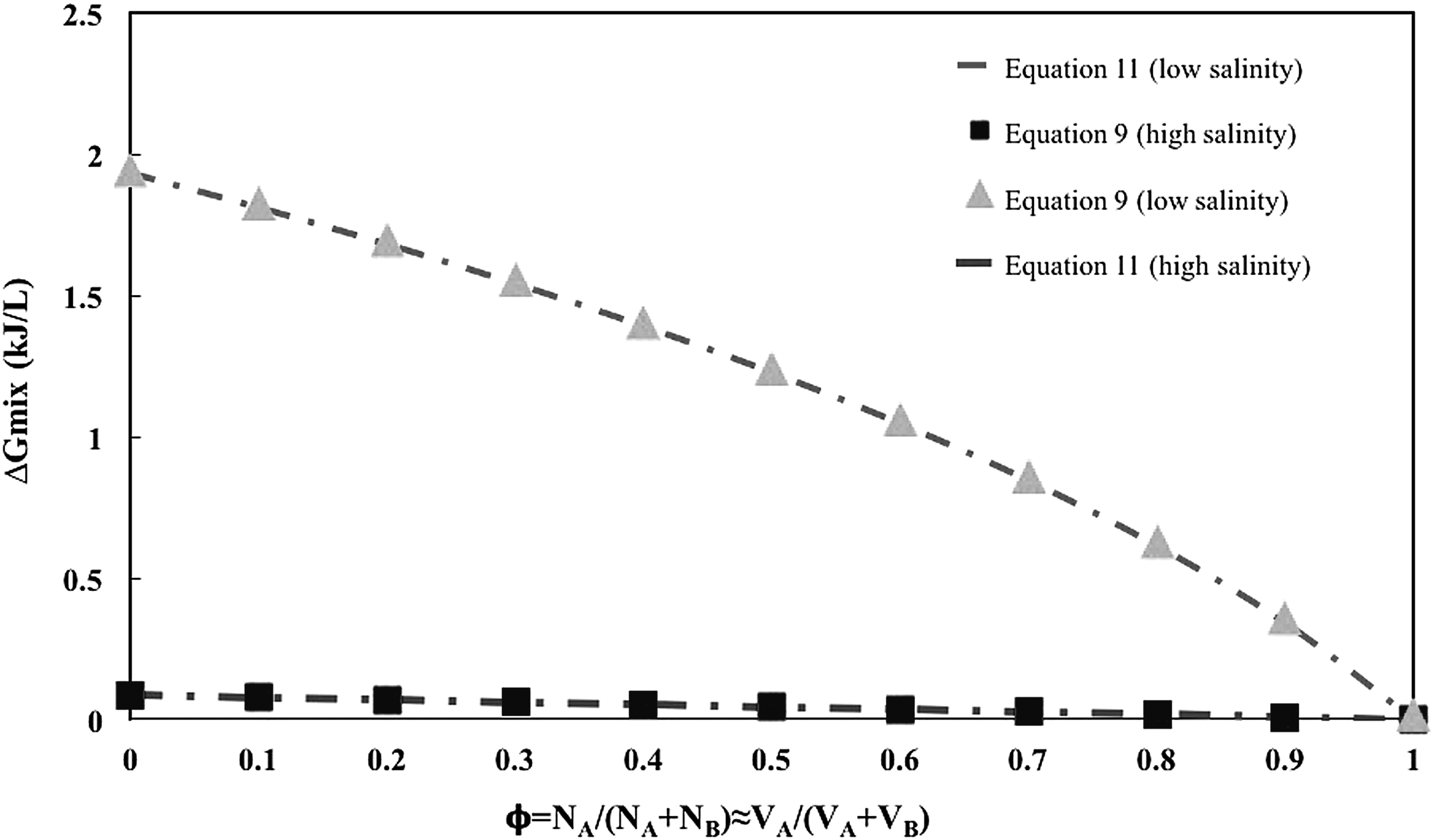
Gibbs free energy of mixing, ΔG_mix,VA, as a function of the mole fraction of the Sal River (A) to both the river water and seawater (A and B), Ф.

FIG. 5.

Gibbs free energy of mixing, ΔG_mix,VA, as a function of the mole fraction of the Chapora River (A) to both the river water and seawater (A and B), Ф.

FIG. 6.

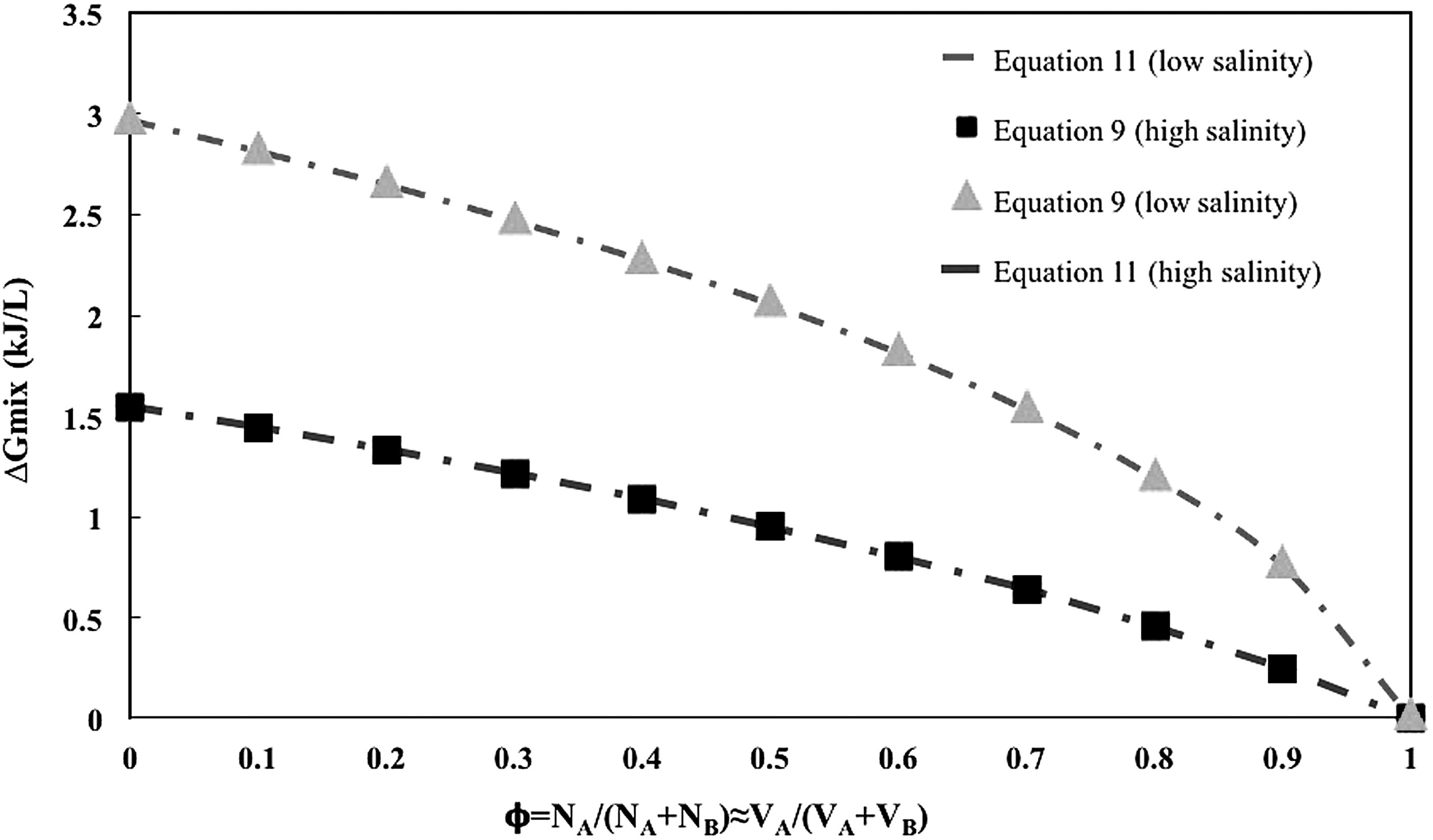
Gibbs free energy of mixing, ΔG_mix,VA, as a function of the mole fraction of the Bicholim River (A) to both the river water and seawater (A and B), Ф.

FIG. 7.

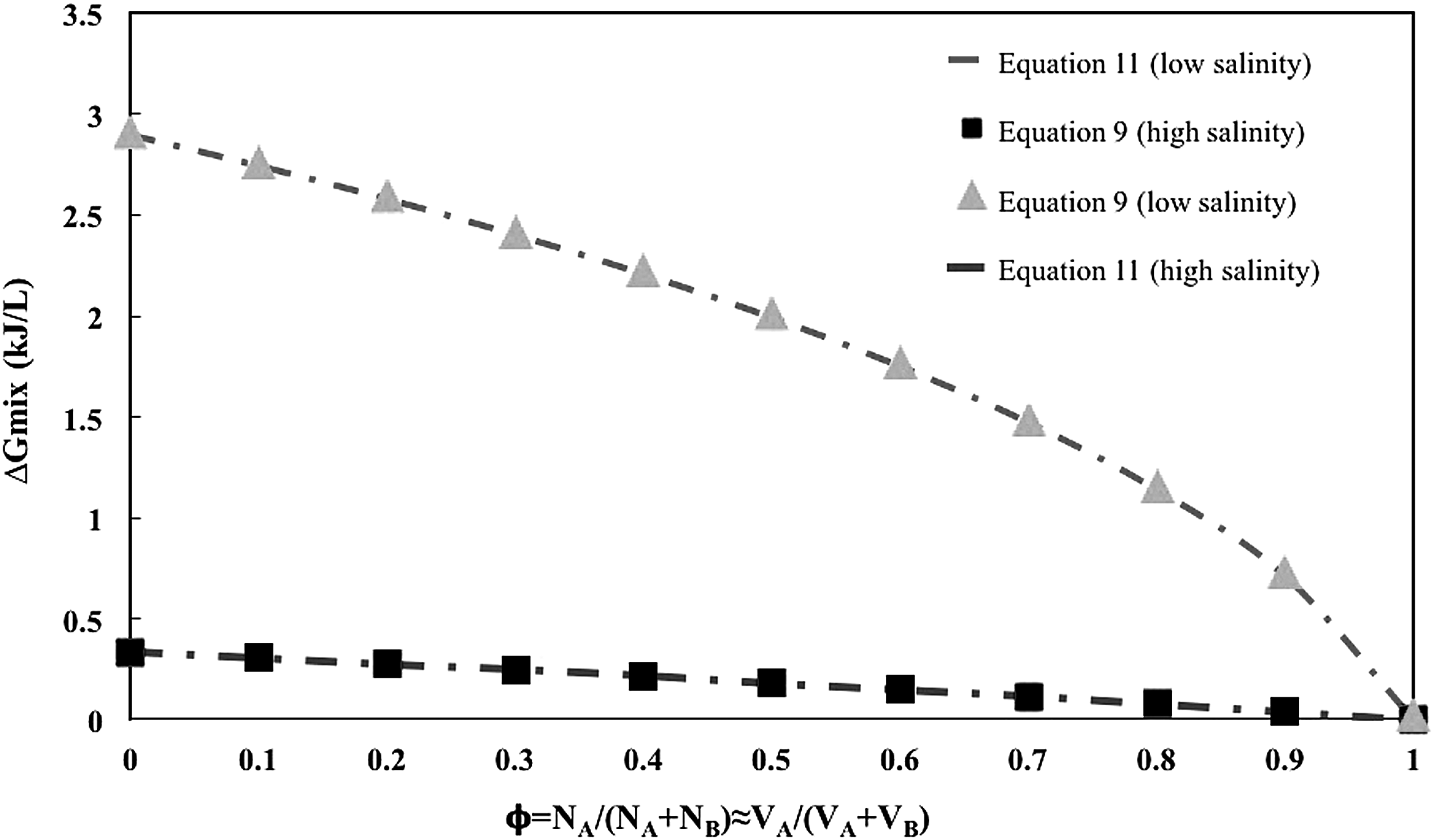
Gibbs free energy of mixing, ΔG_mix,VA, as a function of the mole fraction of the Cumbarjhua River (A) to both the river water and seawater (A and B), Ф.

FIG. 8.

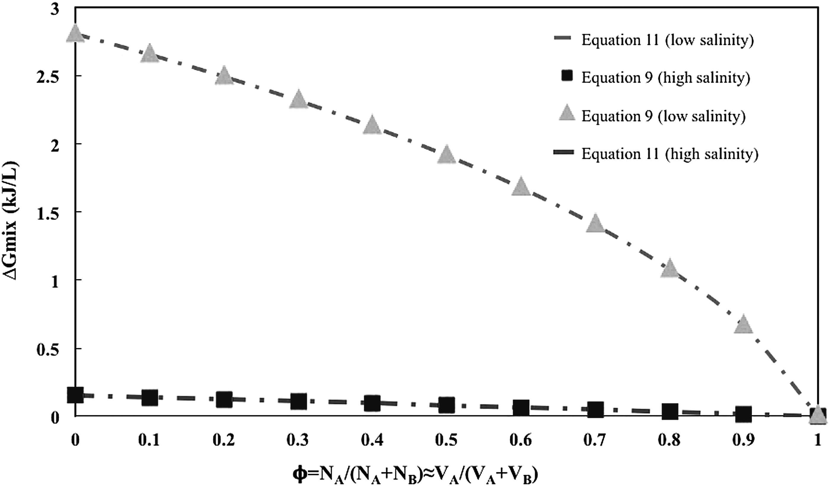
Gibbs free energy of mixing, ΔG_mix,VA, as a function of the mole fraction of the Zuari River (A) to both the river water and seawater (A and B), Ф.

FIG. 9.

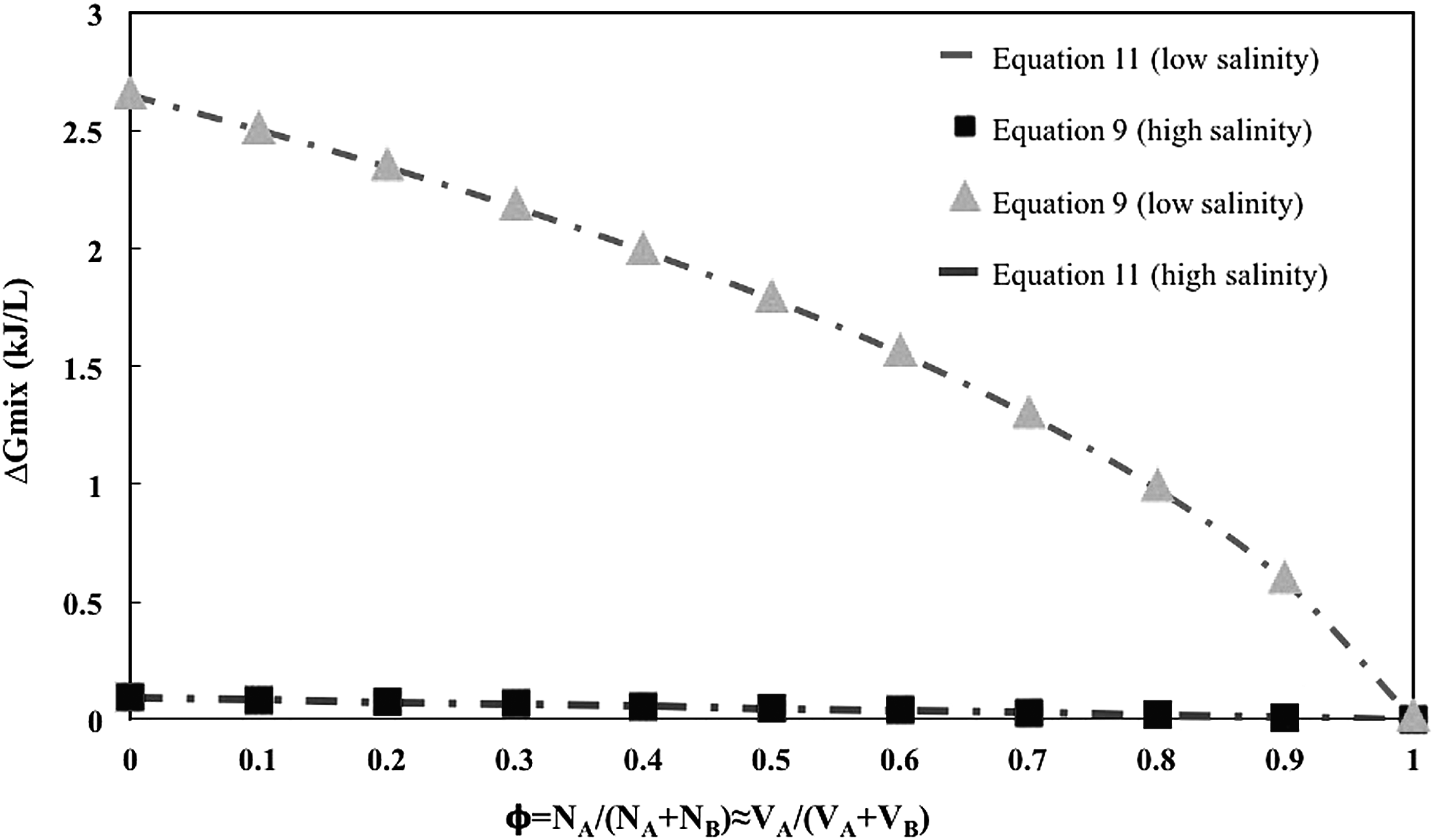
Gibbs free energy of mixing, ΔG_mix,VA, as a function of the mole fraction of the Tiracol River (A) to both the river water and seawater (A and B), Ф.

The Mandovi river (Fig. 3) has the highest ΔG_mix values of 2.7 kJ/L and lowest one being almost 0.01 kJ/L. Sal river (Fig. 4) has the lowest and highest ΔG_mix values of 0.1 kJ/Land 1.9 kJ/L, respectively. Similar values for Chapora river (Fig. 5) are 0.1 kJ/L and 2.8 kJ/L, respectively. Bicholim river (Fig. 6) has the highest value at 2.8 kJ/L and lowest value at 1.5 kJ/L. Cumbharjua canal (Fig. 7) has highest value of ΔG_mix as 2.7 kJ/L and lowest value of 0.4 kJ/L. Similar values for Zuari river (Fig. 8) are 2.8 kJ/L and 0.2 kJ/L. Lastly, Tiracol river (Fig. 9) has the highest Gibbs free energy of mixing at 2.6 kJ/L and lowest at 0.1 kJ/L. Another aspect to note from the above observations is that the performance of Equations (9) and (11) are identical in predicting the ΔG_mix values. This is because \documentclass{aastex}\usepackage{amsbsy}\usepackage{amsfonts}\usepackage{amssymb}\usepackage{bm}\usepackage{mathrsfs}\usepackage{pifont}\usepackage{stmaryrd}\usepackage{textcomp}\usepackage{portland, xspace}\usepackage{amsmath, amsxtra}\usepackage{upgreek}\pagestyle{empty}\DeclareMathSizes{10}{9}{7}{6}\begin{document} \begin{align*} \ln \left( {{ \gamma _{s , M}}{c_M}} \right) = \ln \left( {{ \gamma _{s , M}}} \right) + \ln \left( {{c_M}} \right) \approx \ln \left( {{c_M}} \right) \tag{12} \end{align*} \end{document}

This can be illustrated with the fact that for seawater (600 mM), ln(c_M) = ln (0.0107) = −4.54. While, ln(γ_s,M) = ln (0.672) = −0.42 (Yip and Elimelech, 2012). Thus, there is 1 order of magnitude difference between the values. Hence Equation (12) is valid and this explains the accuracy of prediction of both Equations (9) and (11). From the figures it is evident that the maximum Gibbs energy of mixing for any river is obtained when φ = 0, that is, the case when infinitesimal amount of river water mixes with seawater of infinite volume. The highest value of energy of mixing for each river is tabulated in Table 3.

Table 3.

Highest Energy of Mixing and Maximum Fluctuation in Mixing Energies for Various Rivers in Goa

Sl. No.	Rivers	Highest energy of mixing (kJ/L)	Highest energy of mixing (kWh/m ³ )	Maximum fluctuation in mixing energy (kWh/m ³ )
1	Selaulim (Sanguem)	2.8 ± 0.1	0.77 ± 0.02	0.60 ± 0.02
2	Mandovi (Panjim)	2.7 ± 0.2	0.75 ± 0.04	0.73 ± 0.04
3	Sal (Mobor)	1.9 ± 0.1	0.52 ± 0.02	0.50 ± 0.02
4	Chapora (Siolim bridge)	2.8 ± 0.1	0.77 ± 0.02	0.72 ± 0.02
5	Bicholim (Barazan Nagar)	2.8 ± 0.1	0.77 ± 0.02	0.36 ± 0.02
6	Cumbharjua canal (Corlim)	2.7 ± 0.2	0.75 ± 0.04	0.66 ± 0.02
7	Zuari (Cortalim)	2.8 ± 0.2	0.77 ± 0.04	0.72 ± 0.02
8	Tiracol (Keri, Pernem)	2.6 ± 0.1	0.72 ± 0.02	0.7 ± 0.02

It is evident that 2.8 kJ/L or 0.77 kWh/m³ is the highest average energy of mixing (HAEM) expected from the mixing of rivers and saline bodies like oceans. This corresponds to the observations made earlier (Gadgil, 2003; Semiat, 2008; Elimelech and Philip, 2011; Yip and Elimelech, 2012). It must be noted here that the minimum energy of desalination (W) is obtained from the theoretical Gibbs free energy of mixing formulation (Semiat, 2008): \documentclass{aastex}\usepackage{amsbsy}\usepackage{amsfonts}\usepackage{amssymb}\usepackage{bm}\usepackage{mathrsfs}\usepackage{pifont}\usepackage{stmaryrd}\usepackage{textcomp}\usepackage{portland, xspace}\usepackage{amsmath, amsxtra}\usepackage{upgreek}\pagestyle{empty}\DeclareMathSizes{10}{9}{7}{6}\begin{document} \begin{align*} W = \int \limits_{{n_1}}^{{n_2}} { \Delta Gdn = \int \limits_{{n_1}}^{{n_2}} {RT \ln { \gamma _w}dn} } = \int \limits_{{n_1}}^{{n_2}} {RT \ln {p \over {{p_0}}}dn} \\= {{0.296T} \over {100 - {n_2}}} \int \limits_{{n_2}}^{100} { \log {p \over {{p_0}}}dn} \tag{13} \end{align*} \end{document}

where, 1 and 2 represents the two states of before and after desalination, n is the moles of water, and p represents the water vapor pressure when assumed as ideal gas. For 50% recovery W becomes 1.09 kWh/m³, which also represents the minimum energy required for desalination. Now, the mixing Gibbs energy of the rivers like Selaulim, Chapora, Bicholim, and Zuari yields HAEM of 0.77 kWh/m³, which is similar to that of minimum energy of desalination of seawater at 0% recovery. This is consistent with reversible thermodynamics in the sense that the minimum energy of separation is equal in magnitude but opposite in sign to the energy of mixing due to mixing.

Interestingly, the present analysis brings out lot of important aspects. The Gibbs free energy of mixing evolved from river and seawater mixing can be used for purposes like PRO for power generation. However, the important question to be asked are as follows: (i) what is the desired salinity level for such energy output, (ii) how to choose location for such plants, and (iii) what is the seasonal variation of energy output expected from such installations?

It is evident that the upper limit of such mixing process is of course 0.77 kWh/m³ as this includes the limit of river water (low salinity) mixing with seawater, which has a fixed salinity. The river water salinity levels cannot go any lower neither can one expect the salinity of seawater to increase, only two possibilities that can yield higher values than 0.77 kWh/m³. However, the other aspect to note is that this represents the thermodynamic limit and real-life power generation from such mixing using technologies like PRO can never attain this value due to irreversibilities. This constraint is imposed by the second law of thermodynamics where entropy generation makes it impossible to carry out processes operating within finite driving forces without losses. These losses never allow any practical process to attain the limits set by Gibbs free energy. Thus, it is clear that highest power that can be extracted from salinity driven mixing is set by the Gibbs energy of mixing values. Having established the upper limits of energy generation, it is important to explore decision-making issues like geographical location of such plants.

From Table 3, it can be observed that Selaulim, Chapora, Bicholim, and Zuari have HAEM values (0.77 kWh/m³). They are followed by Mandovi and Cumbarjhua (0.75 kWh/m³) and Tiracol (0.72 kWh/m³) and Sal (0.5 kWh/m³). It is also clear that Selaulim, Chapora, Bicholim, and Zuari all have the same mixing energies, but due to the seasonal fluctuation in salinities, the reduction in values (difference between maximum and minimum values of energy of mixing) among the four is highest for Zuari and Chapora and lowest for Bicholim. This puts Bicholim at an advantage over the rest three but another aspect that must be considered is that volumetric flow rate of rivers. Zuari has highest volumetric flow among the three and obviously higher than Bicholim so even if seasonal fluctuations put Zuari at a disadvantage, yet due to high volume, energy generation will be significantly higher. Other aspect to be considered is that while taking decisions on location, seawater intrusion should also be taken into account. Seawater intrusion has resulted in river waters turning brackish and as is evident from this study that higher salinity hinders evolution of energy. Thus, geographical location of PRO plants can be decided on upon such analysis. Choice of rivers and choice of location along the river, are two important decision-making parameters for PRO installations.

For PRO plants, there can be two variables that affect the power generation, and they are the volumetric flow rate of rivers and salinity of the river water. The seasonal dependent volumetric flow rates of river is a parameter that can be controlled in the PRO plant design as peak and average flow rates can be assumed for piping design and operation. Based on this study, the only variable that cannot be controlled is the seasonal salinity levels in the rivers. Now, it is important to understand the implication of such salinity variations in a PRO unit. It is reported that power density (obtained from PRO) can be estimated as follows: \documentclass{aastex}\usepackage{amsbsy}\usepackage{amsfonts}\usepackage{amssymb}\usepackage{bm}\usepackage{mathrsfs}\usepackage{pifont}\usepackage{stmaryrd}\usepackage{textcomp}\usepackage{portland, xspace}\usepackage{amsmath, amsxtra}\usepackage{upgreek}\pagestyle{empty}\DeclareMathSizes{10}{9}{7}{6}\begin{document} \begin{align*} \dot W = {J_w} \Delta P = {L_P} \Delta P \left( { \Delta \pi - \Delta P} \right) \tag{14} \end{align*} \end{document}

where, \documentclass{aastex}\usepackage{amsbsy}\usepackage{amsfonts}\usepackage{amssymb}\usepackage{bm}\usepackage{mathrsfs}\usepackage{pifont}\usepackage{stmaryrd}\usepackage{textcomp}\usepackage{portland, xspace}\usepackage{amsmath, amsxtra}\usepackage{upgreek}\pagestyle{empty}\DeclareMathSizes{10}{9}{7}{6}\begin{document} $$\dot W$$ \end{document} is the power density (W/m²), L_P is the system permeability (L/m²-hr-bar), \documentclass{aastex}\usepackage{amsbsy}\usepackage{amsfonts}\usepackage{amssymb}\usepackage{bm}\usepackage{mathrsfs}\usepackage{pifont}\usepackage{stmaryrd}\usepackage{textcomp}\usepackage{portland, xspace}\usepackage{amsmath, amsxtra}\usepackage{upgreek}\pagestyle{empty}\DeclareMathSizes{10}{9}{7}{6}\begin{document} $$\Delta \pi$$ \end{document} and \documentclass{aastex}\usepackage{amsbsy}\usepackage{amsfonts}\usepackage{amssymb}\usepackage{bm}\usepackage{mathrsfs}\usepackage{pifont}\usepackage{stmaryrd}\usepackage{textcomp}\usepackage{portland, xspace}\usepackage{amsmath, amsxtra}\usepackage{upgreek}\pagestyle{empty}\DeclareMathSizes{10}{9}{7}{6}\begin{document} $$\Delta P$$ \end{document} are the net difference in osmotic pressure and hydraulic pressure, respectively (in bars), with \documentclass{aastex}\usepackage{amsbsy}\usepackage{amsfonts}\usepackage{amssymb}\usepackage{bm}\usepackage{mathrsfs}\usepackage{pifont}\usepackage{stmaryrd}\usepackage{textcomp}\usepackage{portland, xspace}\usepackage{amsmath, amsxtra}\usepackage{upgreek}\pagestyle{empty}\DeclareMathSizes{10}{9}{7}{6}\begin{document} $$\Delta P = 15$$ \end{document} bars. Equation (14) is plotted (Fig. 10) and the variation of L_P against power density for various values of \documentclass{aastex}\usepackage{amsbsy}\usepackage{amsfonts}\usepackage{amssymb}\usepackage{bm}\usepackage{mathrsfs}\usepackage{pifont}\usepackage{stmaryrd}\usepackage{textcomp}\usepackage{portland, xspace}\usepackage{amsmath, amsxtra}\usepackage{upgreek}\pagestyle{empty}\DeclareMathSizes{10}{9}{7}{6}\begin{document} $$\Delta \pi$$ \end{document} . It is to be noted that the axes (Fig. 10) begins from 3.5 W/m² and this is because to make PRO commercially viable and attractive, the energy density has to be maintained somewhere between 4 and 6 (Sharif et al., 2014). Important observations can be made from the figure and especially in context with the current effort. For a value of \documentclass{aastex}\usepackage{amsbsy}\usepackage{amsfonts}\usepackage{amssymb}\usepackage{bm}\usepackage{mathrsfs}\usepackage{pifont}\usepackage{stmaryrd}\usepackage{textcomp}\usepackage{portland, xspace}\usepackage{amsmath, amsxtra}\usepackage{upgreek}\pagestyle{empty}\DeclareMathSizes{10}{9}{7}{6}\begin{document} $$\Delta \pi$$ \end{document} = 20 bars, L_P = 1.8 L/m²-hr-bar, power density is 4 W/m². However, when \documentclass{aastex}\usepackage{amsbsy}\usepackage{amsfonts}\usepackage{amssymb}\usepackage{bm}\usepackage{mathrsfs}\usepackage{pifont}\usepackage{stmaryrd}\usepackage{textcomp}\usepackage{portland, xspace}\usepackage{amsmath, amsxtra}\usepackage{upgreek}\pagestyle{empty}\DeclareMathSizes{10}{9}{7}{6}\begin{document} $$\Delta \pi$$ \end{document} = 30 bars, L_P = 0.6 L/m²-hr-bar for the same power density.

FIG. 10.

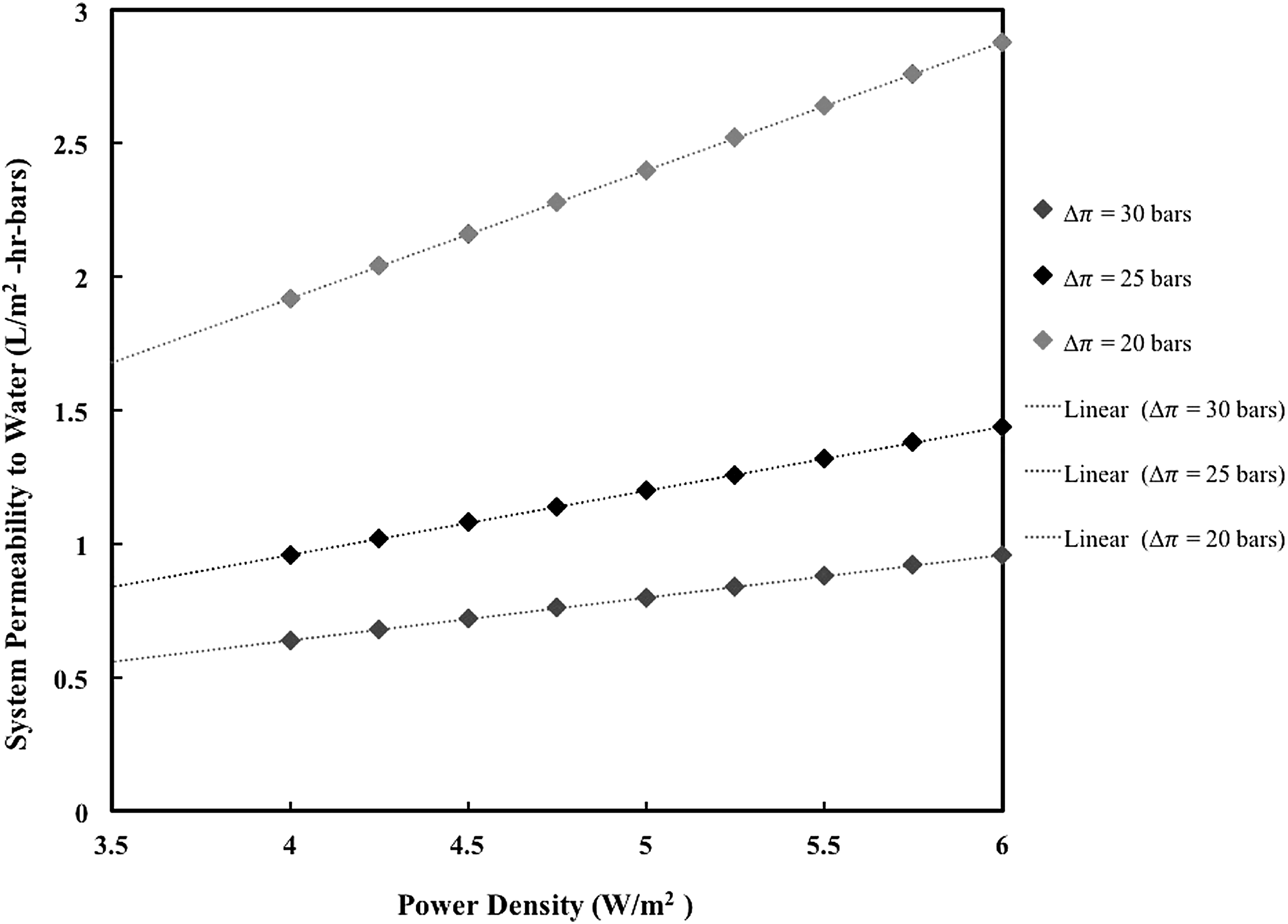
Variation of system permeability to water (L_p) with the power density ( \documentclass{aastex}\usepackage{amsbsy}\usepackage{amsfonts}\usepackage{amssymb}\usepackage{bm}\usepackage{mathrsfs}\usepackage{pifont}\usepackage{stmaryrd}\usepackage{textcomp}\usepackage{portland, xspace}\usepackage{amsmath, amsxtra}\usepackage{upgreek}\pagestyle{empty}\DeclareMathSizes{10}{9}{7}{6}\begin{document} $$\dot W$$ \end{document} ) or different values of osmotic pressure (Δπ).

This is a significant finding, since it demonstrates that for a difference of 10 bars in osmotic pressure differential, the membrane permeability has to be increased almost three-folds. Similarly, for same power density (5 W/m²) for \documentclass{aastex}\usepackage{amsbsy}\usepackage{amsfonts}\usepackage{amssymb}\usepackage{bm}\usepackage{mathrsfs}\usepackage{pifont}\usepackage{stmaryrd}\usepackage{textcomp}\usepackage{portland, xspace}\usepackage{amsmath, amsxtra}\usepackage{upgreek}\pagestyle{empty}\DeclareMathSizes{10}{9}{7}{6}\begin{document} $$\Delta \pi$$ \end{document} = 30 bars, L_P = 0.6 L/m²-hr-bar, whereas for \documentclass{aastex}\usepackage{amsbsy}\usepackage{amsfonts}\usepackage{amssymb}\usepackage{bm}\usepackage{mathrsfs}\usepackage{pifont}\usepackage{stmaryrd}\usepackage{textcomp}\usepackage{portland, xspace}\usepackage{amsmath, amsxtra}\usepackage{upgreek}\pagestyle{empty}\DeclareMathSizes{10}{9}{7}{6}\begin{document} $$\Delta \pi$$ \end{document} = 20 bars L_P = 2.4 L/m²-hr-bar. Thus, to maintain the same power density the permeability has to increase four-folds for a pressure differential of 10 bars between osmotic and hydraulic pressures. This depicts the fact that due to significant difference between \documentclass{aastex}\usepackage{amsbsy}\usepackage{amsfonts}\usepackage{amssymb}\usepackage{bm}\usepackage{mathrsfs}\usepackage{pifont}\usepackage{stmaryrd}\usepackage{textcomp}\usepackage{portland, xspace}\usepackage{amsmath, amsxtra}\usepackage{upgreek}\pagestyle{empty}\DeclareMathSizes{10}{9}{7}{6}\begin{document} $$\left( { \Delta \pi - \Delta P} \right)$$ \end{document} the membrane requirement changes and obviously associated design too has to alter. Thus, the rivers under investigation in this study have osmotic pressure of around 27 bars. If seasonal variations in salinity are not taken into account then PRO plant designs would change significantly and the same plant that would be operational in monsoon might not be deemed suitable for the summer months. More importantly, it can be inferred from the graph that as the osmotic pressure differential decreases the system permeabilities increase and as it approaches the value of \documentclass{aastex}\usepackage{amsbsy}\usepackage{amsfonts}\usepackage{amssymb}\usepackage{bm}\usepackage{mathrsfs}\usepackage{pifont}\usepackage{stmaryrd}\usepackage{textcomp}\usepackage{portland, xspace}\usepackage{amsmath, amsxtra}\usepackage{upgreek}\pagestyle{empty}\DeclareMathSizes{10}{9}{7}{6}\begin{document} $$\Delta P = 15$$ \end{document} bars the requirement experiences a huge jump. This is consistent with the concept of equilibrium since at osmotic pressure differentials approaching hydraulic pressure there will be no flux and system permeability requirement will be infinity.

With this discussion, it is important to delve a little further into understanding the implication of such saline river waters in PRO processes. With reported values of salinity of Zuari river (Manoj and Unnikrishnan, 2009) from the confluence point (in kms) the Gibbs energy of mixing with seawater was calculated. It must be noted that this is only a representative calculation (with static head = 8.9 m) and a possible strategy that can be adopted for such analysis. Now, to determine the geographical location for a PRO plant, the position should be such that Gibbs energy of mixing yields high values with minimum pumping requirements. It can be assumed that the PRO plant can be placed close to either river water or the seawater and pump the other stream. Thus, Fig. 11 shows the pumping requirements (kWh/m³) of a single stream and Gibbs energy of mixing (kWh/m³) as function of distance from the confluence.

FIG. 11.

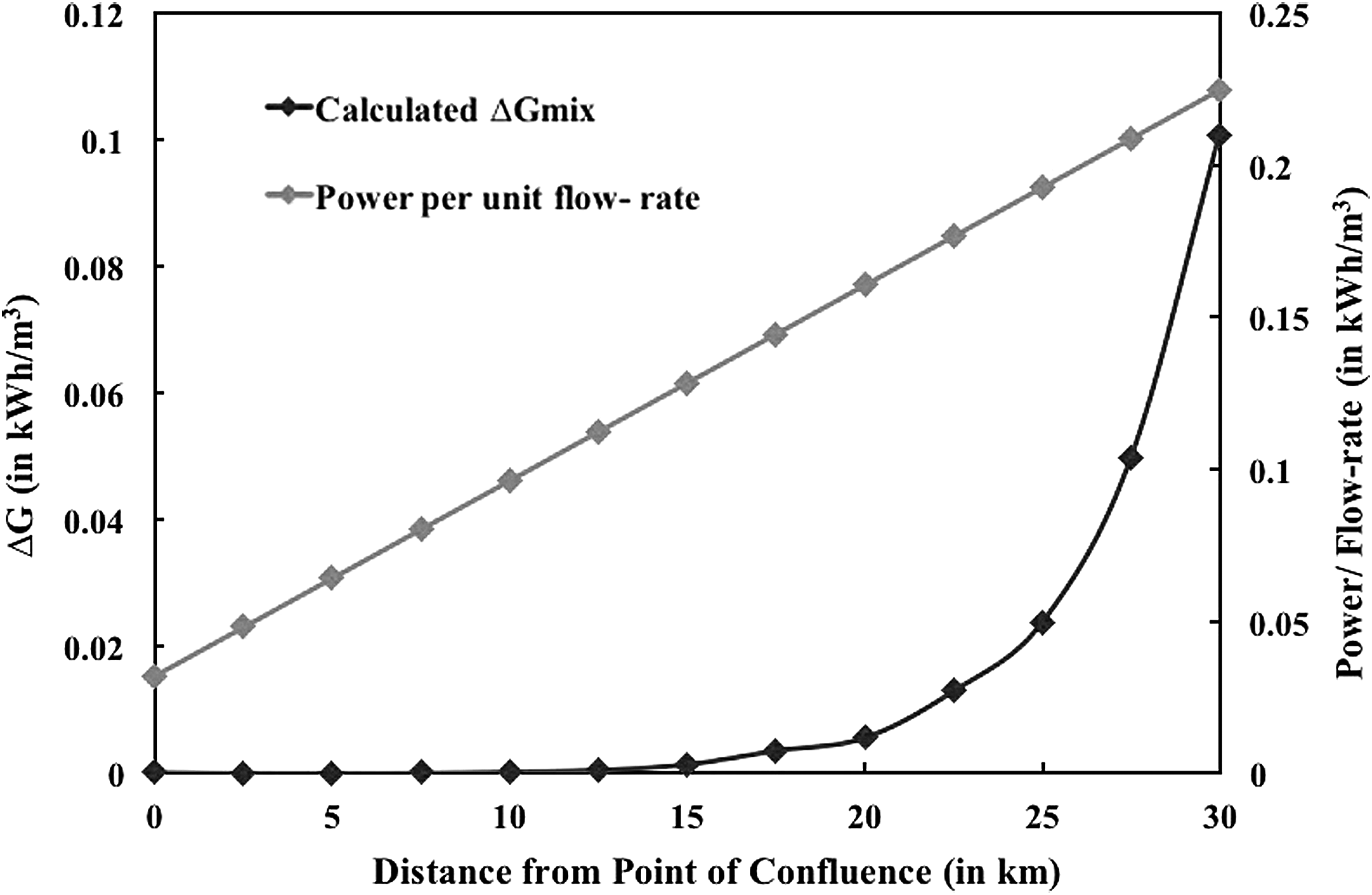
Variation of ΔG_mix with power per unit flow rate (both in kWh/m³).

Based on the understanding that higher salinity of rivers is detrimental to the mixing energy obtained, installation of a PRO plant downstream is made significantly challenging as a result of seasonal variation in river water salinities. It is evident that while the maximum Gibbs energy of mixing is obtained at around 26 km from the confluence point but the pumping requirement for the water imposes a great challenge toward the feasibility of the process. Thus, there is a clear necessity toward developing strategies to address such issues of salinities in estuarine systems for generation of power through PRO for a guaranteed rated power output throughout the year. Overall, salinity driven power generation can be the future for regions like Goa and countries like India and can be the future of sustainable technologies with help of proper strategies.

In this context, it was also important to understand the variation of temperature effects on mixing energies. Due to climate change, hydrological and thermal regimes of rivers are expected to change. This will have direct consequences for freshwater ecosystems, water quality, and human water use (van Vliet et al., 2013). With respect to PRO energy generation, analysis has been done on the basis of data obtained (Qasim and Gupta, 1981), which includes temperature data for three major rivers in Goa, Zuari, Mandovi, and Cumbharjua Canal, as calculated in 1981.

The variation of temperature on Gibbs free energy of mixing has been studied for three rivers, namely Zuari, Mandovi, and Cumbharjua Canal, taking data from literature for the temperature and salinity in 1981, against data taken during the 2014–2015 period from Goa State Pollution Control Board Annual Report. The variation in salinity for the 4 months- January, February, March, and April has been taken as constant since there is not much variation, as is evident from literature data. The temperature of the respective year has been used for calculation of the Gibbs free energy of mixing. Finally, the variation has been obtained as the absolute value of the difference of the Gibbs free energy of mixing, as calculated for the salinity corresponding to that year and the standard temperature of 298 K, and that calculated with the reported corresponding salinity and corresponding temperature. The data have been illustrated graphically, in Figs. 12 –14.

FIG. 12.

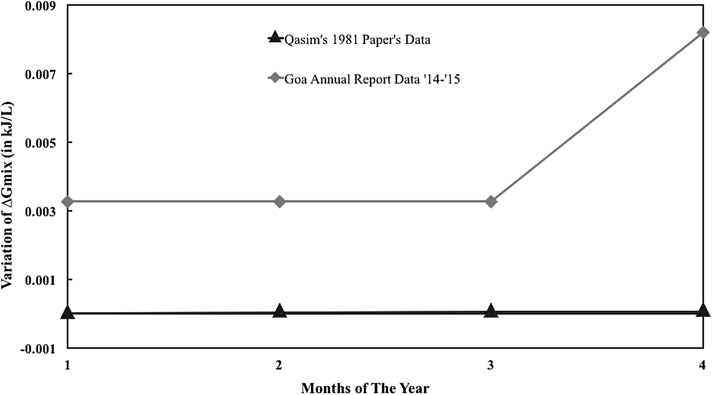
Variation of ΔG_mix,VA with temperature for Zuari at Cortalim, in 1981 and 2014–2015.

FIG. 13.

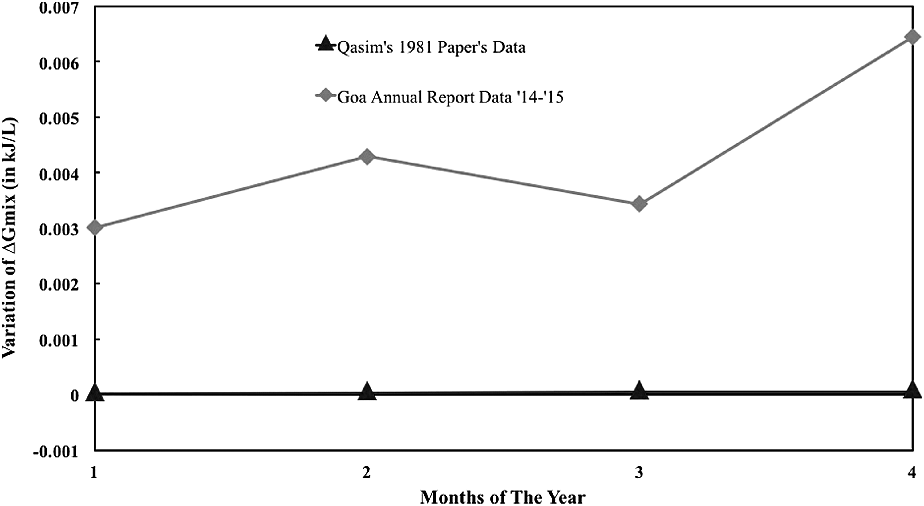
Variation of ΔG_mix,VA with temperature for Mandovi at Panaji, in 1981 and 2014–2015.

FIG. 14.

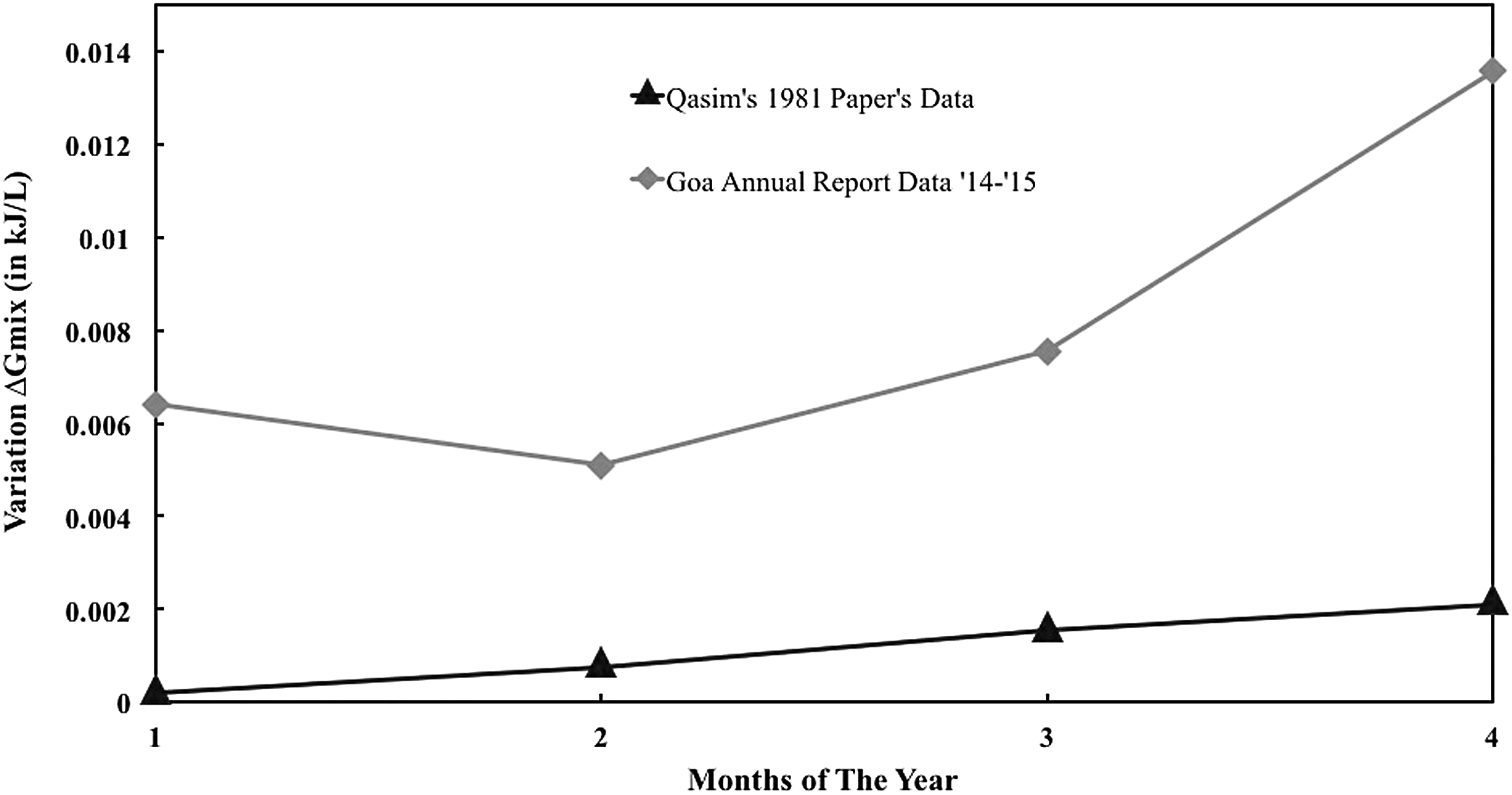
Variation of ΔG_mix,VA with temperature for Cumbharjua Canal at Corlim, in 1981 and 2014–2015.

It is evident that the variation of temperature is significant in the period of 2014–2015, as compared to that as calculated for the year of 1981. This is the case for all the three rivers under study. The overall variation in temperature for the 12 months is approximately 4–5°C, for both the periods. However, an interesting observation is that the average temperatures throughout both the 12-month periods under study vary by 1.2°C, with the average temperature being higher in 2014–2015, than in 1981. This is a matter of concern and points toward the global warming phenomenon, which indicates that it is of utmost importance to look toward the renewable sources of energy generation, such as the discussed PRO.

In Fig. 12, the highest variation in Gibbs energy of mixing from that calculated at 298 K is 0.008 kJ/L, and this is based on the Goa Annual River Report Data for the 2014–2015 period. The same is as low as the obtained 0.00007 kJ/L for the 1981 data.

Thus, we can clearly infer that the temperature variation is significant in the period of 2014–2015. The same can be inferred from the Figs. 13 and 14 for the Mandovi and Cumbharjua Canal Rivers respectively.

What can be directly observed is that the average energy of mixing has increased over the past three decades, since the Free Energy of Mixing in the year 2014–2015 is on average turning out to be more than that in 1981. Twenty-five years of extensive water temperature data show regionally coherent warming to have occurred in Alpine rivers and streams at all altitudes, reflecting changes in regional air temperature (Hansen et al., 2006). Although beneficial for the overall aim of achieving as high a Gibbs Free Energy of Mixing as possible, it is reasonable to infer that the rising temperatures has resulted from global warming, and as has been confirmed in the past, it is a matter of concern for mankind.

Conclusion

In this article, the authors have investigated the effect of salinity variation in rivers and the possible effect of the same on PRO process for power generation. The article sheds light on the detrimental effect of salinity increase in rivers, which can actually challenge processes like PRO and as an example eight major rivers of Goa have been analyzed for the same. It has been shown that while in the rainy season the Gibbs energy of mixing of rivers like Zuari (and hence potential power generation) can be maximum the same almost reduces to zero during the summer period. This in turn can have a detrimental effect on the design of PRO units, as larger membrane permeabilities will be required to meet the same power densities for the increased salinities. This is impossible since different membrane modules will be required for different seasons and is economically and operationally infeasible. Importantly, the geographical location of such plants also impose a challenge since salinity ingress increase pumping requirements and an optimum has to be identified with regards to Gibbs energy of mixing and pumping powers. Overall, the article is focused on identifying challenges associated with practical implementation of PRO in rivers where salinity variations are large and therefore technological solutions are necessary to address the same.

Footnotes

Acknowledgments

Anirban would like to thank the Research Initiation Grant (BPGC/RIG/2017–2018, dt. 01/0/2017) and OPERA award (FR/SCM/230117/CHE, dt. 19/08/2017) by BITS Pilani Goa for carrying out the work.

Author Disclosure Statement

No competing financial interests exist.

References

Achilli

, and Childress

A.E.

(2010). Pressure retarded osmosis: From the vision of Sidney Loeb to the first prototype installation. Desalination. 261, 205.

Achilli

, Cath

T.Y.

, and Childress

A.E.

(2009). Power generation with pressure retarded osmosis: An experimental and theoretical investigation. J. Membr. Sci., 343, 42.

Dai

, and Trenberth

K.E.

(2002). Estimates of freshwater discharge from continents: Latitudinal and seasonal variations. J. Hydrometeorol., 3, 660.

Elimelech

, and Phillip

W.A.

(2011). The Future of Seawater Desalination: Energy, Technology, and the Environment. Science. 333, 712.

Gadgil

(2003). The Indian monsoon and its variability, Annu. Rev. Earth Planet. Sci., 31, 429.

Hansen

, Sato

, Ruedy

, Lo

, Lea

D.W.

, and Medina-Elizade

(2006). Global temperature change. Proc. Natl. Acad. Sci. U.S.A., 103, 14288.

Hatzell

M.C.

, Cusick

R.D.

, and Logan

B.E.

(2014). Capacitive mixing power production from salinity gradient energy enhanced through exoelectrogen-generated ionic currents. Energy Environ. Sci., 7, 1159.

Jakhrani

A.Q.

, Samo

S.R.

, Sobuz

H.R.

, Uddin

M.A.

, Ahsan

M.J.

, and Hasan

N.M.S.

(2012). Assessment of Dissolved Salts Concentration of Seawater in the Vicinity of Karachi. Intern. J. Struct. Civil Engg., 1, 61.

Klaysom

, Cath

T.Y.

, Depuydt

, and Vankelecom

I.F.

(2013). Forward and pressure retarded osmosis: Potential solutions for global challenges in energy and water supply. Chem. Soc. Rev., 42, 6959.

10.

Kumar

, Singh

R.D.

, and Sharma

K.D.

(2005). Water resources of India. Curr. Sci., 794.

11.

Kurihara

, and Hanakawa

(2013). Mega-ton Water System: Japanese national research and development project on seawater desalination and wastewater reclamation. Desalination. 308, 131.

12.

Lin

, Straub

A.P.

, and Elimelech

(2014). Thermodynamic limits of extractable energy by pressure retarded osmosis. Energy Environ. Sci., 7, 2706.

13.

Manoj

N.T.

, and Unnikrishnan

A.S.

(2009). Tidal circulation and salinity distribution in the Mandovi and Zuari estuaries: Case study. J. Waterw. Port Coast. Ocean Eng., 135, 278.

14.

McGinnis

R.L.

, and Elimelech

(2008). Global challenges in energy and water supply: The promise of engineered osmosis, Environ. Sci. Technol., 42, 8625.

15.

Mistry

K.H.

, Hunter

H.A.

, and Lienhard

J.H.V.

(2013). Effect of composition and nonideal solution behavior on desalination calculations for mixed electrolyte solutions with comparison to seawater. Desalination. 318, pp.34–47.

16.

Mistry

K.H.

, and Lienhard

J.H.V.

(2013). Effect of nonideal solution behavior on desalination of a sodium chloride solution and comparison to seawater. J. Energy Res. Technol., 135, 042003.

17.

Naylor

R.L.

(1996). Energy and resource constraints on intensive agricultural production. Annu. Rev. Energy Env., 21, 99.

18.

Noronha

(2015). Goa State Pollution Control Board, Annual Report 2014–2015.

19.

Parker

V.B.

, and États-Unis. National Bureau of Standards, 1965. Thermal Properties of Aqueous Uni-Univalent Electrolytes (Vol. 2). Washington, DC: US Government Printing Office.

20.

Pattle

R.E.

(1954). Production of electric power by mixing fresh and salt water in the hydroelectric pile. Nature. 174, 660.

21.

Pitzer

K.S.

, Peiper

J.C.

, and Busey

R.H.

(1984). Thermodynamic properties of aqueous sodium-chloride solutions. J. Phys. Chem. Ref. Data., 13, 1.

22.

Qasim

S.Z.

, and Gupta

R.S.

(1981). Environmental characteristics of the Mandovi-Zuari estuarine system in Goa. Estuar. Coast. Mar. Sci., 13, 557.

23.

Ramon

G.Z.

, Feinberg

B.J.

, and Hoek

E.M.

(2011). Membrane-based production of salinity-gradient power. Energy Environ. Sci., 4, 4423.

24.

Rica

R.A.

, Ziano

, Salerno

, Mantegazza

, van Roij

, and Brogioli

(2013). Capacitive mixing for harvesting the free energy of solutions at different concentrations. Entropy. 15, 1388.

25.

Robinson

R.A.

, and Stokes

R.H.

(2002). Electrolyte Solutions, 2nd rev. ed. Mineola, NY: Dover Publications, 571, p xv.

26.

Semiat

(2008). Energy issues in desalination processes. Environ. Sci. Technol., 42, 8193–8201.

27.

Senthil Kumar

A.R.

, Sudheer

K.P.

, Jain

S.K.

, and Agarwal

P.K.

(2005). Rainfall‐runoff modelling using artificial neural networks: Comparison of network types, Hydrol. Process. 19, 1277.

28.

Sharif

A.O.

, Merdaw

A.A.

, Aryafar

, and Nicoll

(2014). Theoretical and experimental investigations of the potential of osmotic energy for power production. Membranes. 4, 447.

29.

Sharif

A.O.

, Merdaw

A.A.

, Al-Bahadili

, Al-Taee

, Al-Aibi

, Rahal

, and Derwish

G.A.W.

(2009). A new theoretical approach to estimate the specific energy consumption of reverse osmosis and other pressure-driven liquid-phase membrane processes. Desalin. Water Treat., 3, 111.

30.

Shetye

S.R.

, Dileep Kumar,M., and Shankar

(2007). The Mandovi and Zuari Estuaries. Goa, India: National Institute of Oceanography. p. 145.

31.

Smalley

R.E.

(2005). Future global energy prosperity: The terawatt challenge. MRS Bulletin. 30, 412.

32.

Smith

J.M.

, Van Ness

H.C.

, and Abbott

M.M.

(2005). Introduction to Chemical Engineering Thermodynamics. New York: McGraw-Hill.

33.

Straub

A.P.

, Deshmukh

, and Elimelech

(2016). Pressure-retarded osmosis for power generation from salinity gradients: Is it viable?. Energy Environ. Sci., 9, 31.

34.

Suprit

, Shankar

, Venugopal

, and Bhatkar

N.V.

(2012). Simulating the daily discharge of the Mandovi River, west coast of India. Hydrol. Sci. J., 57, 686.

35.

Van Vliet

M.T.H.

, Franssen

W.H.P.

, Yearsley

J.R.

, Ludwig

, Haddeland

, Lettenmaier

D.P.

, and Kabat

(2013). Global river discharge and water temperature under climate change. Global Env. Change, 23, 450.

36.

Vitousek

P.M.

, Mooney

H.A.

, Lubchenco

, and Melillo

J.M.

(1997). Human domination of Earth's ecosystems. Science. 277, 494.

37.

Wick

G.L.

(1978). Power from salinity gradients. Energy. 3, 95.

38.

Yip

N.Y.

, and Elimelech

(2012). Thermodynamic and energy efficiency analysis of power generation from natural salinity gradients by pressure retarded osmosis. Environ. Sci. Technol., 46, 5230.