Simplified Process to Determine Rate Constants for Sunlight-Mediated Removal of Trace Organic and Microbial Contaminants in Unit Process Open-Water Treatment Wetlands
Available accessResearch articleFirst published online January, 2019
Simplified Process to Determine Rate Constants for Sunlight-Mediated Removal of Trace Organic and Microbial Contaminants in Unit Process Open-Water Treatment Wetlands
Unit process, open-water (UPOW) treatment wetlands are a unique type of constructed wetlands that are designed to promote photo- and microbiologically mediated natural water treatment processes. A mechanistic understanding of the removal processes for nitrate, trace organic contaminants (TrOCs), and microbial contaminants in UPOW wetlands has been established, and equations have been previously developed to describe removal kinetics. However, the numerical models developed to predict photodegradation rate constants for the removal of TrOC and microbial contaminants involve too many steps to facilitate a practical design approach. In this article, we present a method for predicting rates of phototransformation of representative TrOCs (atenolol, propranolol, sulfamethoxazole, and carbamazepine) and inactivation of microbial indicator organisms (Escherichia coli and MS2) that allows a user to readily design UPOW wetlands to meet different performance goals. Photodegradation rate constants were determined for a range of conditions that influence treatment efficacy (i.e., time of year, pH, latitude, and dissolved organic carbon concentration), and are presented in a series of figures. We illustrate the use of these figures for UPOW wetland design with a representative example of the design process. A spreadsheet containing sample calculations is included in the Supplementary Data.
Introduction
Shallow, unit process, open-water (UPOW) wetlands are natural water treatment systems designed to enhance photo- and microbiologically mediated water treatment processes (Jasper et al., 2013). Treatment processes promoted in open-water wetlands include photolysis and biotransformation of chemical contaminants (including trace organic compounds) (Jasper and Sedlak, 2013; Jasper et al., 2014a; Prasse et al., 2015), photoinactivation of microbial contaminants (Nguyen et al., 2015; Silverman et al., 2015), and microbiological removal of nitrate (e.g., denitrification and anammox) (Jasper et al., 2014b; Jones et al., 2017, 2018). UPOW wetlands have improved treatment efficiency compared with vegetated wetlands given that UPOW wetlands have greater sunlight exposure and are less prone to hydraulic short circuiting (Jasper and Sedlak, 2013; Jasper et al., 2014a, 2014b; Nguyen et al., 2015; Silverman et al., 2015). Given their improved treatment performance, UPOW wetlands are attractive options for the polishing of municipal wastewater effluent, treatment of water from effluent-dominated waterways (e.g., rivers and lakes with a large percentage of their flow or volume consisting of municipal wastewater effluent), and use as the final stage of wastewater treatment pond systems that receive municipal wastewater (e.g., in lieu of maturation ponds).
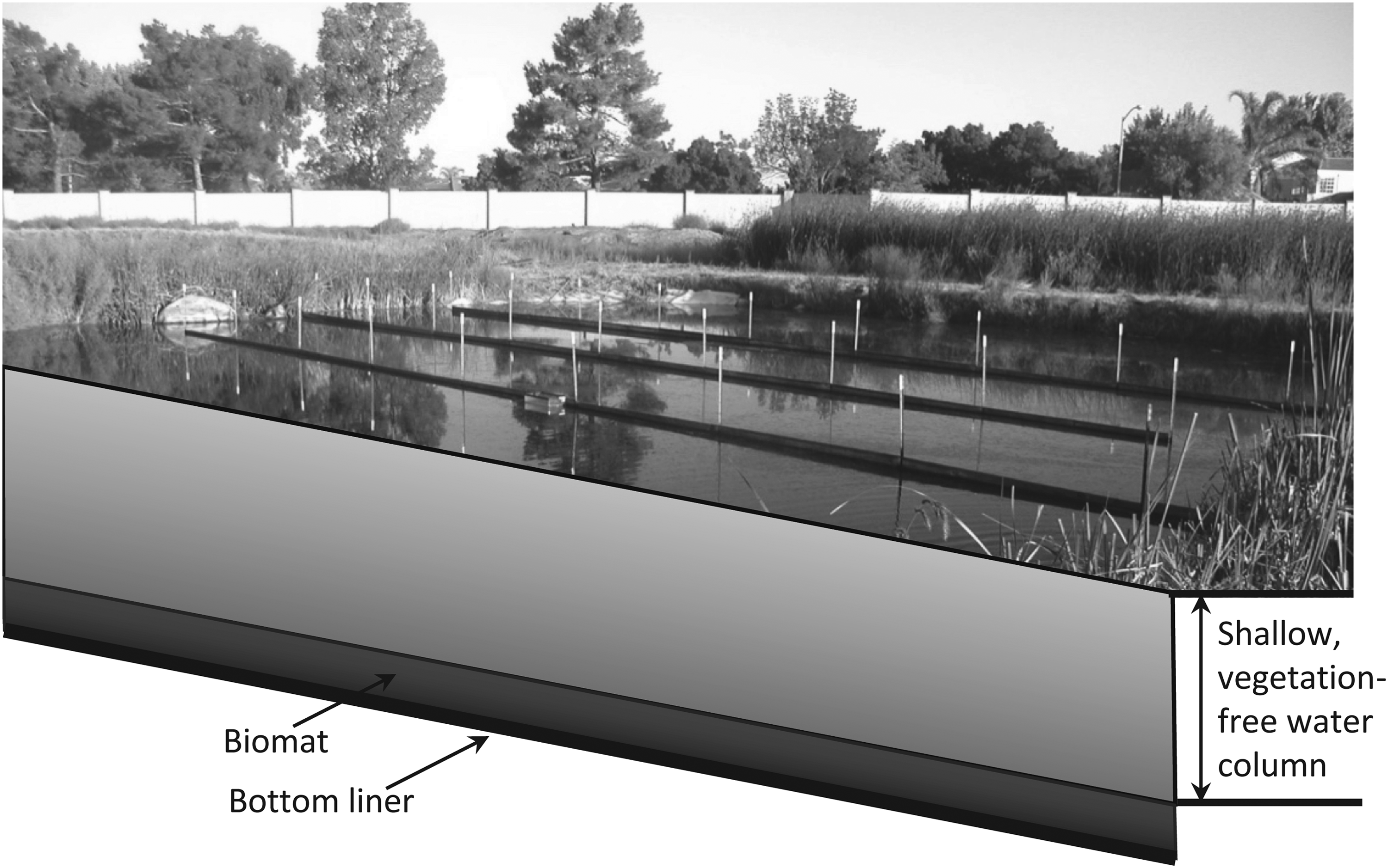
UPOW wetlands have two definitive features that influence their treatment efficiency (Fig. 1). First, UPOW wetlands have a shallow, vegetation-free water column that allows greater sunlight penetration compared with vegetated wetlands and algae-dominated ponds. To date, UPOW wetlands have been constructed with 20–30 cm water depths and a bottom liner (e.g., concrete or geotextile) to prevent the rooting of macrophytes (e.g., cattails, bulrush) that would otherwise thrive in shallow, nutrient-rich waters. Increased light penetration and the exclusion of vegetation that would shade the water surface help to promote photomediated transformation of wastewater constituents (Jasper and Sedlak, 2013; Nguyen et al., 2015; Silverman et al., 2015). The absence of rooted plants also aids hydraulic performance by minimizing preferential water flow paths that can form through vegetated regions.
Definitive features of a unit process, open-water wetland: the bottom liner, shallow vegetation-free water column, and biomat are shown in the side profile.
Second, UPOW wetlands have a diffuse, porous, biomat layer that naturally accumulates on the bottom of these systems. The biomat is composed of a consortium of photosynthetic algae (dominated by diatoms), associated heterotrophic bacteria and algal symbionts, and detritus (Jasper et al., 2014b; Jones et al., 2017, 2018), and is involved in nitrogen removal (Jasper et al., 2014b; Jones et al., 2017, 2018), and biotransformation of trace organic contaminants (TrOCs) (Jasper et al., 2014a; Prasse et al., 2015). Photosynthetic organisms within the top layer of the biomat are responsible for the high pH and dissolved oxygen (DO) concentrations measured at the surface of the biomat and in the overlying water column. Within the biomat, however, biological activity results in the rapid consumption of DO, and the occurrence of a diurnal redox gradient that ranges from supersaturated with oxygen during the daytime at the top 1 cm of the biomat, to nitrate and sulfate-reducing in the center of the biomat, and methanogenic at the bottom of the biomat (Jasper et al., 2014a). The redox gradient allows for the growth and survival of a diverse community of microorganisms that are involved in a range of transformation pathways (Jasper et al., 2014a; Jones et al., 2017), including denitrification and anammox (Jasper et al., 2014b; Jones et al., 2017, 2018). Biomat-associated microorganisms also transform a larger range of TrOCs than the less diverse microbial community in conventional wastewater treatment systems (Jasper et al., 2014a).
Municipal wastewater is an important source of nitrate (Carey and Migliaccio, 2009), numerous TrOCs (e.g., pharmaceuticals and personal care products, disinfection byproducts, steroid hormones) (Snyder et al., 2003; Ternes et al., 2004), and microbial contaminants in the aquatic environment. Given their relatively low cost and the diversity of removal processes inherent in shallow UPOW wetlands, these systems can provide a valuable option for removal of contaminants from wastewater treatment plant effluent, and act as a barrier between wastewater treatment plants and receiving waters (Jasper et al., 2013). Recent research has provided insight into the dominant treatment mechanisms and performance of laboratory-, pilot-, and demonstration-scale UPOW wetlands (Jasper and Sedlak, 2013; Jasper et al., 2014a, 2014b; Nguyen et al., 2015; Prasse et al., 2015; Silverman et al., 2015; Bear et al., 2017; Jones et al., 2017); this work has resulted in the development of numerical models that describe the decay rates of nitrate, representative TrOCs, and microbial contaminants in UPOW wetlands as a function of water quality, and environmental and contaminant characteristics. The ultimate goal of this modeling effort was to produce equations that could be used by wetland planners to design UPOW wetlands that meet water quality objectives. These equations have been validated in a pilot-scale UPOW wetland in Discovery Bay, CA (Jasper et al., 2014a, 2014b; Nguyen et al., 2015; Silverman et al., 2015) and demonstration-scale UPOW wetlands located within the Prado Treatment Wetlands in Riverside County, CA (Bear et al., 2017).
However, given the complexity of photodegradation processes and daily fluctuation of sunlight irradiance, the numerical models for predicting the removal rate constants for TrOCs and microbial contaminants are too complex to facilitate a practical design approach. Therefore, the goal of this article was to calculate and present photodegradation rates to predict the removal of TrOCs (atenolol, propranolol, sulfamethoxazole, and carbamazepine) and microbial indicator organisms (Escherichia coli and MS2) in a manner that allows for a simplified design process for UPOW wetlands.
A summary of all model equations and inputs required to predict nitrate, TrOC, and microbial contaminant removal rates in UPOW wetlands is presented. Photodegradation rate constants were determined for a range of conditions (i.e., time of year, pH, latitude, and dissolved organic carbon concentration ([DOC])), and are presented in a series of figures that can be used by practitioners when designing UPOW wetlands. We illustrate the use of these figures for UPOW wetland design with a representative example of the design process. A spreadsheet containing sample calculations is included in the Supplementary Data, which can be used to calculate rate constants for conditions not represented in the design figures.
Materials and Methods
Overall decay rate equations for TrOC and microorganisms
TrOCs in UPOW wetlands are transformed through photolysis, biotransformation, or a combination of the two (Jasper and Sedlak, 2013; Jasper et al., 2014a; Prasse et al., 2015; Bear et al., 2017); sorption was not found to be an important removal mechanism when not coupled with biotransformation (Jasper et al., 2014a). Photolysis can occur through direct and indirect processes (Schwarzenbach et al., 2003). Direct photolysis is caused when compounds absorb photons of light directly, resulting in cleavage of chemical bonds. Indirect photolysis differs from direct photolysis in that photons are first absorbed by sensitizer molecules [such as dissolved organic matter (DOM)], which then produce photochemically produced reactive intermediates (PPRI) that can oxidize target compounds. Important PPRI include hydroxyl radical (\documentclass{aastex}\usepackage{amsbsy}\usepackage{amsfonts}\usepackage{amssymb}\usepackage{bm}\usepackage{mathrsfs}\usepackage{pifont}\usepackage{stmaryrd}\usepackage{textcomp}\usepackage{portland, xspace}\usepackage{amsmath, amsxtra}\usepackage{upgreek}\pagestyle{empty}\DeclareMathSizes{10}{9}{7}{6}\begin{document}
$$\bullet { \rm{OH}}$$
\end{document}), carbonate radical (\documentclass{aastex}\usepackage{amsbsy}\usepackage{amsfonts}\usepackage{amssymb}\usepackage{bm}\usepackage{mathrsfs}\usepackage{pifont}\usepackage{stmaryrd}\usepackage{textcomp}\usepackage{portland, xspace}\usepackage{amsmath, amsxtra}\usepackage{upgreek}\pagestyle{empty}\DeclareMathSizes{10}{9}{7}{6}\begin{document}
$$\bullet { \rm{CO}}_3^{ - }$$
\end{document}), singlet oxygen (1O2), and excited triplet state dissolved organic matter (3DOM*) (Hoigne et al., 1988; Zepp, 1988; Blough and Zepp, 1995; Jasper and Sedlak, 2013).
TrOC decay rates were estimated based on the numeric models created by Jasper and Sedlak (2013) and Jasper et al. (2014a), which have already been validated at the Discovery Bay (Jasper et al., 2014a) and Prado (Bear et al., 2017) UPOW wetlands. Given that TrOC removal in open-water wetlands occurs through photolysis and biotransformation, the total transformation rate of a particular contaminant i (\documentclass{aastex}\usepackage{amsbsy}\usepackage{amsfonts}\usepackage{amssymb}\usepackage{bm}\usepackage{mathrsfs}\usepackage{pifont}\usepackage{stmaryrd}\usepackage{textcomp}\usepackage{portland, xspace}\usepackage{amsmath, amsxtra}\usepackage{upgreek}\pagestyle{empty}\DeclareMathSizes{10}{9}{7}{6}\begin{document}
$$k_{{ \rm{TrOC}}}^i$$
\end{document}; day−1) was modeled as the sum of the photolysis rate (\documentclass{aastex}\usepackage{amsbsy}\usepackage{amsfonts}\usepackage{amssymb}\usepackage{bm}\usepackage{mathrsfs}\usepackage{pifont}\usepackage{stmaryrd}\usepackage{textcomp}\usepackage{portland, xspace}\usepackage{amsmath, amsxtra}\usepackage{upgreek}\pagestyle{empty}\DeclareMathSizes{10}{9}{7}{6}\begin{document}
$$k_{{ \rm{photo}}}^i$$
\end{document}; day−1) and the biotransformation rate (\documentclass{aastex}\usepackage{amsbsy}\usepackage{amsfonts}\usepackage{amssymb}\usepackage{bm}\usepackage{mathrsfs}\usepackage{pifont}\usepackage{stmaryrd}\usepackage{textcomp}\usepackage{portland, xspace}\usepackage{amsmath, amsxtra}\usepackage{upgreek}\pagestyle{empty}\DeclareMathSizes{10}{9}{7}{6}\begin{document}
$$k_{{ \rm{bio}}}^i$$
\end{document}; day−1).
\documentclass{aastex}\usepackage{amsbsy}\usepackage{amsfonts}\usepackage{amssymb}\usepackage{bm}\usepackage{mathrsfs}\usepackage{pifont}\usepackage{stmaryrd}\usepackage{textcomp}\usepackage{portland, xspace}\usepackage{amsmath, amsxtra}\usepackage{upgreek}\pagestyle{empty}\DeclareMathSizes{10}{9}{7}{6}\begin{document}
\begin{align*}
k_{{ \rm{TrOC}}}^i = k_{{ \rm{photo}}}^i + k_{{ \rm{bio}}}^i \tag{1}
\end{align*}
\end{document}
Equations used to estimate \documentclass{aastex}\usepackage{amsbsy}\usepackage{amsfonts}\usepackage{amssymb}\usepackage{bm}\usepackage{mathrsfs}\usepackage{pifont}\usepackage{stmaryrd}\usepackage{textcomp}\usepackage{portland, xspace}\usepackage{amsmath, amsxtra}\usepackage{upgreek}\pagestyle{empty}\DeclareMathSizes{10}{9}{7}{6}\begin{document}
$$k_{{ \rm{photo}}}^i$$
\end{document} are described in a subsequent section, and sample calculations are provided in a spreadsheet included in the Supplementary Data. Biotransformation rates vary seasonally due to reduced microbial activity at lower temperatures. Consequently, \documentclass{aastex}\usepackage{amsbsy}\usepackage{amsfonts}\usepackage{amssymb}\usepackage{bm}\usepackage{mathrsfs}\usepackage{pifont}\usepackage{stmaryrd}\usepackage{textcomp}\usepackage{portland, xspace}\usepackage{amsmath, amsxtra}\usepackage{upgreek}\pagestyle{empty}\DeclareMathSizes{10}{9}{7}{6}\begin{document}
$$k_{{ \rm{bio}}}^i$$
\end{document} (day−1) was modeled as a function of air temperature (T; Kelvin) using a modified Arrhenius equation (Jasper et al., 2014a):
\documentclass{aastex}\usepackage{amsbsy}\usepackage{amsfonts}\usepackage{amssymb}\usepackage{bm}\usepackage{mathrsfs}\usepackage{pifont}\usepackage{stmaryrd}\usepackage{textcomp}\usepackage{portland, xspace}\usepackage{amsmath, amsxtra}\usepackage{upgreek}\pagestyle{empty}\DeclareMathSizes{10}{9}{7}{6}\begin{document}
\begin{align*}
k_{{ \rm{bio}}}^i = k_{{ \rm{bio , ref}}}^i{ \rm{ \;}}{{ \rm{e}}^{ - { \rm{ {\upkappa} }} \left( {{T_{{ \rm{ref}}}} - T} \right) }} \tag{2}
\end{align*}
\end{document}
where \documentclass{aastex}\usepackage{amsbsy}\usepackage{amsfonts}\usepackage{amssymb}\usepackage{bm}\usepackage{mathrsfs}\usepackage{pifont}\usepackage{stmaryrd}\usepackage{textcomp}\usepackage{portland, xspace}\usepackage{amsmath, amsxtra}\usepackage{upgreek}\pagestyle{empty}\DeclareMathSizes{10}{9}{7}{6}\begin{document}
$$k_{{ \rm{bio , ref}}}^i$$
\end{document} (day−1; values provided in Supplementary Table S2) is the biotransformation rate at reference temperature Tref (300.15 K = 27°C), and κ (K−1) is the temperature coefficient. Typical κ values for TrOC range between 0.03 and 0.09 K−1; Jasper et al. (2014a) used an average value of 0.06 K−1. A limitation of the biotransformation model is that the effect of the biomat thickness on TrOC biotransformation rates is not fully understood, and is therefore not reflected in the biotransformation rate equation (i.e., biotransformation rates are assumed to stay constant for different biomat thicknesses). However, variations in biomat thickness can affect the redox gradient within the biomat, which could thereby affect the microorganism community composition and, subsequently, biotransformation rates.
Sunlight inactivation is an important mode of disinfection of bacteria and viruses in UPOW wetlands, and has been found to be as or more important than sedimentation or other dark removal processes (Davies-Colley, 2005). Sunlight inactivation of waterborne bacteria and viruses occurs through two main mechanisms: endogenous photoinactivation and exogenous photoinactivation (Davies-Colley et al., 1999, 2000). Endogenous photoinactivation occurs through damage to biomolecules within the microorganism (i.e., nucleic acids and amino acids) when sunlight is absorbed by the microorganism itself (Cunningham et al., 1985; Jagger, 1985). The exogenous photoinactivation mechanism is similar to indirect photolysis of TrOC in that damage is caused by PPRI produced by sensitizers that reside in the water column outside the cell or virion. 1O2 is often the most important PPRI for exogenous inactivation of bacteria (Kadir and Nelson, 2014) and viruses (Kohn and Nelson, 2007; Mattle et al., 2015).
Susceptibilities to each sunlight inactivation mechanism differ among microorganisms. In general, viruses have slower photoinactivation rates than bacteria (Sinton et al., 1999, 2002), and within the viruses, bacteriophage MS2 has a slower endogenous photoinactivation rate than many other human viruses and bacteriophage (Love et al., 2010; Romero et al., 2011; Silverman et al., 2013; Mattle et al., 2015). Therefore, while the general framework of the bacteria and virus inactivation rate equations are the same across microorganisms, they contain species-specific parameters. Sunlight inactivation rates were estimated based on the numeric models created by Fisher et al. (2011), Silverman et al. (2015), Nguyen et al. (2015), and Silverman and Nelson (2016), and were previously validated at the Discovery Bay UPOW wetland. The total sunlight inactivation rate of a bacterium or virus i (\documentclass{aastex}\usepackage{amsbsy}\usepackage{amsfonts}\usepackage{amssymb}\usepackage{bm}\usepackage{mathrsfs}\usepackage{pifont}\usepackage{stmaryrd}\usepackage{textcomp}\usepackage{portland, xspace}\usepackage{amsmath, amsxtra}\usepackage{upgreek}\pagestyle{empty}\DeclareMathSizes{10}{9}{7}{6}\begin{document}
$$k_{{ \rm{microbial}}}^i$$
\end{document}; day−1) was estimated as the sum of the first-order endogenous (\documentclass{aastex}\usepackage{amsbsy}\usepackage{amsfonts}\usepackage{amssymb}\usepackage{bm}\usepackage{mathrsfs}\usepackage{pifont}\usepackage{stmaryrd}\usepackage{textcomp}\usepackage{portland, xspace}\usepackage{amsmath, amsxtra}\usepackage{upgreek}\pagestyle{empty}\DeclareMathSizes{10}{9}{7}{6}\begin{document}
$$k_{{ \rm{endo}}}^i$$
\end{document}; day−1), exogenous (\documentclass{aastex}\usepackage{amsbsy}\usepackage{amsfonts}\usepackage{amssymb}\usepackage{bm}\usepackage{mathrsfs}\usepackage{pifont}\usepackage{stmaryrd}\usepackage{textcomp}\usepackage{portland, xspace}\usepackage{amsmath, amsxtra}\usepackage{upgreek}\pagestyle{empty}\DeclareMathSizes{10}{9}{7}{6}\begin{document}
$$k_{{ \rm{exo}}}^i$$
\end{document}; day−1), and dark (\documentclass{aastex}\usepackage{amsbsy}\usepackage{amsfonts}\usepackage{amssymb}\usepackage{bm}\usepackage{mathrsfs}\usepackage{pifont}\usepackage{stmaryrd}\usepackage{textcomp}\usepackage{portland, xspace}\usepackage{amsmath, amsxtra}\usepackage{upgreek}\pagestyle{empty}\DeclareMathSizes{10}{9}{7}{6}\begin{document}
$$k_{{ \rm{dark}}}^i$$
\end{document}; day−1) inactivation rates. All inactivation rates were calculated assuming a well-mixed water column.
\documentclass{aastex}\usepackage{amsbsy}\usepackage{amsfonts}\usepackage{amssymb}\usepackage{bm}\usepackage{mathrsfs}\usepackage{pifont}\usepackage{stmaryrd}\usepackage{textcomp}\usepackage{portland, xspace}\usepackage{amsmath, amsxtra}\usepackage{upgreek}\pagestyle{empty}\DeclareMathSizes{10}{9}{7}{6}\begin{document}
\begin{align*}
k_{{ \rm{microbial}}}^i = k_{{ \rm{endo}}}^i + k_{{ \rm{exo}}}^i + k_{{ \rm{dark}}}^i \tag{3}
\end{align*}
\end{document}
Equations used to estimate \documentclass{aastex}\usepackage{amsbsy}\usepackage{amsfonts}\usepackage{amssymb}\usepackage{bm}\usepackage{mathrsfs}\usepackage{pifont}\usepackage{stmaryrd}\usepackage{textcomp}\usepackage{portland, xspace}\usepackage{amsmath, amsxtra}\usepackage{upgreek}\pagestyle{empty}\DeclareMathSizes{10}{9}{7}{6}\begin{document}
$$k_{{ \rm{endo}}}^i$$
\end{document} and \documentclass{aastex}\usepackage{amsbsy}\usepackage{amsfonts}\usepackage{amssymb}\usepackage{bm}\usepackage{mathrsfs}\usepackage{pifont}\usepackage{stmaryrd}\usepackage{textcomp}\usepackage{portland, xspace}\usepackage{amsmath, amsxtra}\usepackage{upgreek}\pagestyle{empty}\DeclareMathSizes{10}{9}{7}{6}\begin{document}
$$k_{{ \rm{exo}}}^i$$
\end{document} are described in a subsequent section, and sample calculations are provided in a spreadsheet in the Supplementary Data. Based on studies conducted in the laboratory using water from the Discovery Bay UPOW wetland, E. coli had an average \documentclass{aastex}\usepackage{amsbsy}\usepackage{amsfonts}\usepackage{amssymb}\usepackage{bm}\usepackage{mathrsfs}\usepackage{pifont}\usepackage{stmaryrd}\usepackage{textcomp}\usepackage{portland, xspace}\usepackage{amsmath, amsxtra}\usepackage{upgreek}\pagestyle{empty}\DeclareMathSizes{10}{9}{7}{6}\begin{document}
$$k_{{ \rm{dark}}}^{E. \;coli}$$
\end{document} of 0.86 day−1 (Nguyen et al., 2015), whereas MS2 was not significantly inactivated by dark mechanisms (i.e., \documentclass{aastex}\usepackage{amsbsy}\usepackage{amsfonts}\usepackage{amssymb}\usepackage{bm}\usepackage{mathrsfs}\usepackage{pifont}\usepackage{stmaryrd}\usepackage{textcomp}\usepackage{portland, xspace}\usepackage{amsmath, amsxtra}\usepackage{upgreek}\pagestyle{empty}\DeclareMathSizes{10}{9}{7}{6}\begin{document}
$$k_{{ \rm{dark}}}^{{ \rm{MS}}2}$$
\end{document} = 0) (Kohn and Nelson, 2007; Love et al., 2010; Silverman et al., 2013, 2015).
Choice of indicator compounds and microorganisms
There are hundreds of potential contaminants of concern in municipal wastewater effluent—it is not possible to monitor or model decay of every one. As an alternative, indicator compounds can provide insight into the behavior of a suite of contaminants (Dickenson et al., 2009, 2011). Therefore, four compounds that are regularly detected in municipal wastewater were selected as indicator compounds to represent a range of TrOC transformation behaviors, based on the findings of Jasper and Sedlak (2013) and Jasper et al. (2014a) (Fig. 2):
Atenolol (beta blocker)—transformation dominated by biotransformation, with a small contribution from photolysis (Jasper et al., 2014a).
Propranolol (beta blocker)—transformation dominated by indirect photolysis, with a small contribution from biological transformation (Jasper et al., 2014a). The PPRI most involved in photolysis was 3DOM* (Jasper and Sedlak, 2013).
Sulfamethoxazole (antibiotic)—transformation also dominated by indirect photolysis, but with a slower transformation rate than propranolol. Sulfamethoxazole photolysis was mostly attributed to reaction with \documentclass{aastex}\usepackage{amsbsy}\usepackage{amsfonts}\usepackage{amssymb}\usepackage{bm}\usepackage{mathrsfs}\usepackage{pifont}\usepackage{stmaryrd}\usepackage{textcomp}\usepackage{portland, xspace}\usepackage{amsmath, amsxtra}\usepackage{upgreek}\pagestyle{empty}\DeclareMathSizes{10}{9}{7}{6}\begin{document}
$$\bullet { \rm{CO}}_3^{ - { \rm{ \;}}}$$
\end{document} (Jasper and Sedlak, 2013).
Carbamazepine (anticonvulsant)—recalcitrant, with slow photolysis and biological transformation rates in open-water wetlands. Decay was attributed to indirect photolysis, mainly through reaction with •OH (Jasper and Sedlak, 2013).
Trace organic contaminant removal rates attributed to each removal mechanism (i.e., biotransformation, direct photolysis, indirect photolysis). Transformation rates were estimated with pH = 8; [DOC] = 7.5 mg-C L−1; a 30-cm-deep, well-mixed water column; irradiance estimated for 35°N latitude in June; and air temperature = 22°C. [DOC], dissolved organic carbon concentration.
Similarly, wastewater can contain a broad range of microbial contaminants, requiring the use of indicator microorganisms to represent disinfection behavior. The fecal indicator bacteria E. coli was chosen to represent bacteria inactivation, and bacteriophage MS2 was used to model virus inactivation. E. coli is susceptible to endogenous, but not exogenous, photoinactivation (Nguyen et al., 2015). MS2 is susceptible to both endogenous and exogenous photoinactivation, although it is more resistant to the endogenous mechanism than E. coli (Silverman et al., 2015).
Inputs to photolysis and photoinactivation models: environmental and water quality conditions
Subsequent sections outline the equations used to model photolysis and photoinactivation rates in UPOW wetlands, which have a strong dependence on environmental and water quality conditions. These factors include (1) the solar intensity incident on the water surface (which depends on latitude, season, cloud cover, and time of day); (2) [DOC] (which influences light attenuation in the water column and formation of PPRI); and, (3) pH, which affects formation rates of PPRI and reaction rates between TrOC and PPRI. Photolysis and photoinactivation rates are not expected to depend on temperature within the range observed in UPOW wetlands.
Photolysis and photoinactivation rates were determined for well-mixed water columns with depths of 20, 30, and 40 cm; a 5-cm-thick biomat was assumed for all depths. The following representative values were used as inputs for environmental and water quality variables:
Time of year—photolysis and photoinactivation rates were determined for three representative dates: December 21, March (or September) 21, and June 21; these dates correspond to the winter solstice, the March (and September) equinoxes, and the summer solstice for the northern hemisphere.
Latitude—photolysis and photoinactivation rates were determined for the following latitudes: equator (00°), 10°N, 20°N, 30°N, 40°N, and 50°N. Photolysis and photoinactivation rates determined at these latitudes can be applied to the southern hemisphere if values for December and June are switched.
[DOC]—[DOC] affects both light transmission through the water column (therefore direct photolysis) and formation of PPRI (therefore indirect photolysis). Waters with [DOC] in the range of 5 to 20 mg-C L−1 were modeled.
pH—two pH values were input to photolysis equations: pH 8 and pH 10, which span the pH range measured in UPOW wetlands.
Irradiance spectra used to estimate photolysis and photoinactivation rates were predicted using the Simple Model of the Atmospheric Radiative Transfer of Sunshine (SMARTS) (Gueymard, 1995, 2001). SMARTS is a computational model hosted by NREL (www.nrel.gov/rredc/smarts/) that can estimate sunlight irradiance at any location, day of year, time, or elevation. Therefore, SMARTS can account for diurnal and seasonal changes in irradiance. However, an important limitation of SMARTS is that the model assumes clear-sky conditions and does not account for variations in atmospheric conditions or cloud cover that could decrease irradiance. The impact of cloud cover on irradiance spectra depends on the extent of coverage, cloud thickness, and the type of cloud (Bartlett et al., 1998). Therefore, the effect of cloud cover on photolysis rates is difficult to generalize and is the subject of ongoing work. Inputs to SMARTS are provided in the Supplementary Data (Supplementary Table S1) and modeled irradiance spectra are presented in Supplementary Fig. S1 of the Supplementary Data.
Determination of TrOC kiphoto
The framework and equations for calculating TrOC photolysis are summarized in this section and come from Jasper and Sedlak (2013). As discussed above, photolysis can occur through direct and indirect processes (Schwarzenbach et al., 2003). Depending on the compound, both photolysis processes can be important; therefore, \documentclass{aastex}\usepackage{amsbsy}\usepackage{amsfonts}\usepackage{amssymb}\usepackage{bm}\usepackage{mathrsfs}\usepackage{pifont}\usepackage{stmaryrd}\usepackage{textcomp}\usepackage{portland, xspace}\usepackage{amsmath, amsxtra}\usepackage{upgreek}\pagestyle{empty}\DeclareMathSizes{10}{9}{7}{6}\begin{document}
$$k_{{ \rm{photo}}}^i$$
\end{document} (day−1) of a particular compound i was modeled as the sum of the two processes, using the following equation (Jasper and Sedlak, 2013):
\documentclass{aastex}\usepackage{amsbsy}\usepackage{amsfonts}\usepackage{amssymb}\usepackage{bm}\usepackage{mathrsfs}\usepackage{pifont}\usepackage{stmaryrd}\usepackage{textcomp}\usepackage{portland, xspace}\usepackage{amsmath, amsxtra}\usepackage{upgreek}\pagestyle{empty}\DeclareMathSizes{10}{9}{7}{6}\begin{document}
\begin{align*}
k_ { { \rm { photo } } } ^i = \frac { { \left( { z - { d_ { { \rm { biomat } } } } } \right) } } { z } \cdot \left( { k_ { { \rm { direct } } } ^i + k_ { { \rm { indirect } } } ^i } \right) \tag { 4 }
\end{align*}
\end{document}
\documentclass{aastex}\usepackage{amsbsy}\usepackage{amsfonts}\usepackage{amssymb}\usepackage{bm}\usepackage{mathrsfs}\usepackage{pifont}\usepackage{stmaryrd}\usepackage{textcomp}\usepackage{portland, xspace}\usepackage{amsmath, amsxtra}\usepackage{upgreek}\pagestyle{empty}\DeclareMathSizes{10}{9}{7}{6}\begin{document}
$$k_{{ \rm{direct}}}^i$$
\end{document} [day−1; Eq. (5)] is the first-order direct photolysis rate constant, \documentclass{aastex}\usepackage{amsbsy}\usepackage{amsfonts}\usepackage{amssymb}\usepackage{bm}\usepackage{mathrsfs}\usepackage{pifont}\usepackage{stmaryrd}\usepackage{textcomp}\usepackage{portland, xspace}\usepackage{amsmath, amsxtra}\usepackage{upgreek}\pagestyle{empty}\DeclareMathSizes{10}{9}{7}{6}\begin{document}
$$k_{{ \rm{indirect}}}^i$$
\end{document} [day−1; Eq. (10)] is the first-order indirect photolysis rate constant, z (cm) is the total depth of the water column, and dbiomat (cm) is the thickness of the biomat. Given that sunlight is required for photolysis to occur, and assuming that the water column is well mixed across the depth (including the volume occupied by the biomat), the photolysis rate was corrected for time the water spends shaded within the biomat by using the term \documentclass{aastex}\usepackage{amsbsy}\usepackage{amsfonts}\usepackage{amssymb}\usepackage{bm}\usepackage{mathrsfs}\usepackage{pifont}\usepackage{stmaryrd}\usepackage{textcomp}\usepackage{portland, xspace}\usepackage{amsmath, amsxtra}\usepackage{upgreek}\pagestyle{empty}\DeclareMathSizes{10}{9}{7}{6}\begin{document}
$${{ \left( {z - {d_{{ \rm{biomat}}}}} \right) } / z} $$
\end{document} (Jasper et al., 2014a; Silverman et al., 2015).
\documentclass{aastex}\usepackage{amsbsy}\usepackage{amsfonts}\usepackage{amssymb}\usepackage{bm}\usepackage{mathrsfs}\usepackage{pifont}\usepackage{stmaryrd}\usepackage{textcomp}\usepackage{portland, xspace}\usepackage{amsmath, amsxtra}\usepackage{upgreek}\pagestyle{empty}\DeclareMathSizes{10}{9}{7}{6}\begin{document}
$$k_{{ \rm{direct}}}^i$$
\end{document} was estimated using Equation (5) with the following inputs: the quantum yields specific to compound i (\documentclass{aastex}\usepackage{amsbsy}\usepackage{amsfonts}\usepackage{amssymb}\usepackage{bm}\usepackage{mathrsfs}\usepackage{pifont}\usepackage{stmaryrd}\usepackage{textcomp}\usepackage{portland, xspace}\usepackage{amsmath, amsxtra}\usepackage{upgreek}\pagestyle{empty}\DeclareMathSizes{10}{9}{7}{6}\begin{document}
$${ \rm{ \Phi }}_{{ \rm{prot}}}^i$$
\end{document} and \documentclass{aastex}\usepackage{amsbsy}\usepackage{amsfonts}\usepackage{amssymb}\usepackage{bm}\usepackage{mathrsfs}\usepackage{pifont}\usepackage{stmaryrd}\usepackage{textcomp}\usepackage{portland, xspace}\usepackage{amsmath, amsxtra}\usepackage{upgreek}\pagestyle{empty}\DeclareMathSizes{10}{9}{7}{6}\begin{document}
$${ \rm{ \Phi }}_{{ \rm{unprot}}}^i$$
\end{document}; mol molecules transformed/mol photons absorbed; Supplementary Table S4), the 24 h-averaged photon fluence rate incident on the water surface [Z24h avg(λ); Einstein (cm2 day)−1Eq. (7)], a light screening factor that corrects the incident light spectrum for attenuation in a well-mixed water column [S(λ, z); Eq. (8)] (Schwarzenbach et al., 2003), and the molar absorption coefficient spectrum (ɛi(λ); M−1 cm−1; Supplementary Table S3). The term \documentclass{aastex}\usepackage{amsbsy}\usepackage{amsfonts}\usepackage{amssymb}\usepackage{bm}\usepackage{mathrsfs}\usepackage{pifont}\usepackage{stmaryrd}\usepackage{textcomp}\usepackage{portland, xspace}\usepackage{amsmath, amsxtra}\usepackage{upgreek}\pagestyle{empty}\DeclareMathSizes{10}{9}{7}{6}\begin{document}
$${ \rm{ \alpha }}_0^i$$
\end{document} describes the acid–base speciation of compound i, given that the quantum yield can differ depending on whether the compound is in its protonated (\documentclass{aastex}\usepackage{amsbsy}\usepackage{amsfonts}\usepackage{amssymb}\usepackage{bm}\usepackage{mathrsfs}\usepackage{pifont}\usepackage{stmaryrd}\usepackage{textcomp}\usepackage{portland, xspace}\usepackage{amsmath, amsxtra}\usepackage{upgreek}\pagestyle{empty}\DeclareMathSizes{10}{9}{7}{6}\begin{document}
$${ \rm{ \Phi }}_{{ \rm{prot}}}^i$$
\end{document}) or unprotonated (\documentclass{aastex}\usepackage{amsbsy}\usepackage{amsfonts}\usepackage{amssymb}\usepackage{bm}\usepackage{mathrsfs}\usepackage{pifont}\usepackage{stmaryrd}\usepackage{textcomp}\usepackage{portland, xspace}\usepackage{amsmath, amsxtra}\usepackage{upgreek}\pagestyle{empty}\DeclareMathSizes{10}{9}{7}{6}\begin{document}
$${ \rm{ \Phi }}_{{ \rm{unprot}}}^i$$
\end{document}) form. \documentclass{aastex}\usepackage{amsbsy}\usepackage{amsfonts}\usepackage{amssymb}\usepackage{bm}\usepackage{mathrsfs}\usepackage{pifont}\usepackage{stmaryrd}\usepackage{textcomp}\usepackage{portland, xspace}\usepackage{amsmath, amsxtra}\usepackage{upgreek}\pagestyle{empty}\DeclareMathSizes{10}{9}{7}{6}\begin{document}
$${ \rm{ \alpha }}_0^i$$
\end{document} is computed in Equation (6), and pKai are provided in Supplementary Table S4.
Z24h avg(λ) was calculated from the 24-h averaged global horizontal irradiance incident on the water surface (E24h avg(λ); W m−2) using Equation (7), where h is Planck's constant (h = 6.626 × 10⁻³⁴ J·s), c is the speed of light (c = 3.0 × 10⁸ m s−1), λ is the wavelength (nm), and u is a unit conversion factor (u = 1.435 × 10⁻³² Einstein s m3 (photon day nm cm2)−1. E24h avg(λ) was estimated using SMARTS (Gueymard, 1995, 2001). Global horizontal irradiance spectra were predicted for each hour of the 21st day of the month and averaged over 24 h to calculate the daily average.
\documentclass{aastex}\usepackage{amsbsy}\usepackage{amsfonts}\usepackage{amssymb}\usepackage{bm}\usepackage{mathrsfs}\usepackage{pifont}\usepackage{stmaryrd}\usepackage{textcomp}\usepackage{portland, xspace}\usepackage{amsmath, amsxtra}\usepackage{upgreek}\pagestyle{empty}\DeclareMathSizes{10}{9}{7}{6}\begin{document}
\begin{align*}
{ Z_ { 24 { \rm { h \;avg } } } } \left( { \rm { \lambda } } \right) = \left( { { \frac { { \rm { \lambda } } \cdot u } { h \cdot c } } } \right) { E_ { 24 { \rm { h \;avg } } } } \left( { \rm { \lambda } } \right) \tag { 7 }
\end{align*}
\end{document}
The light screening factor, S(λ, z), is wavelength dependent and was calculated for a well-mixed water column using Equation (8) (Schwarzenbach et al., 2003); inputs are the depth of the light-exposed water column (z − dbiomat; cm), the wavelength-specific decadic light absorption coefficient [α(λ); cm−1; Eq. (9)], and a path length correction factor (ψ) used to correct the depth for light path geometry. The value of ψ was assumed to be 1.2, which is an average path length correction factor calculated based on light refraction at the water surface (Zepp and Cline, 1977).
\documentclass{aastex}\usepackage{amsbsy}\usepackage{amsfonts}\usepackage{amssymb}\usepackage{bm}\usepackage{mathrsfs}\usepackage{pifont}\usepackage{stmaryrd}\usepackage{textcomp}\usepackage{portland, xspace}\usepackage{amsmath, amsxtra}\usepackage{upgreek}\pagestyle{empty}\DeclareMathSizes{10}{9}{7}{6}\begin{document}
\begin{align*}
S \left( { { \rm { \lambda } } , { \rm { \;z } } } \right) = \left( { { \frac { 1 - { { 10 } ^ { - { \rm { { \uppsi } } } \cdot { \rm { \alpha } } \left( { \rm { \lambda } } \right) \cdot ( z - { d_ { { \rm { biomat } } } } ) } } } { 2.303 \cdot { \rm { { \uppsi } } } \cdot { \rm { \alpha } } \left( { \rm { \lambda } } \right) \cdot ( z - { d_ { biomat } } ) } } } \right) \tag { 8 }
\end{align*}
\end{document}
α(λ) was estimated based on the [DOC] in the water ([DOC]; mg-C L−1) using Equation (9). Values for m(λ) and b(λ) (Supplementary Table S6) come from Jasper and Sedlak (2013) and were derived from absorbance data for over 15 samples collected from the Discovery Bay UPOW wetland on different days with a range of [DOC]. Equation (9) was previously used to model TrOC photolysis rates in the Discovery Bay UPOW wetland that received clarified secondary effluent, as well as the Prado UPOW wetland that received water from the effluent-dominated Santa Ana River. If photolysis rates are to be estimated in water sources with optical properties that may differ from the Discovery Bay and Prado UPOW wetlands, one could compare the measured absorption spectrum with that estimated by Equation (9) to determine whether photolysis rates predicted herein will apply in their context.
\documentclass{aastex}\usepackage{amsbsy}\usepackage{amsfonts}\usepackage{amssymb}\usepackage{bm}\usepackage{mathrsfs}\usepackage{pifont}\usepackage{stmaryrd}\usepackage{textcomp}\usepackage{portland, xspace}\usepackage{amsmath, amsxtra}\usepackage{upgreek}\pagestyle{empty}\DeclareMathSizes{10}{9}{7}{6}\begin{document}
\begin{align*}
{ \rm{ \alpha }} \left( { \rm{ \lambda }} \right) = m \left( { \rm{ \lambda }} \right) \left[ {{ \rm{DOC}}} \right] + b \left( { \rm{ \lambda }} \right) \tag{9}
\end{align*}
\end{document}
\documentclass{aastex}\usepackage{amsbsy}\usepackage{amsfonts}\usepackage{amssymb}\usepackage{bm}\usepackage{mathrsfs}\usepackage{pifont}\usepackage{stmaryrd}\usepackage{textcomp}\usepackage{portland, xspace}\usepackage{amsmath, amsxtra}\usepackage{upgreek}\pagestyle{empty}\DeclareMathSizes{10}{9}{7}{6}\begin{document}
$$k_{{ \rm{indirect}}}^i$$
\end{document} (day−1) was estimated using Equation (10), where \documentclass{aastex}\usepackage{amsbsy}\usepackage{amsfonts}\usepackage{amssymb}\usepackage{bm}\usepackage{mathrsfs}\usepackage{pifont}\usepackage{stmaryrd}\usepackage{textcomp}\usepackage{portland, xspace}\usepackage{amsmath, amsxtra}\usepackage{upgreek}\pagestyle{empty}\DeclareMathSizes{10}{9}{7}{6}\begin{document}
$$k_{ \bullet { \rm{OH}}}^i$$
\end{document}, \documentclass{aastex}\usepackage{amsbsy}\usepackage{amsfonts}\usepackage{amssymb}\usepackage{bm}\usepackage{mathrsfs}\usepackage{pifont}\usepackage{stmaryrd}\usepackage{textcomp}\usepackage{portland, xspace}\usepackage{amsmath, amsxtra}\usepackage{upgreek}\pagestyle{empty}\DeclareMathSizes{10}{9}{7}{6}\begin{document}
$$k_{ \bullet { \rm{CO}}_3^ - }^i$$
\end{document}, and \documentclass{aastex}\usepackage{amsbsy}\usepackage{amsfonts}\usepackage{amssymb}\usepackage{bm}\usepackage{mathrsfs}\usepackage{pifont}\usepackage{stmaryrd}\usepackage{textcomp}\usepackage{portland, xspace}\usepackage{amsmath, amsxtra}\usepackage{upgreek}\pagestyle{empty}\DeclareMathSizes{10}{9}{7}{6}\begin{document}
$$k_{{}_{}^1{{ \rm{O}}_2}}^i$$
\end{document} (M−1day−1) are the second-order reaction rate constants between contaminant i and \documentclass{aastex}\usepackage{amsbsy}\usepackage{amsfonts}\usepackage{amssymb}\usepackage{bm}\usepackage{mathrsfs}\usepackage{pifont}\usepackage{stmaryrd}\usepackage{textcomp}\usepackage{portland, xspace}\usepackage{amsmath, amsxtra}\usepackage{upgreek}\pagestyle{empty}\DeclareMathSizes{10}{9}{7}{6}\begin{document}
$$\bullet { \rm{OH}}$$
\end{document}, \documentclass{aastex}\usepackage{amsbsy}\usepackage{amsfonts}\usepackage{amssymb}\usepackage{bm}\usepackage{mathrsfs}\usepackage{pifont}\usepackage{stmaryrd}\usepackage{textcomp}\usepackage{portland, xspace}\usepackage{amsmath, amsxtra}\usepackage{upgreek}\pagestyle{empty}\DeclareMathSizes{10}{9}{7}{6}\begin{document}
$$\bullet { \rm{CO}}_3^{ - { \rm{ \;}}}$$
\end{document}, and 1O2, respectively; these values differ depending on whether contaminant i is in its protonated or unprotonated form (i.e., depending on the pH and pKai), and are provided in Supplementary Table S4. \documentclass{aastex}\usepackage{amsbsy}\usepackage{amsfonts}\usepackage{amssymb}\usepackage{bm}\usepackage{mathrsfs}\usepackage{pifont}\usepackage{stmaryrd}\usepackage{textcomp}\usepackage{portland, xspace}\usepackage{amsmath, amsxtra}\usepackage{upgreek}\pagestyle{empty}\DeclareMathSizes{10}{9}{7}{6}\begin{document}
$${ \left[ { \bullet { \rm{OH}}} \right] _{{ \rm{ss}}}}$$
\end{document}, \documentclass{aastex}\usepackage{amsbsy}\usepackage{amsfonts}\usepackage{amssymb}\usepackage{bm}\usepackage{mathrsfs}\usepackage{pifont}\usepackage{stmaryrd}\usepackage{textcomp}\usepackage{portland, xspace}\usepackage{amsmath, amsxtra}\usepackage{upgreek}\pagestyle{empty}\DeclareMathSizes{10}{9}{7}{6}\begin{document}
$${ \left[ { \bullet { \rm{CO}}_3^{ - { \rm{ \;}}}} \right] _{{ \rm{ss}}}}$$
\end{document}, and \documentclass{aastex}\usepackage{amsbsy}\usepackage{amsfonts}\usepackage{amssymb}\usepackage{bm}\usepackage{mathrsfs}\usepackage{pifont}\usepackage{stmaryrd}\usepackage{textcomp}\usepackage{portland, xspace}\usepackage{amsmath, amsxtra}\usepackage{upgreek}\pagestyle{empty}\DeclareMathSizes{10}{9}{7}{6}\begin{document}
$${ \left[ {{}_{}^1{{ \rm{O}}_2}} \right] _{{ \rm{ss}}}}$$
\end{document} (M) are the steady-state concentrations of each PPRI; these steady-state concentrations were estimated using Equations (11) through (17). \documentclass{aastex}\usepackage{amsbsy}\usepackage{amsfonts}\usepackage{amssymb}\usepackage{bm}\usepackage{mathrsfs}\usepackage{pifont}\usepackage{stmaryrd}\usepackage{textcomp}\usepackage{portland, xspace}\usepackage{amsmath, amsxtra}\usepackage{upgreek}\pagestyle{empty}\DeclareMathSizes{10}{9}{7}{6}\begin{document}
$$k_{{}_{}^3{ \rm{DO}}{{ \rm{M}}^{ \rm{*}}}}^i$$
\end{document} (day−1) is the pseudo first-order reaction rate constant between 3DOM* and contaminant i, and was estimated using Equation (18).
\documentclass{aastex}\usepackage{amsbsy}\usepackage{amsfonts}\usepackage{amssymb}\usepackage{bm}\usepackage{mathrsfs}\usepackage{pifont}\usepackage{stmaryrd}\usepackage{textcomp}\usepackage{portland, xspace}\usepackage{amsmath, amsxtra}\usepackage{upgreek}\pagestyle{empty}\DeclareMathSizes{10}{9}{7}{6}\begin{document}
$${ \left[ { \bullet { \rm{OH}}} \right] _{{ \rm{ss}}}}$$
\end{document} was estimated using Equation (11) (Jasper and Sedlak, 2013), which accounts for the rates of •OH formation by nitrate [\documentclass{aastex}\usepackage{amsbsy}\usepackage{amsfonts}\usepackage{amssymb}\usepackage{bm}\usepackage{mathrsfs}\usepackage{pifont}\usepackage{stmaryrd}\usepackage{textcomp}\usepackage{portland, xspace}\usepackage{amsmath, amsxtra}\usepackage{upgreek}\pagestyle{empty}\DeclareMathSizes{10}{9}{7}{6}\begin{document}
$${R_{{ \rm{form}} , \bullet { \rm{OH}} , { \rm{ \;NO}}_3^ - }}$$
\end{document}; M day−1; Eq. (14)] and DOM [\documentclass{aastex}\usepackage{amsbsy}\usepackage{amsfonts}\usepackage{amssymb}\usepackage{bm}\usepackage{mathrsfs}\usepackage{pifont}\usepackage{stmaryrd}\usepackage{textcomp}\usepackage{portland, xspace}\usepackage{amsmath, amsxtra}\usepackage{upgreek}\pagestyle{empty}\DeclareMathSizes{10}{9}{7}{6}\begin{document}
$${R_{{ \rm{form}} , \bullet { \rm{OH}} , { \rm{ \;DOM}}}}$$
\end{document}; M day−1; Eq. (15)], as well as the second-order rates of •OH scavenging by carbonate species (\documentclass{aastex}\usepackage{amsbsy}\usepackage{amsfonts}\usepackage{amssymb}\usepackage{bm}\usepackage{mathrsfs}\usepackage{pifont}\usepackage{stmaryrd}\usepackage{textcomp}\usepackage{portland, xspace}\usepackage{amsmath, amsxtra}\usepackage{upgreek}\pagestyle{empty}\DeclareMathSizes{10}{9}{7}{6}\begin{document}
$${k_{ \bullet { \rm{OH}} , { \rm{HCO}}_3^ - }}$$
\end{document} and \documentclass{aastex}\usepackage{amsbsy}\usepackage{amsfonts}\usepackage{amssymb}\usepackage{bm}\usepackage{mathrsfs}\usepackage{pifont}\usepackage{stmaryrd}\usepackage{textcomp}\usepackage{portland, xspace}\usepackage{amsmath, amsxtra}\usepackage{upgreek}\pagestyle{empty}\DeclareMathSizes{10}{9}{7}{6}\begin{document}
$${k_{ \bullet { \rm{OH}} , { \rm{CO}}_3^{2 - }}}$$
\end{document}; M−1 day−1; Supplementary Table S5) and DOM (\documentclass{aastex}\usepackage{amsbsy}\usepackage{amsfonts}\usepackage{amssymb}\usepackage{bm}\usepackage{mathrsfs}\usepackage{pifont}\usepackage{stmaryrd}\usepackage{textcomp}\usepackage{portland, xspace}\usepackage{amsmath, amsxtra}\usepackage{upgreek}\pagestyle{empty}\DeclareMathSizes{10}{9}{7}{6}\begin{document}
$${k_{ \bullet { \rm{OH}} , { \rm{DOM}}}}$$
\end{document}; (mg L−1-C)−1 day−1; Supplementary Table S5).
DOM was approximated as [DOC]. The concentrations of bicarbonate ([\documentclass{aastex}\usepackage{amsbsy}\usepackage{amsfonts}\usepackage{amssymb}\usepackage{bm}\usepackage{mathrsfs}\usepackage{pifont}\usepackage{stmaryrd}\usepackage{textcomp}\usepackage{portland, xspace}\usepackage{amsmath, amsxtra}\usepackage{upgreek}\pagestyle{empty}\DeclareMathSizes{10}{9}{7}{6}\begin{document}
$$ {{ \rm{HCO}}_3^ - }$$
\end{document}]) and carbonate ([\documentclass{aastex}\usepackage{amsbsy}\usepackage{amsfonts}\usepackage{amssymb}\usepackage{bm}\usepackage{mathrsfs}\usepackage{pifont}\usepackage{stmaryrd}\usepackage{textcomp}\usepackage{portland, xspace}\usepackage{amsmath, amsxtra}\usepackage{upgreek}\pagestyle{empty}\DeclareMathSizes{10}{9}{7}{6}\begin{document}
$${{ \rm{CO}}_3^{2 - }}$$
\end{document}]) in the water depend on the pH-regulated speciation of carbonate molecules, and were calculated as described in Equations (12) and (13). Total carbonate concentration was approximated as the total dissolved inorganic carbon concentration ([DIC]), which was assumed to be 60 mg-C L−1, based on measured [DIC] in the Discovery Bay UPOW wetland (Jasper and Sedlak, 2013).
\documentclass{aastex}\usepackage{amsbsy}\usepackage{amsfonts}\usepackage{amssymb}\usepackage{bm}\usepackage{mathrsfs}\usepackage{pifont}\usepackage{stmaryrd}\usepackage{textcomp}\usepackage{portland, xspace}\usepackage{amsmath, amsxtra}\usepackage{upgreek}\pagestyle{empty}\DeclareMathSizes{10}{9}{7}{6}\begin{document}
\begin{align*}
\left[ { { \rm { HCO } } _3^ - } \right] = \left[ { { \rm { DIC } } } \right] \cdot { \left( { 1 + { \frac { { { 10 } ^ { - { \rm { pH } } } } } { { { 10 } ^ { - { \rm { pK } } { { \rm { a } } _1 } } } } } + { \frac { { { 10 } ^ { - { \rm { pK } } { { \rm { a } } _2 } } } } { { { 10 } ^ { - { \rm { pH } } } } } } } \right) ^ { - 1 } } \tag { 12 }
\end{align*}
\end{document}\documentclass{aastex}\usepackage{amsbsy}\usepackage{amsfonts}\usepackage{amssymb}\usepackage{bm}\usepackage{mathrsfs}\usepackage{pifont}\usepackage{stmaryrd}\usepackage{textcomp}\usepackage{portland, xspace}\usepackage{amsmath, amsxtra}\usepackage{upgreek}\pagestyle{empty}\DeclareMathSizes{10}{9}{7}{6}\begin{document}
\begin{align*}
\left[ { { \rm { CO } } _3^ { 2 - } } \right] = \left[ { { \rm { DIC } } } \right] \cdot { \left( { 1 + { \frac { ( { { 10 } ^ { - 2 { \rm { \;pH } } } } ) } { { { 10 } ^ { - \left( { { \rm { pK } } { { \rm { a } } _1 } + { \rm { pK } } { { \rm { a } } _2 } } \right) } } } } + { \frac { { { 10 } ^ { - { \rm { pH } } } } } { { { 10 } ^ { - { \rm { pK } } { { \rm { a } } _2 } } } } } } \right) ^ { - 1 } } \tag { 13 }
\end{align*}
\end{document}
\documentclass{aastex}\usepackage{amsbsy}\usepackage{amsfonts}\usepackage{amssymb}\usepackage{bm}\usepackage{mathrsfs}\usepackage{pifont}\usepackage{stmaryrd}\usepackage{textcomp}\usepackage{portland, xspace}\usepackage{amsmath, amsxtra}\usepackage{upgreek}\pagestyle{empty}\DeclareMathSizes{10}{9}{7}{6}\begin{document}
$$\bullet { \rm{OH}}$$
\end{document} formation rates were estimated using Equations (14) and (15), assuming that the nitrate concentration (\documentclass{aastex}\usepackage{amsbsy}\usepackage{amsfonts}\usepackage{amssymb}\usepackage{bm}\usepackage{mathrsfs}\usepackage{pifont}\usepackage{stmaryrd}\usepackage{textcomp}\usepackage{portland, xspace}\usepackage{amsmath, amsxtra}\usepackage{upgreek}\pagestyle{empty}\DeclareMathSizes{10}{9}{7}{6}\begin{document}
$$\left[ {{ \rm{NO}}_3^ - } \right]$$
\end{document}) remains constant throughout the system. \documentclass{aastex}\usepackage{amsbsy}\usepackage{amsfonts}\usepackage{amssymb}\usepackage{bm}\usepackage{mathrsfs}\usepackage{pifont}\usepackage{stmaryrd}\usepackage{textcomp}\usepackage{portland, xspace}\usepackage{amsmath, amsxtra}\usepackage{upgreek}\pagestyle{empty}\DeclareMathSizes{10}{9}{7}{6}\begin{document}
$${{ \rm{ \varepsilon }}_{{ \rm{NO}}_3^ - }} \left( { \rm{ \lambda }} \right)$$
\end{document} is provided in Supplementary Table S3; \documentclass{aastex}\usepackage{amsbsy}\usepackage{amsfonts}\usepackage{amssymb}\usepackage{bm}\usepackage{mathrsfs}\usepackage{pifont}\usepackage{stmaryrd}\usepackage{textcomp}\usepackage{portland, xspace}\usepackage{amsmath, amsxtra}\usepackage{upgreek}\pagestyle{empty}\DeclareMathSizes{10}{9}{7}{6}\begin{document}
$$\left[ {{ \rm{NO}}_3^ - } \right]$$
\end{document} was assumed to be 10 mg-N L−1, based on observations at the Discovery Bay UPOW wetland (Jasper and Sedlak, 2013). Greater nitrate concentrations would increase TrOC decay rates due to increased production of \documentclass{aastex}\usepackage{amsbsy}\usepackage{amsfonts}\usepackage{amssymb}\usepackage{bm}\usepackage{mathrsfs}\usepackage{pifont}\usepackage{stmaryrd}\usepackage{textcomp}\usepackage{portland, xspace}\usepackage{amsmath, amsxtra}\usepackage{upgreek}\pagestyle{empty}\DeclareMathSizes{10}{9}{7}{6}\begin{document}
$$\bullet$$
\end{document}OH.
\documentclass{aastex}\usepackage{amsbsy}\usepackage{amsfonts}\usepackage{amssymb}\usepackage{bm}\usepackage{mathrsfs}\usepackage{pifont}\usepackage{stmaryrd}\usepackage{textcomp}\usepackage{portland, xspace}\usepackage{amsmath, amsxtra}\usepackage{upgreek}\pagestyle{empty}\DeclareMathSizes{10}{9}{7}{6}\begin{document}
\begin{align*}
\ & {R_{{ \rm{form}} , \bullet { \rm{OH}} , { \rm{ NO}}_3^ - }} =
2.303\ {{ \rm{ \Phi }}_{ \bullet { \rm{OH}} , { \rm{NO}}_3^ - }}
\left[ {{ \rm{NO}}_3^ - } \right]
\\ \ & \quad\quad\quad\quad\quad\quad\quad \mathop \cdot \sum
\limits_{ \rm{ \lambda }} {Z_{24{ \rm{h avg}}}} \left( { \rm{
\lambda }} \right) \cdot S \left( {{ \rm{ \lambda }} , \ z}
\right) \cdot {{ \rm{ \varepsilon }}_{{ \rm{NO}}_3^ - }} \left( {
\rm{ \lambda }} \right) \quad\quad\quad ( 14 )
\end{align*}
\end{document}
\documentclass{aastex}\usepackage{amsbsy}\usepackage{amsfonts}\usepackage{amssymb}\usepackage{bm}\usepackage{mathrsfs}\usepackage{pifont}\usepackage{stmaryrd}\usepackage{textcomp}\usepackage{portland, xspace}\usepackage{amsmath, amsxtra}\usepackage{upgreek}\pagestyle{empty}\DeclareMathSizes{10}{9}{7}{6}\begin{document}
$${ \left[ { \bullet { \rm{CO}}_3^ - } \right] _{{ \rm{ss}}}}$$
\end{document} was estimated using Equation (16), which accounts for \documentclass{aastex}\usepackage{amsbsy}\usepackage{amsfonts}\usepackage{amssymb}\usepackage{bm}\usepackage{mathrsfs}\usepackage{pifont}\usepackage{stmaryrd}\usepackage{textcomp}\usepackage{portland, xspace}\usepackage{amsmath, amsxtra}\usepackage{upgreek}\pagestyle{empty}\DeclareMathSizes{10}{9}{7}{6}\begin{document}
$$\bullet { \rm{CO}}_3^ -$$
\end{document} formation through reaction of \documentclass{aastex}\usepackage{amsbsy}\usepackage{amsfonts}\usepackage{amssymb}\usepackage{bm}\usepackage{mathrsfs}\usepackage{pifont}\usepackage{stmaryrd}\usepackage{textcomp}\usepackage{portland, xspace}\usepackage{amsmath, amsxtra}\usepackage{upgreek}\pagestyle{empty}\DeclareMathSizes{10}{9}{7}{6}\begin{document}
$$\bullet$$
\end{document}OH with \documentclass{aastex}\usepackage{amsbsy}\usepackage{amsfonts}\usepackage{amssymb}\usepackage{bm}\usepackage{mathrsfs}\usepackage{pifont}\usepackage{stmaryrd}\usepackage{textcomp}\usepackage{portland, xspace}\usepackage{amsmath, amsxtra}\usepackage{upgreek}\pagestyle{empty}\DeclareMathSizes{10}{9}{7}{6}\begin{document}
$${ \rm{HCO}}_3^ -$$
\end{document} or \documentclass{aastex}\usepackage{amsbsy}\usepackage{amsfonts}\usepackage{amssymb}\usepackage{bm}\usepackage{mathrsfs}\usepackage{pifont}\usepackage{stmaryrd}\usepackage{textcomp}\usepackage{portland, xspace}\usepackage{amsmath, amsxtra}\usepackage{upgreek}\pagestyle{empty}\DeclareMathSizes{10}{9}{7}{6}\begin{document}
$${ \rm{CO}}_3^{2 - }$$
\end{document} (\documentclass{aastex}\usepackage{amsbsy}\usepackage{amsfonts}\usepackage{amssymb}\usepackage{bm}\usepackage{mathrsfs}\usepackage{pifont}\usepackage{stmaryrd}\usepackage{textcomp}\usepackage{portland, xspace}\usepackage{amsmath, amsxtra}\usepackage{upgreek}\pagestyle{empty}\DeclareMathSizes{10}{9}{7}{6}\begin{document}
$${k_{ \bullet { \rm{OH}} , { \rm{HCO}}_3^ - }}$$
\end{document} and \documentclass{aastex}\usepackage{amsbsy}\usepackage{amsfonts}\usepackage{amssymb}\usepackage{bm}\usepackage{mathrsfs}\usepackage{pifont}\usepackage{stmaryrd}\usepackage{textcomp}\usepackage{portland, xspace}\usepackage{amsmath, amsxtra}\usepackage{upgreek}\pagestyle{empty}\DeclareMathSizes{10}{9}{7}{6}\begin{document}
$${k_{ \bullet { \rm{OH}} , { \rm{CO}}_3^{2 - }}}$$
\end{document}; M−1 day−1; Supplementary Table S5), as well as the rate of \documentclass{aastex}\usepackage{amsbsy}\usepackage{amsfonts}\usepackage{amssymb}\usepackage{bm}\usepackage{mathrsfs}\usepackage{pifont}\usepackage{stmaryrd}\usepackage{textcomp}\usepackage{portland, xspace}\usepackage{amsmath, amsxtra}\usepackage{upgreek}\pagestyle{empty}\DeclareMathSizes{10}{9}{7}{6}\begin{document}
$$\bullet { \rm{CO}}_3^ -$$
\end{document} scavenging by DOM [\documentclass{aastex}\usepackage{amsbsy}\usepackage{amsfonts}\usepackage{amssymb}\usepackage{bm}\usepackage{mathrsfs}\usepackage{pifont}\usepackage{stmaryrd}\usepackage{textcomp}\usepackage{portland, xspace}\usepackage{amsmath, amsxtra}\usepackage{upgreek}\pagestyle{empty}\DeclareMathSizes{10}{9}{7}{6}\begin{document}
$${k_{ \bullet { \rm{CO}}_3^ - , { \rm{DOM}}}}$$
\end{document}; (mg L−1-C)−1 day−1; Supplementary Table S5].
The equation used to calculate [\documentclass{aastex}\usepackage{amsbsy}\usepackage{amsfonts}\usepackage{amssymb}\usepackage{bm}\usepackage{mathrsfs}\usepackage{pifont}\usepackage{stmaryrd}\usepackage{textcomp}\usepackage{portland, xspace}\usepackage{amsmath, amsxtra}\usepackage{upgreek}\pagestyle{empty}\DeclareMathSizes{10}{9}{7}{6}\begin{document}
$${^1{{\rm{O}}_2}}$$
\end{document}]ss was based on [\documentclass{aastex}\usepackage{amsbsy}\usepackage{amsfonts}\usepackage{amssymb}\usepackage{bm}\usepackage{mathrsfs}\usepackage{pifont}\usepackage{stmaryrd}\usepackage{textcomp}\usepackage{portland, xspace}\usepackage{amsmath, amsxtra}\usepackage{upgreek}\pagestyle{empty}\DeclareMathSizes{10}{9}{7}{6}\begin{document}
$${^1{{\rm{O}}_2}}$$
\end{document}]ss observed in effluent-dominated water by Haag and Hoigné (Haag and Hoigné, 1986; Jasper and Sedlak, 2013). These observations were made in near-surface water in summer with exposure to sunlight at noon (E(λ)∼1.22 W/m2). Values of [\documentclass{aastex}\usepackage{amsbsy}\usepackage{amsfonts}\usepackage{amssymb}\usepackage{bm}\usepackage{mathrsfs}\usepackage{pifont}\usepackage{stmaryrd}\usepackage{textcomp}\usepackage{portland, xspace}\usepackage{amsmath, amsxtra}\usepackage{upgreek}\pagestyle{empty}\DeclareMathSizes{10}{9}{7}{6}\begin{document}
$${^1{{\rm{O}}_2}}$$
\end{document}]ss measured by Haag and Hoigné were normalized by the concentration of dissolved organic carbon in that particular water body (i.e., [\documentclass{aastex}\usepackage{amsbsy}\usepackage{amsfonts}\usepackage{amssymb}\usepackage{bm}\usepackage{mathrsfs}\usepackage{pifont}\usepackage{stmaryrd}\usepackage{textcomp}\usepackage{portland, xspace}\usepackage{amsmath, amsxtra}\usepackage{upgreek}\pagestyle{empty}\DeclareMathSizes{10}{9}{7}{6}\begin{document}
$${^1{{\rm{O}}_2}}$$
\end{document}]ss/[DOC]) and averaged, with a resulting value of 1 × 10–14 M/(mg/L-C) (Haag and Hoigné, 1986; Jasper and Sedlak, 2013). To calculate [\documentclass{aastex}\usepackage{amsbsy}\usepackage{amsfonts}\usepackage{amssymb}\usepackage{bm}\usepackage{mathrsfs}\usepackage{pifont}\usepackage{stmaryrd}\usepackage{textcomp}\usepackage{portland, xspace}\usepackage{amsmath, amsxtra}\usepackage{upgreek}\pagestyle{empty}\DeclareMathSizes{10}{9}{7}{6}\begin{document}
$${^1{{\rm{O}}_2}}$$
\end{document}]ss using Equation (17), the normalized value of [\documentclass{aastex}\usepackage{amsbsy}\usepackage{amsfonts}\usepackage{amssymb}\usepackage{bm}\usepackage{mathrsfs}\usepackage{pifont}\usepackage{stmaryrd}\usepackage{textcomp}\usepackage{portland, xspace}\usepackage{amsmath, amsxtra}\usepackage{upgreek}\pagestyle{empty}\DeclareMathSizes{10}{9}{7}{6}\begin{document}
$${^1{{\rm{O}}_2}}$$
\end{document}]ss/[DOC] was multiplied by [DOC] and corrected for incident light intensity and light attenuation in the water column (Haag and Hoigne, 1986; Jasper and Sedlak, 2013). Corrections were made based on light at 410 nm, given that this wavelength was previously determined to best describe \documentclass{aastex}\usepackage{amsbsy}\usepackage{amsfonts}\usepackage{amssymb}\usepackage{bm}\usepackage{mathrsfs}\usepackage{pifont}\usepackage{stmaryrd}\usepackage{textcomp}\usepackage{portland, xspace}\usepackage{amsmath, amsxtra}\usepackage{upgreek}\pagestyle{empty}\DeclareMathSizes{10}{9}{7}{6}\begin{document}
$${ \left[ {{}_{}^1{{ \rm{O}}_2}} \right] _{{ \rm{ss}}}}$$
\end{document} (Haag and Hoigné, 1986).
\documentclass{aastex}\usepackage{amsbsy}\usepackage{amsfonts}\usepackage{amssymb}\usepackage{bm}\usepackage{mathrsfs}\usepackage{pifont}\usepackage{stmaryrd}\usepackage{textcomp}\usepackage{portland, xspace}\usepackage{amsmath, amsxtra}\usepackage{upgreek}\pagestyle{empty}\DeclareMathSizes{10}{9}{7}{6}\begin{document}
\begin{align*}
\ & { \left[ {{}_{}^1{{ \rm{O}}_2}} \right] _{{ \rm{ss}}}} = 1
\times {10^{ - 14}}{{ \rm{M}} \over {{ \rm{mg / L}} - { \rm{C}}}}
\cdot \left[ {{ \rm{DOC}}} \right]
\\ \ & \quad\quad\quad \cdot {{{E_{24{ \rm{h avg}}}}
\left( {410 { \rm{nm}}} \right) \cdot S \left( {410 { \rm{nm}} , \
z} \right) } \over { \begin{matrix} {1.22 { \rm{W / }} {{
\rm{m}}^2}} \\ \end{matrix} }} \quad\quad\quad\quad ( 17 )
\end{align*}
\end{document}
The reaction rate between 3DOM* and compound i (\documentclass{aastex}\usepackage{amsbsy}\usepackage{amsfonts}\usepackage{amssymb}\usepackage{bm}\usepackage{mathrsfs}\usepackage{pifont}\usepackage{stmaryrd}\usepackage{textcomp}\usepackage{portland, xspace}\usepackage{amsmath, amsxtra}\usepackage{upgreek}\pagestyle{empty}\DeclareMathSizes{10}{9}{7}{6}\begin{document}
$$k_{{}_{}^3{ \rm{DO}}{{ \rm{M}}^*}}^i$$
\end{document}) was estimated using Equation (18), which was proposed by Jasper and Sedlak (2013). This equation includes a wavelength-dependent quantum yield coefficient, fi(λ) L Einstein−1; Supplementary Table S4), which accounts for the efficiency of light absorption by DOM, and the reactivity between 3DOM* and contaminant i. Of the TrOC evaluated herein, only propranolol photolysis included a contribution from reaction with 3DOM*.
\documentclass{aastex}\usepackage{amsbsy}\usepackage{amsfonts}\usepackage{amssymb}\usepackage{bm}\usepackage{mathrsfs}\usepackage{pifont}\usepackage{stmaryrd}\usepackage{textcomp}\usepackage{portland, xspace}\usepackage{amsmath, amsxtra}\usepackage{upgreek}\pagestyle{empty}\DeclareMathSizes{10}{9}{7}{6}\begin{document}
\begin{align*}
k_{{}_{}^3{ \rm{DO}}{{ \rm{M}}^*}}^i = 2.303 \mathop \sum \limits_{ \rm{ \lambda }} {f^i} \left( { \rm{ \lambda }} \right) \cdot {Z_{24{ \rm{h \;avg}}}} \left( { \rm{ \lambda }} \right) \cdot S \left( {{ \rm{ \lambda }} , z} \right) \cdot { \rm{ \alpha }} \left( { \rm{ \lambda }} \right) \tag{18}
\end{align*}
\end{document}
Determination of microbial kiendo and kiexo
The framework and equations for calculating photoinactivation rates of microbial contaminants are summarized in this section, and come from Fisher et al. (2011), Nguyen et al. (2015), Silverman et al. (2015), and Silverman and Nelson (2016).
The inactivation rates of bacteria and viruses are wavelength dependent. Both bacteria and viruses are most sensitive to sunlight in the UVB region (i.e., the shortest wavelengths of sunlight that reach the earth's surface), and have decreasing sensitivity to light with increased wavelength (i.e., into the UVA and visible regions of the solar spectrum) (Fisher et al., 2011; Kadir and Nelson, 2014; Silverman and Nelson, 2016). Therefore, \documentclass{aastex}\usepackage{amsbsy}\usepackage{amsfonts}\usepackage{amssymb}\usepackage{bm}\usepackage{mathrsfs}\usepackage{pifont}\usepackage{stmaryrd}\usepackage{textcomp}\usepackage{portland, xspace}\usepackage{amsmath, amsxtra}\usepackage{upgreek}\pagestyle{empty}\DeclareMathSizes{10}{9}{7}{6}\begin{document}
$$k_{{ \rm{endo}}}^i$$
\end{document} [Eq. (19)] were estimated using biological weighting functions, Pi(λ) [m2 (W h)−1], which are spectra of organism-specific coefficients describing sensitivity to light (Fisher et al., 2011; Nguyen et al., 2014; Silverman et al., 2015; Silverman and Nelson, 2016). Pi(λ) spectra for E. coli (Silverman and Nelson, 2016) and MS2 (Fisher et al., 2011; Nguyen et al., 2014) are provided in Supplementary Table S7. The Pi(λ) spectrum for E. coli was developed specifically for E. coli that are indigenous to wastewater, given that sunlight inactivation rates of wastewater-sourced bacteria have been found to be slower than those of laboratory-grown bacteria of the same species (Fisher et al., 2012; Nguyen et al., 2015; Silverman and Nelson, 2016). Some Pi(λ) spectra have been developed for 1-nm wavelength increments, whereas others have been developed with Pi(λ) values for a bin of wavelengths; Δλ is a term used to take this binning into account. For example, E. coli Pi(λ) was developed with Δλ equal to 1, whereas MS2 Pi(λ) was developed with Δλ equal to 3.
\documentclass{aastex}\usepackage{amsbsy}\usepackage{amsfonts}\usepackage{amssymb}\usepackage{bm}\usepackage{mathrsfs}\usepackage{pifont}\usepackage{stmaryrd}\usepackage{textcomp}\usepackage{portland, xspace}\usepackage{amsmath, amsxtra}\usepackage{upgreek}\pagestyle{empty}\DeclareMathSizes{10}{9}{7}{6}\begin{document}
\begin{align*}
\ & k_{{ \rm{endo}}}^i = {{24 { \rm{h}}} \over { \rm{d}}} \cdot
{{ \left( {z - {d_{{ \rm{biomat}}}}} \right) } \over z}
\\ \ & \quad\quad\quad\quad \mathop \cdot \sum \limits_{ \rm{ \lambda
}} {E_{24{ \rm{h avg}}}} \left( { \rm{ \lambda }} \right) \cdot S
\left( {{ \rm{ \lambda }} , z} \right) \cdot {P^i} \left( { \rm{
\lambda }} \right) \cdot \Delta { \rm{ \lambda }}
\quad\quad\quad\quad ( 19 )
\end{align*}
\end{document}
\documentclass{aastex}\usepackage{amsbsy}\usepackage{amsfonts}\usepackage{amssymb}\usepackage{bm}\usepackage{mathrsfs}\usepackage{pifont}\usepackage{stmaryrd}\usepackage{textcomp}\usepackage{portland, xspace}\usepackage{amsmath, amsxtra}\usepackage{upgreek}\pagestyle{empty}\DeclareMathSizes{10}{9}{7}{6}\begin{document}
$$k_{{ \rm{exo}}}^i$$
\end{document} was estimated based on [1O2]ss [Eqs. (17) and (20)] (Silverman et al., 2015). While additional PPRI are involved in bacteria (Kadir and Nelson, 2014) and virus (Romero-Maraccini et al., 2013; Rosado-Lausell et al., 2013; Mattle et al., 2015) inactivation, singlet oxygen has been found to be the most important PPRI for MS2 inactivation in water collected from wastewater treatment ponds (Kohn and Nelson, 2007; Mattle et al., 2015; Kohn et al., 2016). Additionally, measured MS2 \documentclass{aastex}\usepackage{amsbsy}\usepackage{amsfonts}\usepackage{amssymb}\usepackage{bm}\usepackage{mathrsfs}\usepackage{pifont}\usepackage{stmaryrd}\usepackage{textcomp}\usepackage{portland, xspace}\usepackage{amsmath, amsxtra}\usepackage{upgreek}\pagestyle{empty}\DeclareMathSizes{10}{9}{7}{6}\begin{document}
$$k_{{ \rm{exo}}}^i$$
\end{document} have been observed to scale with measured [1O2]ss (Kohn and Nelson, 2007; Rosado-Lausell et al., 2013; Silverman et al., 2013). Therefore, [1O2]ss was used as an indicator for overall microorganism inactivation by PPRI.
\documentclass{aastex}\usepackage{amsbsy}\usepackage{amsfonts}\usepackage{amssymb}\usepackage{bm}\usepackage{mathrsfs}\usepackage{pifont}\usepackage{stmaryrd}\usepackage{textcomp}\usepackage{portland, xspace}\usepackage{amsmath, amsxtra}\usepackage{upgreek}\pagestyle{empty}\DeclareMathSizes{10}{9}{7}{6}\begin{document}
\begin{align*}
k_ { { \rm { exo } } } ^i = \frac { { \left( { z - { d_ { { \rm { biomat } } } } } \right) } } { z } \cdot k_2^i \cdot { { [ ^1 } { { \rm { O } } _2 } ] _ { { \rm { ss } } } } \tag { 20 }
\end{align*}
\end{document}
\documentclass{aastex}\usepackage{amsbsy}\usepackage{amsfonts}\usepackage{amssymb}\usepackage{bm}\usepackage{mathrsfs}\usepackage{pifont}\usepackage{stmaryrd}\usepackage{textcomp}\usepackage{portland, xspace}\usepackage{amsmath, amsxtra}\usepackage{upgreek}\pagestyle{empty}\DeclareMathSizes{10}{9}{7}{6}\begin{document}
$$k_2^i$$
\end{document} (M−1day−1) is the second-order reaction rate between microorganism i and singlet oxygen. For a given microorganism, \documentclass{aastex}\usepackage{amsbsy}\usepackage{amsfonts}\usepackage{amssymb}\usepackage{bm}\usepackage{mathrsfs}\usepackage{pifont}\usepackage{stmaryrd}\usepackage{textcomp}\usepackage{portland, xspace}\usepackage{amsmath, amsxtra}\usepackage{upgreek}\pagestyle{empty}\DeclareMathSizes{10}{9}{7}{6}\begin{document}
$$k_2^i$$
\end{document} values have been found to differ with exposure to different environmental waters (Silverman et al., 2013, 2015). As a result, \documentclass{aastex}\usepackage{amsbsy}\usepackage{amsfonts}\usepackage{amssymb}\usepackage{bm}\usepackage{mathrsfs}\usepackage{pifont}\usepackage{stmaryrd}\usepackage{textcomp}\usepackage{portland, xspace}\usepackage{amsmath, amsxtra}\usepackage{upgreek}\pagestyle{empty}\DeclareMathSizes{10}{9}{7}{6}\begin{document}
$$k_2^i$$
\end{document} was determined specifically for UPOW wetland water sourced from the pilot-scale UPOW wetland in Discovery Bay, CA, which received nitrified and clarified wastewater effluent (Jasper and Sedlak, 2013; Jasper et al., 2014a, 2014b; Nguyen et al., 2015; Silverman et al., 2015). For MS2, \documentclass{aastex}\usepackage{amsbsy}\usepackage{amsfonts}\usepackage{amssymb}\usepackage{bm}\usepackage{mathrsfs}\usepackage{pifont}\usepackage{stmaryrd}\usepackage{textcomp}\usepackage{portland, xspace}\usepackage{amsmath, amsxtra}\usepackage{upgreek}\pagestyle{empty}\DeclareMathSizes{10}{9}{7}{6}\begin{document}
$$k_2^i$$
\end{document} measured in the Discovery Bay UPOW wetland was 2.6 × 10¹⁴ M−1day−1 (Silverman et al., 2015); this value is greater than \documentclass{aastex}\usepackage{amsbsy}\usepackage{amsfonts}\usepackage{amssymb}\usepackage{bm}\usepackage{mathrsfs}\usepackage{pifont}\usepackage{stmaryrd}\usepackage{textcomp}\usepackage{portland, xspace}\usepackage{amsmath, amsxtra}\usepackage{upgreek}\pagestyle{empty}\DeclareMathSizes{10}{9}{7}{6}\begin{document}
$$k_2^i$$
\end{document} in other waters (Kohn and Nelson, 2007; Silverman et al., 2013). E. coli is not susceptible to exogenous photoinactivation (Kadir and Nelson, 2014), therefore \documentclass{aastex}\usepackage{amsbsy}\usepackage{amsfonts}\usepackage{amssymb}\usepackage{bm}\usepackage{mathrsfs}\usepackage{pifont}\usepackage{stmaryrd}\usepackage{textcomp}\usepackage{portland, xspace}\usepackage{amsmath, amsxtra}\usepackage{upgreek}\pagestyle{empty}\DeclareMathSizes{10}{9}{7}{6}\begin{document}
$$k_{{ \rm{exo}}}^i$$
\end{document} should not be included in the calculation of total E. coli\documentclass{aastex}\usepackage{amsbsy}\usepackage{amsfonts}\usepackage{amssymb}\usepackage{bm}\usepackage{mathrsfs}\usepackage{pifont}\usepackage{stmaryrd}\usepackage{textcomp}\usepackage{portland, xspace}\usepackage{amsmath, amsxtra}\usepackage{upgreek}\pagestyle{empty}\DeclareMathSizes{10}{9}{7}{6}\begin{document}
$$k_{{ \rm{microbial}}}^i$$
\end{document} (Kadir and Nelson, 2014).
One limitation of the E. coli\documentclass{aastex}\usepackage{amsbsy}\usepackage{amsfonts}\usepackage{amssymb}\usepackage{bm}\usepackage{mathrsfs}\usepackage{pifont}\usepackage{stmaryrd}\usepackage{textcomp}\usepackage{portland, xspace}\usepackage{amsmath, amsxtra}\usepackage{upgreek}\pagestyle{empty}\DeclareMathSizes{10}{9}{7}{6}\begin{document}
$$k_{{ \rm{endo}}}^i$$
\end{document} model is that it does not account for the effect of elevated pH and DO concentration, which can increase sunlight inactivation rates for the bacteria (Kadir, 2010). Observed E. coli\documentclass{aastex}\usepackage{amsbsy}\usepackage{amsfonts}\usepackage{amssymb}\usepackage{bm}\usepackage{mathrsfs}\usepackage{pifont}\usepackage{stmaryrd}\usepackage{textcomp}\usepackage{portland, xspace}\usepackage{amsmath, amsxtra}\usepackage{upgreek}\pagestyle{empty}\DeclareMathSizes{10}{9}{7}{6}\begin{document}
$$k_{{ \rm{endo}}}^i$$
\end{document} could be as much as two or three times greater than predicted due to the high pH and DO encountered in open-water wetlands (Davies-Colley et al., 1999; Kadir, 2010; Kadir and Nelson, 2014; Silverman and Nelson, 2016), meaning that estimated E. coli\documentclass{aastex}\usepackage{amsbsy}\usepackage{amsfonts}\usepackage{amssymb}\usepackage{bm}\usepackage{mathrsfs}\usepackage{pifont}\usepackage{stmaryrd}\usepackage{textcomp}\usepackage{portland, xspace}\usepackage{amsmath, amsxtra}\usepackage{upgreek}\pagestyle{empty}\DeclareMathSizes{10}{9}{7}{6}\begin{document}
$$k_{{ \rm{endo}}}^i$$
\end{document} are conservative values. Ongoing research is being conducted to generate correction factors to adjust estimated E. coli inactivation rates for pH and DO effects. This effect is not as important for viruses, as data on inactivation of MS2 in wastewater treatment pond water demonstrated little effect of pH on inactivation rates over the pH range typically found in open-water natural treatment systems (i.e., pH 7–10) (Davies-Colley et al., 1999; Kohn and Nelson, 2007). DO concentration is not expected to affect photolysis rates of atenolol, sulfamethoxazole, or carbamazepine (Jasper and Sedlak, 2013). Propranolol photolysis rates may decrease at elevated DO, given the importance of 3DOM* for propranolol photolysis, and the role of O2 as a 3DOM* quencher.
An additional limitation of the sunlight inactivation rate equations is that they do not account for the effect of temperature. Elevated temperatures can have a modest effect of increasing inactivation rates. For example, elevated temperatures were found to increase exogenous inactivation rates of MS2 (Romero et al., 2011; Carratalà et al., 2016), but not endogenous inactivation rates (Romero et al., 2011). If anything, using the models presented in this study to estimate inactivation rates will result in a conservative estimate of inactivation rates at elevated temperatures.
Calculation of nitrate removal rates
Nitrate removal in UPOW wetlands occurs primarily through microbial denitrification within the biomat, with a potential contribution from anaerobic ammonium oxidation (anammox) (Jasper et al., 2014b; Jones et al., 2017, 2018). Jasper et al. (2014b) quantified nitrate removal rates in the Discovery Bay UPOW wetland over a 3-year period. As is typically observed for treatment wetlands (Kadlec, 2012), nitrate removal followed temperature-dependent, first-order areal kinetics, resulting in seasonal variation of removal rates (Jasper et al., 2014b). Given this temperature dependence, Jasper et al. (2014b) used data from the Discovery Bay UPOW wetland to model areal nitrate removal rates (\documentclass{aastex}\usepackage{amsbsy}\usepackage{amsfonts}\usepackage{amssymb}\usepackage{bm}\usepackage{mathrsfs}\usepackage{pifont}\usepackage{stmaryrd}\usepackage{textcomp}\usepackage{portland, xspace}\usepackage{amsmath, amsxtra}\usepackage{upgreek}\pagestyle{empty}\DeclareMathSizes{10}{9}{7}{6}\begin{document}
$${k_{{ \rm{NO}}_3^ - }}$$
\end{document}; m/year) using a modified Arrhenius equation (Kadlec, 2012; Jasper et al., 2014b):
\documentclass{aastex}\usepackage{amsbsy}\usepackage{amsfonts}\usepackage{amssymb}\usepackage{bm}\usepackage{mathrsfs}\usepackage{pifont}\usepackage{stmaryrd}\usepackage{textcomp}\usepackage{portland, xspace}\usepackage{amsmath, amsxtra}\usepackage{upgreek}\pagestyle{empty}\DeclareMathSizes{10}{9}{7}{6}\begin{document}
\begin{align*}
{k_{{ \rm{NO}}_3^ - }} = {k_{20 , \;{ \rm{NO}}_3^ - }}{{ \rm{ \theta }}^{ \left( {T - 20{ \rm{^ \circ C}}} \right) }} \tag{21}
\end{align*}
\end{document}
where \documentclass{aastex}\usepackage{amsbsy}\usepackage{amsfonts}\usepackage{amssymb}\usepackage{bm}\usepackage{mathrsfs}\usepackage{pifont}\usepackage{stmaryrd}\usepackage{textcomp}\usepackage{portland, xspace}\usepackage{amsmath, amsxtra}\usepackage{upgreek}\pagestyle{empty}\DeclareMathSizes{10}{9}{7}{6}\begin{document}
$${k_{{ 20,\rm{NO}}_3^ - }}$$
\end{document} is the areal nitrate removal rate at 20°C (\documentclass{aastex}\usepackage{amsbsy}\usepackage{amsfonts}\usepackage{amssymb}\usepackage{bm}\usepackage{mathrsfs}\usepackage{pifont}\usepackage{stmaryrd}\usepackage{textcomp}\usepackage{portland, xspace}\usepackage{amsmath, amsxtra}\usepackage{upgreek}\pagestyle{empty}\DeclareMathSizes{10}{9}{7}{6}\begin{document}
$${k_{{ 20,\rm{NO}}_3^ - }}$$
\end{document} = 59.4 ± 6.2 m year−1), θ is the temperature coefficient (θ = 1.12 ± 0.02), and T is the air temperature (°C). The nitrate removal rate equation was validated in three UPOW wetland cells at the Prado Wetlands in Southern California (Bear et al., 2017).
Calculation of decay rates and sensitivity analysis
The model equations described above were used to calculate decay rates for nitrate, TrOC, and microbial contaminants using Microsoft Excel (v16). Figures were made in GraphPad Prism (v7.0).
A one-at-a-time sensitivity analysis was conducted to determine the importance of each model input to the calculation of TrOC degradation rates (\documentclass{aastex}\usepackage{amsbsy}\usepackage{amsfonts}\usepackage{amssymb}\usepackage{bm}\usepackage{mathrsfs}\usepackage{pifont}\usepackage{stmaryrd}\usepackage{textcomp}\usepackage{portland, xspace}\usepackage{amsmath, amsxtra}\usepackage{upgreek}\pagestyle{empty}\DeclareMathSizes{10}{9}{7}{6}\begin{document}
$$k_{{ \rm{TrOC}}}^i$$
\end{document}; Hamby, 1994); degradation rates were calculated for March at 30°N. The following inputs were individually varied to values 50% greater and 50% less than a median value: [NO3−] (median: 10 mg/L-N; minimum: 5 mg/L-N; maximum: 15 mg/L-N), [DOC] (median: 10 mg-C L−1; minimum: 5 mg-C L−1; maximum: 15 mg-C L−1), [DIC] (median: 60 mg-C L−1; minimum: 30 mg-C L−1; maximum: 90 mg-C L−1), and depth (median: 30 cm; minimum: 20 cm; maximum: 40 cm). A median pH of 9 was used, with minimum and maximum values equal to 8 and 10, respectively. A median temperature of 21°C was used, with minimum and maximum temperatures equal to 19.4°C and 22.6°C, respectively; selected temperatures reflect the average monthly temperature in Orlando, FL (28.5383°N latitude) in March, and temperatures one standard deviation from the mean.
Results and Discussion
Decay rate constants determined for a range of environmental conditions
Sunlight-dependent rate constants (i.e., \documentclass{aastex}\usepackage{amsbsy}\usepackage{amsfonts}\usepackage{amssymb}\usepackage{bm}\usepackage{mathrsfs}\usepackage{pifont}\usepackage{stmaryrd}\usepackage{textcomp}\usepackage{portland, xspace}\usepackage{amsmath, amsxtra}\usepackage{upgreek}\pagestyle{empty}\DeclareMathSizes{10}{9}{7}{6}\begin{document}
$$k_{{ \rm{photo}}}^i$$
\end{document}, \documentclass{aastex}\usepackage{amsbsy}\usepackage{amsfonts}\usepackage{amssymb}\usepackage{bm}\usepackage{mathrsfs}\usepackage{pifont}\usepackage{stmaryrd}\usepackage{textcomp}\usepackage{portland, xspace}\usepackage{amsmath, amsxtra}\usepackage{upgreek}\pagestyle{empty}\DeclareMathSizes{10}{9}{7}{6}\begin{document}
$$k_{{ \rm{endo}}}^i$$
\end{document}, and \documentclass{aastex}\usepackage{amsbsy}\usepackage{amsfonts}\usepackage{amssymb}\usepackage{bm}\usepackage{mathrsfs}\usepackage{pifont}\usepackage{stmaryrd}\usepackage{textcomp}\usepackage{portland, xspace}\usepackage{amsmath, amsxtra}\usepackage{upgreek}\pagestyle{empty}\DeclareMathSizes{10}{9}{7}{6}\begin{document}
$$k_{{ \rm{exo}}}^i$$
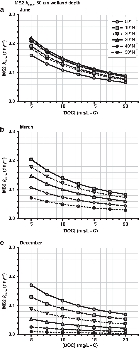
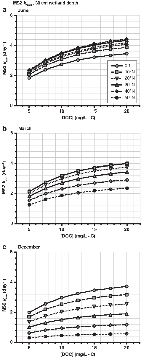
\end{document}) for decay of TrOC, E. coli, and MS2 in a UPOW wetland with a 30-cm depth are presented in Figs. 3–9. In each figure, a range of decay rates are presented for different latitudes, months, [DOC], and pH. Estimated decay rate constants for UPOW wetlands with depths of 20 and 40 cm are presented in Supplementary Figs. S2–S15 of the Supplementary Data, and estimated [1O2]ss are provided in Supplementary Figs. S16–S18 of the Supplementary Data.
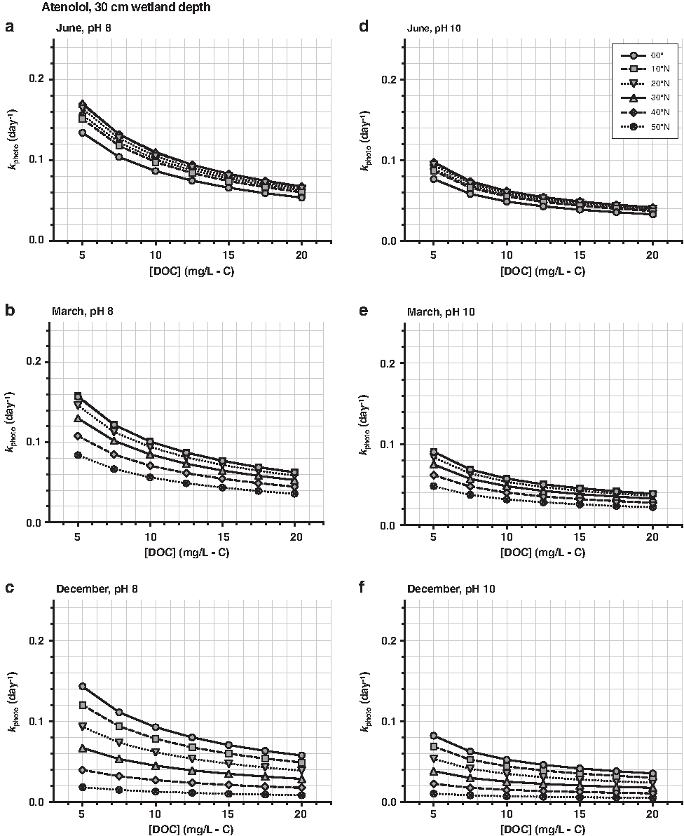
Atenolol phototransformation rates (kphoto; day−1) estimated in an open-water wetland with a 30-cm-deep well-mixed water column. kphoto were estimated for the 21st day of (a, d) June, (b, e) March, and (c, f) December. Choose a [DOC] (mg/L-C), pH, and month to determine kphoto. [\documentclass{aastex}\usepackage{amsbsy}\usepackage{amsfonts}\usepackage{amssymb}\usepackage{bm}\usepackage{mathrsfs}\usepackage{pifont}\usepackage{stmaryrd}\usepackage{textcomp}\usepackage{portland, xspace}\usepackage{amsmath, amsxtra}\usepackage{upgreek}\pagestyle{empty}\DeclareMathSizes{10}{9}{7}{6}\begin{document}
$${{ \rm{NO}}_3^ - }$$
\end{document}] = 10 mg/L-N; [DIC] = 60 mg-C L−1. [DIC], dissolved inorganic carbon concentration.
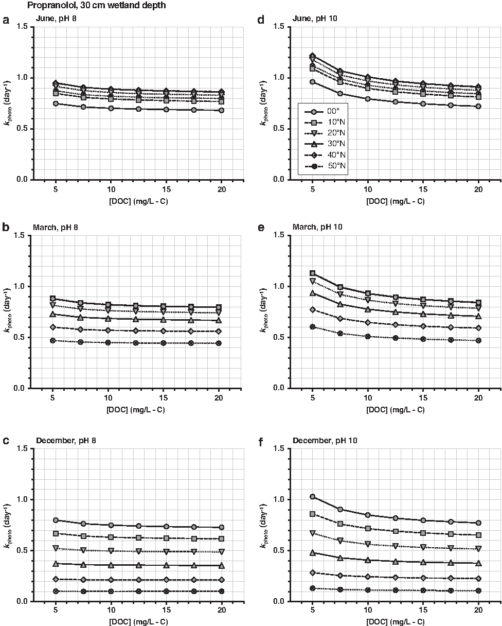
Propranolol phototransformation rates (kphoto; day−1) estimated in an open-water wetland with a 30-cm-deep well-mixed water column. kphoto were estimated for the 21st day of (a, d) June, (b, e) March, and (c, f) December. Choose a [DOC] (mg/L-C), pH, and month to determine kphoto. [\documentclass{aastex}\usepackage{amsbsy}\usepackage{amsfonts}\usepackage{amssymb}\usepackage{bm}\usepackage{mathrsfs}\usepackage{pifont}\usepackage{stmaryrd}\usepackage{textcomp}\usepackage{portland, xspace}\usepackage{amsmath, amsxtra}\usepackage{upgreek}\pagestyle{empty}\DeclareMathSizes{10}{9}{7}{6}\begin{document}
$${{ \rm{NO}}_3^ - }$$
\end{document}] = 10 mg/L-N; [DIC] = 60 mg-C L−1.
Sulfamethoxazole phototransformation rates (kphoto; day−1) estimated in an open-water wetland with a 30-cm-deep well-mixed water column. kphoto were estimated for the 21st day of (a, d) June, (b, e) March, and (c, f) December. Choose a [DOC] (mg/L-C), pH, and month to determine kphoto. [\documentclass{aastex}\usepackage{amsbsy}\usepackage{amsfonts}\usepackage{amssymb}\usepackage{bm}\usepackage{mathrsfs}\usepackage{pifont}\usepackage{stmaryrd}\usepackage{textcomp}\usepackage{portland, xspace}\usepackage{amsmath, amsxtra}\usepackage{upgreek}\pagestyle{empty}\DeclareMathSizes{10}{9}{7}{6}\begin{document}
$${{ \rm{NO}}_3^ - }$$
\end{document}] = 10 mg/L-N; [DIC] = 60 mg-C L−1.
Carbamazepine phototransformation rates (kphoto; day−1) estimated in an open-water wetland with a 30-cm-deep well-mixed water column. kphoto were estimated for the 21st day of (a, d) June, (b, e) March, and (c, f) December. Choose a [DOC] (mg/L-C), pH, and month to determine kphoto. [\documentclass{aastex}\usepackage{amsbsy}\usepackage{amsfonts}\usepackage{amssymb}\usepackage{bm}\usepackage{mathrsfs}\usepackage{pifont}\usepackage{stmaryrd}\usepackage{textcomp}\usepackage{portland, xspace}\usepackage{amsmath, amsxtra}\usepackage{upgreek}\pagestyle{empty}\DeclareMathSizes{10}{9}{7}{6}\begin{document}
$${{ \rm{NO}}_3^ - }$$
\end{document}] = 10 mg/L-N; [DIC] = 60 mg-C L−1.
E. coli endogenous inactivation rates (kendo; day−1) estimated in an open-water wetland with a 30-cm-deep well-mixed water column. kendo were estimated for the 21st day of (a) June, (b) March, and (c) December. Choose a [DOC] (mg-C L−1) and month to determine kendo.
MS2 endogenous inactivation rates (kendo; day−1) estimated in an open-water wetland with a 30-cm-deep well-mixed water column. kendo were estimated for the 21st day of (a) June, (b) March, and (c) December. Choose a [DOC] (mg-C L−1) and month to determine kendo.
MS2 exogenous inactivation rates (kexo; day−1) estimated in an open-water wetland with a 30-cm-deep well-mixed water column. kexo were estimated for the 21st day of (a) June, (b) March, and (c) December. Choose a [DOC] (mg-C L−1) and month to determine kexo.
To calculate total TrOC decay rates, Equation (1) should be used, with \documentclass{aastex}\usepackage{amsbsy}\usepackage{amsfonts}\usepackage{amssymb}\usepackage{bm}\usepackage{mathrsfs}\usepackage{pifont}\usepackage{stmaryrd}\usepackage{textcomp}\usepackage{portland, xspace}\usepackage{amsmath, amsxtra}\usepackage{upgreek}\pagestyle{empty}\DeclareMathSizes{10}{9}{7}{6}\begin{document}
$$k_{{ \rm{photo}}}^i$$
\end{document} read from the figures, and \documentclass{aastex}\usepackage{amsbsy}\usepackage{amsfonts}\usepackage{amssymb}\usepackage{bm}\usepackage{mathrsfs}\usepackage{pifont}\usepackage{stmaryrd}\usepackage{textcomp}\usepackage{portland, xspace}\usepackage{amsmath, amsxtra}\usepackage{upgreek}\pagestyle{empty}\DeclareMathSizes{10}{9}{7}{6}\begin{document}
$$k_{{ \rm{bio}}}^i$$
\end{document} calculated using Equation (2). pH in UPOW wetlands will follow a diurnal cycle, with greatest pH corresponding with maximum sunlight irradiance, due to photosynthesis. Given that TrOC removal due to photolysis occurs when there is sunlight irradiance, the predominant pH during daylight hours should be used when reading the \documentclass{aastex}\usepackage{amsbsy}\usepackage{amsfonts}\usepackage{amssymb}\usepackage{bm}\usepackage{mathrsfs}\usepackage{pifont}\usepackage{stmaryrd}\usepackage{textcomp}\usepackage{portland, xspace}\usepackage{amsmath, amsxtra}\usepackage{upgreek}\pagestyle{empty}\DeclareMathSizes{10}{9}{7}{6}\begin{document}
$$k_{{ \rm{photo}}}^i$$
\end{document} figures. To determine E. coli decay rates, Equation (3) should be used, with \documentclass{aastex}\usepackage{amsbsy}\usepackage{amsfonts}\usepackage{amssymb}\usepackage{bm}\usepackage{mathrsfs}\usepackage{pifont}\usepackage{stmaryrd}\usepackage{textcomp}\usepackage{portland, xspace}\usepackage{amsmath, amsxtra}\usepackage{upgreek}\pagestyle{empty}\DeclareMathSizes{10}{9}{7}{6}\begin{document}
$$k_{{ \rm{endo}}}^i$$
\end{document} read from the figures and \documentclass{aastex}\usepackage{amsbsy}\usepackage{amsfonts}\usepackage{amssymb}\usepackage{bm}\usepackage{mathrsfs}\usepackage{pifont}\usepackage{stmaryrd}\usepackage{textcomp}\usepackage{portland, xspace}\usepackage{amsmath, amsxtra}\usepackage{upgreek}\pagestyle{empty}\DeclareMathSizes{10}{9}{7}{6}\begin{document}
$$k_{{ \rm{dark}}}^{E. \; \;coli}$$
\end{document} equal to 0.86 day−1 (\documentclass{aastex}\usepackage{amsbsy}\usepackage{amsfonts}\usepackage{amssymb}\usepackage{bm}\usepackage{mathrsfs}\usepackage{pifont}\usepackage{stmaryrd}\usepackage{textcomp}\usepackage{portland, xspace}\usepackage{amsmath, amsxtra}\usepackage{upgreek}\pagestyle{empty}\DeclareMathSizes{10}{9}{7}{6}\begin{document}
$$k_{{ \rm{exo}}}^i$$
\end{document} for E. coli is equal to zero). To determine MS2 decay rates, Equation (3) should be used, with \documentclass{aastex}\usepackage{amsbsy}\usepackage{amsfonts}\usepackage{amssymb}\usepackage{bm}\usepackage{mathrsfs}\usepackage{pifont}\usepackage{stmaryrd}\usepackage{textcomp}\usepackage{portland, xspace}\usepackage{amsmath, amsxtra}\usepackage{upgreek}\pagestyle{empty}\DeclareMathSizes{10}{9}{7}{6}\begin{document}
$$k_{{ \rm{endo}}}^i$$
\end{document} and \documentclass{aastex}\usepackage{amsbsy}\usepackage{amsfonts}\usepackage{amssymb}\usepackage{bm}\usepackage{mathrsfs}\usepackage{pifont}\usepackage{stmaryrd}\usepackage{textcomp}\usepackage{portland, xspace}\usepackage{amsmath, amsxtra}\usepackage{upgreek}\pagestyle{empty}\DeclareMathSizes{10}{9}{7}{6}\begin{document}
$$k_{{ \rm{exo}}}^i$$
\end{document} read from the figures (\documentclass{aastex}\usepackage{amsbsy}\usepackage{amsfonts}\usepackage{amssymb}\usepackage{bm}\usepackage{mathrsfs}\usepackage{pifont}\usepackage{stmaryrd}\usepackage{textcomp}\usepackage{portland, xspace}\usepackage{amsmath, amsxtra}\usepackage{upgreek}\pagestyle{empty}\DeclareMathSizes{10}{9}{7}{6}\begin{document}
$$k_{{ \rm{dark}}}^i$$
\end{document} for MS2 is equal to zero).
There are limitations to the model predictions presented in this article. First, although the photolysis and photoinactivation rate model equations represent well-studied mechanisms, and therefore are broadly applicable across sunlit waters, some of the input parameters for the decay rate equations (i.e., [DIC], \documentclass{aastex}\usepackage{amsbsy}\usepackage{amsfonts}\usepackage{amssymb}\usepackage{bm}\usepackage{mathrsfs}\usepackage{pifont}\usepackage{stmaryrd}\usepackage{textcomp}\usepackage{portland, xspace}\usepackage{amsmath, amsxtra}\usepackage{upgreek}\pagestyle{empty}\DeclareMathSizes{10}{9}{7}{6}\begin{document}
$$\left[ {{ \rm{NO}}_3^ - } \right]$$
\end{document}, \documentclass{aastex}\usepackage{amsbsy}\usepackage{amsfonts}\usepackage{amssymb}\usepackage{bm}\usepackage{mathrsfs}\usepackage{pifont}\usepackage{stmaryrd}\usepackage{textcomp}\usepackage{portland, xspace}\usepackage{amsmath, amsxtra}\usepackage{upgreek}\pagestyle{empty}\DeclareMathSizes{10}{9}{7}{6}\begin{document}
$$k_2^i$$
\end{document}, and \documentclass{aastex}\usepackage{amsbsy}\usepackage{amsfonts}\usepackage{amssymb}\usepackage{bm}\usepackage{mathrsfs}\usepackage{pifont}\usepackage{stmaryrd}\usepackage{textcomp}\usepackage{portland, xspace}\usepackage{amsmath, amsxtra}\usepackage{upgreek}\pagestyle{empty}\DeclareMathSizes{10}{9}{7}{6}\begin{document}
$$k_{{ \rm{dark}}}^{E. \; \;coli}$$
\end{document}) were measured in water from the Discovery Bay UPOW wetland and may differ in systems with different water quality. Second, the Discovery Bay and Prado UPOW wetlands had [DOC] of ∼8 and 4.5 mg-C L−1, respectively (Jasper and Sedlak, 2013; Bear et al., 2017), and the decay rate equations have therefore not been validated for the entire [DOC] range modeled in this article. Additionally, the sunlight spectra predicted by SMARTS as inputs to photodegradation equations do not account for atmospheric conditions that would attenuate light in the atmosphere and are therefore assumed to represent clear-sky (e.g., cloud-, haze- and smog-free) conditions. Previous validation of model estimates was conducted in temperate regions, and the effects of freezing temperatures and ice formation during winter at high latitudes is not accounted for in the decay rate predictions.
Sensitivity analysis to screen for important inputs to TrOC removal equations
A one-at-a-time sensitivity analysis was conducted to determine the importance of each model input (i.e., pH, [DOC], [DIC], depth, [NO3−], and temperature) for the calculation of \documentclass{aastex}\usepackage{amsbsy}\usepackage{amsfonts}\usepackage{amssymb}\usepackage{bm}\usepackage{mathrsfs}\usepackage{pifont}\usepackage{stmaryrd}\usepackage{textcomp}\usepackage{portland, xspace}\usepackage{amsmath, amsxtra}\usepackage{upgreek}\pagestyle{empty}\DeclareMathSizes{10}{9}{7}{6}\begin{document}
$$k_{{ \rm{TrOC}}}^i$$
\end{document}. The importance of each input differed for each TrOC evaluated; these results are summarized in Table 1 and Supplementary Fig. S19. For example, temperature was the most important variable for atenolol removal given the importance of temperature-dependent biotransformation for this compound (i.e., increased temperature resulted in increased \documentclass{aastex}\usepackage{amsbsy}\usepackage{amsfonts}\usepackage{amssymb}\usepackage{bm}\usepackage{mathrsfs}\usepackage{pifont}\usepackage{stmaryrd}\usepackage{textcomp}\usepackage{portland, xspace}\usepackage{amsmath, amsxtra}\usepackage{upgreek}\pagestyle{empty}\DeclareMathSizes{10}{9}{7}{6}\begin{document}
$$k_{{ \rm{TrOC}}}^{{ \rm{atenolol}}}$$
\end{document}), whereas depth and [DOC] were important inputs for propranolol and sulfamethoxazole removal given their susceptibility to photolysis (i.e., increasing these values resulted in reduced \documentclass{aastex}\usepackage{amsbsy}\usepackage{amsfonts}\usepackage{amssymb}\usepackage{bm}\usepackage{mathrsfs}\usepackage{pifont}\usepackage{stmaryrd}\usepackage{textcomp}\usepackage{portland, xspace}\usepackage{amsmath, amsxtra}\usepackage{upgreek}\pagestyle{empty}\DeclareMathSizes{10}{9}{7}{6}\begin{document}
$$k_{{ \rm{TrOC}}}^{{ \rm{propranolol}}}$$
\end{document} and \documentclass{aastex}\usepackage{amsbsy}\usepackage{amsfonts}\usepackage{amssymb}\usepackage{bm}\usepackage{mathrsfs}\usepackage{pifont}\usepackage{stmaryrd}\usepackage{textcomp}\usepackage{portland, xspace}\usepackage{amsmath, amsxtra}\usepackage{upgreek}\pagestyle{empty}\DeclareMathSizes{10}{9}{7}{6}\begin{document}
$$k_{{ \rm{TrOC}}}^{{ \rm{sulfamethoxazole}}}$$
\end{document} due to a decrease in sunlight available for direct and indirect photolysis). pH was the most important input for carbamazepine transformation given its reliance on steady-state \documentclass{aastex}\usepackage{amsbsy}\usepackage{amsfonts}\usepackage{amssymb}\usepackage{bm}\usepackage{mathrsfs}\usepackage{pifont}\usepackage{stmaryrd}\usepackage{textcomp}\usepackage{portland, xspace}\usepackage{amsmath, amsxtra}\usepackage{upgreek}\pagestyle{empty}\DeclareMathSizes{10}{9}{7}{6}\begin{document}
$$\bullet { \rm{OH}}$$
\end{document} concentration for degradation, which is highly pH dependent (i.e., at elevated pH, [•OH]ss, and therefore \documentclass{aastex}\usepackage{amsbsy}\usepackage{amsfonts}\usepackage{amssymb}\usepackage{bm}\usepackage{mathrsfs}\usepackage{pifont}\usepackage{stmaryrd}\usepackage{textcomp}\usepackage{portland, xspace}\usepackage{amsmath, amsxtra}\usepackage{upgreek}\pagestyle{empty}\DeclareMathSizes{10}{9}{7}{6}\begin{document}
$$k_{{ \rm{TrOC}}}^{{ \rm{carbamazepine}}}$$
\end{document}, are reduced due to an increase in the concentration of CO32− (pKa2,H2CO3 = 10.33), which quenches \documentclass{aastex}\usepackage{amsbsy}\usepackage{amsfonts}\usepackage{amssymb}\usepackage{bm}\usepackage{mathrsfs}\usepackage{pifont}\usepackage{stmaryrd}\usepackage{textcomp}\usepackage{portland, xspace}\usepackage{amsmath, amsxtra}\usepackage{upgreek}\pagestyle{empty}\DeclareMathSizes{10}{9}{7}{6}\begin{document}
$$\bullet { \rm{OH}}$$
\end{document} at a greater rate than is achieved by HCO3−). The pH effect is the opposite for propranolol and sulfamethoxazole, due to their susceptibility to reaction with carbonate radical: propranolol and sulfamethoxazole have faster \documentclass{aastex}\usepackage{amsbsy}\usepackage{amsfonts}\usepackage{amssymb}\usepackage{bm}\usepackage{mathrsfs}\usepackage{pifont}\usepackage{stmaryrd}\usepackage{textcomp}\usepackage{portland, xspace}\usepackage{amsmath, amsxtra}\usepackage{upgreek}\pagestyle{empty}\DeclareMathSizes{10}{9}{7}{6}\begin{document}
$$k_{{ \rm{TrOC}}}^i$$
\end{document} at elevated pH, given greater CO32− concentrations, and therefore greater carbonate radical concentrations, at higher pH.
Model Inputs for Which Each Trace Organic Contaminant Transformation Rate (\documentclass{aastex}\usepackage{amsbsy}\usepackage{amsfonts}\usepackage{amssymb}\usepackage{bm}\usepackage{mathrsfs}\usepackage{pifont}\usepackage{stmaryrd}\usepackage{textcomp}\usepackage{portland, xspace}\usepackage{amsmath, amsxtra}\usepackage{upgreek}\pagestyle{empty}\DeclareMathSizes{10}{9}{7}{6}\begin{document}
$$k_{{ \rm{TrOC}}}^i$$
\end{document}) Was Most Sensitivea
TrOC
First
Second
Third
Atenolol
Temperature (direct)
[DOC] (inverse)
pH (inverse)
Propranolol
Depth (inverse)
pH (direct)
[DOC] (inverse)
Sulfamethoxazole
[DOC] (inverse)
Depth (inverse)
pH (direct)
Carbamazepine
pH (inverse)
[DOC] (inverse)
[DIC] (inverse)
\documentclass{aastex}\usepackage{amsbsy}\usepackage{amsfonts}\usepackage{amssymb}\usepackage{bm}\usepackage{mathrsfs}\usepackage{pifont}\usepackage{stmaryrd}\usepackage{textcomp}\usepackage{portland, xspace}\usepackage{amsmath, amsxtra}\usepackage{upgreek}\pagestyle{empty}\DeclareMathSizes{10}{9}{7}{6}\begin{document}
$$k_{{ \rm{TrOC}}}^i$$
\end{document} were estimated for an incident sunlight spectrum in March at 30°N. The top three most important inputs are listed. Denoted is whether there was a direct relationship between the input and calculated \documentclass{aastex}\usepackage{amsbsy}\usepackage{amsfonts}\usepackage{amssymb}\usepackage{bm}\usepackage{mathrsfs}\usepackage{pifont}\usepackage{stmaryrd}\usepackage{textcomp}\usepackage{portland, xspace}\usepackage{amsmath, amsxtra}\usepackage{upgreek}\pagestyle{empty}\DeclareMathSizes{10}{9}{7}{6}\begin{document}
$$k_{{ \rm{TrOC}}}^i$$
\end{document} (i.e., an increase in the input led to an increase in \documentclass{aastex}\usepackage{amsbsy}\usepackage{amsfonts}\usepackage{amssymb}\usepackage{bm}\usepackage{mathrsfs}\usepackage{pifont}\usepackage{stmaryrd}\usepackage{textcomp}\usepackage{portland, xspace}\usepackage{amsmath, amsxtra}\usepackage{upgreek}\pagestyle{empty}\DeclareMathSizes{10}{9}{7}{6}\begin{document}
$$k_{{ \rm{TrOC}}}^i$$
\end{document}) or inverse relationship (i.e., an increase in the input led to a decrease in \documentclass{aastex}\usepackage{amsbsy}\usepackage{amsfonts}\usepackage{amssymb}\usepackage{bm}\usepackage{mathrsfs}\usepackage{pifont}\usepackage{stmaryrd}\usepackage{textcomp}\usepackage{portland, xspace}\usepackage{amsmath, amsxtra}\usepackage{upgreek}\pagestyle{empty}\DeclareMathSizes{10}{9}{7}{6}\begin{document}
$$k_{{ \rm{TrOC}}}^i$$
\end{document}, or vice versa).
Results are based on a sensitivity analysis where each input was individually varied by +50% and −50% of its original value.
The following design example is used to illustrate how the framework for estimating contaminant removal rates described in this article can be utilized in conjunction with the P-k-C* equation [Eq. (22)] to design the area (and subsequent volume) of a UPOW wetland to meet water treatment objectives. The P-k-C* equation describes contaminant decay in surface flow wetlands by modeling wetlands as series of well-mixed tanks and including the term C* to account for the background concentration of a compound of interest in the wetland.
In this example, we consider a UPOW wetland used as a polishing step to remove nitrate from wastewater effluent discharged to a sensitive environment in central Florida (e.g., Orlando, 28.5383°N latitude; additional design assumptions are provided in Table 2). The motivation for constructing this UPOW wetland is that effluents from conventional wastewater treatment systems without biological nitrogen removal have nitrate concentrations that range between 10 and 20 mg/L-N, which can lead to nutrient pollution and eutrophication in aquatic environments (Carey and Migliaccio, 2009). We decided to design the system to achieve 90% nitrate removal during the month with median average monthly temperature in Orlando, which is 21.8°C and occurs in April (data from the World Meteorological Organization). Applying Equation (21) with T = 21.8°C resulted in \documentclass{aastex}\usepackage{amsbsy}\usepackage{amsfonts}\usepackage{amssymb}\usepackage{bm}\usepackage{mathrsfs}\usepackage{pifont}\usepackage{stmaryrd}\usepackage{textcomp}\usepackage{portland, xspace}\usepackage{amsmath, amsxtra}\usepackage{upgreek}\pagestyle{empty}\DeclareMathSizes{10}{9}{7}{6}\begin{document}
$${k_{{ \rm{NO}}_3^ - }}$$
\end{document} equal to 72.8 m year−1 (0.20 m day−1). This estimated \documentclass{aastex}\usepackage{amsbsy}\usepackage{amsfonts}\usepackage{amssymb}\usepackage{bm}\usepackage{mathrsfs}\usepackage{pifont}\usepackage{stmaryrd}\usepackage{textcomp}\usepackage{portland, xspace}\usepackage{amsmath, amsxtra}\usepackage{upgreek}\pagestyle{empty}\DeclareMathSizes{10}{9}{7}{6}\begin{document}
$${k_{{ \rm{NO}}_3^ - }}$$
\end{document} is greater than the 90th percentile of nitrate removal rate coefficients identified by Kadlec and Wallace (2009) in a survey of 72 free water surface wetlands.
Assumptions Used to Calculate the Size of the Wetland in the Design Example: Unit Process, Open-Water Wetland in Central Florida During Months with Median Daily Average Temperature and Sunlight Irradiance
For existing systems, tracer tests are used to determine the number of theoretical tanks in series (N) that describes the wetland hydraulics (Kadlec and Wallace, 2009). However, it is not possible to conduct a tracer test in a system that has not yet been designed or constructed. Therefore, for design purposes, N must be estimated. As the flow regime approaches ideal plug flow hydraulics, the number of tanks in series increases. Therefore, treatment system modifications that encourage plug flow—such as using baffles, increasing the length-to-width ratio of the wetland cell or designing the system to have multiple wetland cells in series—will result in a greater value of N. Kadlec and Wallace (2009) surveyed studies that report N values for surface flow vegetated wetlands, and found N to range between 0.3 and 10.7, with a mean of 4.1 (standard error = 0.4). Jasper et al. (2014a, 2014b) found N to equal 6.4 in the highly baffled UPOW wetland in Discovery Bay, CA. The UPOW cells in the Prado wetlands did not contain baffles, but were constructed with a length-to-width ratio of 8.2 to promote channelized flow. However, the system was not as successful in reducing hydraulic inefficiencies, and had an average value of N equal to 2.4 (Bear et al., 2017). In this example, we used a value of 4.4 for N, which is the average of N in the Discovery Bay and Prado UPOW wetlands.
The C* term in the P-k-C* model accounts for the background concentration of a compound of interest in the wetland, which could result from decaying biomass or, in the case of fecal indicator organisms, animal excreta introduced to the wetland. Following recommendations from Kadlec and Wallace (2009), we assumed that the C* value for nitrate is zero. C* for TrOC is also assumed to be zero, as there are no sources for these compounds within the wetland (Kadlec and Wallace, 2009). For fecal coliforms, Kadlec and Wallace (2009) stated that wetland systems with high animal activity have C* values that range between 100 and 500 CFU (100 mL)−1; E. coli C* is assumed to be the same. C* values have not been determined for F+ coliphage (i.e., the family of coliphage that MS2 belongs to), but are assumed to be zero, given that F+ coliphage concentrations of some samples from the Discovery Bay wetland (Silverman et al., 2015) and the Prado wetland (Bear et al., 2017) were found to be below the detection limit.
After rearranging the P-k-C* model equation and assuming C* is equal to zero, the following equation was used to solve for the wetland area required for 90% nitrate removal:
\documentclass{aastex}\usepackage{amsbsy}\usepackage{amsfonts}\usepackage{amssymb}\usepackage{bm}\usepackage{mathrsfs}\usepackage{pifont}\usepackage{stmaryrd}\usepackage{textcomp}\usepackage{portland, xspace}\usepackage{amsmath, amsxtra}\usepackage{upgreek}\pagestyle{empty}\DeclareMathSizes{10}{9}{7}{6}\begin{document}
\begin{align*}
A = { \frac { NQ } { { k_A } } } \left[ { { { \left( { { \frac { { C_ { { \rm { in } } } } } { { C_ { { \rm { out } } } } } } } \right) } ^ { \frac { 1 } { N } } } - 1 } \right] \; \; \;\; OR \; \; \; \; { \frac { NQ } { { k_V } \;z } } \left[ { { { \left( { { \frac { { C_ { { \rm { in } } } } } { { C_ { { \rm { out } } } } } } } \right) } ^ { \frac { 1 } { N } } } - 1 } \right] \tag { 23 }
\end{align*}
\end{document}
Assuming a design flow rate (Q) of 1 MGD (3785.4 m3 day−1), Cout = 0.1 × Cin (i.e., 90% removal), and kA = \documentclass{aastex}\usepackage{amsbsy}\usepackage{amsfonts}\usepackage{amssymb}\usepackage{bm}\usepackage{mathrsfs}\usepackage{pifont}\usepackage{stmaryrd}\usepackage{textcomp}\usepackage{portland, xspace}\usepackage{amsmath, amsxtra}\usepackage{upgreek}\pagestyle{empty}\DeclareMathSizes{10}{9}{7}{6}\begin{document}
$${k_{{ \rm{NO}}_3^ - }}$$
\end{document} = 0.20 m day−1, the required wetland area was estimated to be 57,400 m2 (5.74 ha). Assuming per capita wastewater production of 100 gallons per day, 1 MGD would be the wastewater produced by 10,000 people, and the required wetland area would be 5.74 m2 per person served. While the wetland depth was not needed for this calculation, we assumed a design depth of 30 cm for subsequent calculations.
After considering nitrate removal, we evaluated additional water treatment benefits provided through removal of TrOC and microbial contaminants in the UPOW wetland. This was conducted by first calculating \documentclass{aastex}\usepackage{amsbsy}\usepackage{amsfonts}\usepackage{amssymb}\usepackage{bm}\usepackage{mathrsfs}\usepackage{pifont}\usepackage{stmaryrd}\usepackage{textcomp}\usepackage{portland, xspace}\usepackage{amsmath, amsxtra}\usepackage{upgreek}\pagestyle{empty}\DeclareMathSizes{10}{9}{7}{6}\begin{document}
$$k_{{ \rm{TrOC}}}^i$$
\end{document} and \documentclass{aastex}\usepackage{amsbsy}\usepackage{amsfonts}\usepackage{amssymb}\usepackage{bm}\usepackage{mathrsfs}\usepackage{pifont}\usepackage{stmaryrd}\usepackage{textcomp}\usepackage{portland, xspace}\usepackage{amsmath, amsxtra}\usepackage{upgreek}\pagestyle{empty}\DeclareMathSizes{10}{9}{7}{6}\begin{document}
$$k_{{ \rm{microbial}}}^i$$
\end{document} using Equations (1–3), and the figures provided herein to determine values of \documentclass{aastex}\usepackage{amsbsy}\usepackage{amsfonts}\usepackage{amssymb}\usepackage{bm}\usepackage{mathrsfs}\usepackage{pifont}\usepackage{stmaryrd}\usepackage{textcomp}\usepackage{portland, xspace}\usepackage{amsmath, amsxtra}\usepackage{upgreek}\pagestyle{empty}\DeclareMathSizes{10}{9}{7}{6}\begin{document}
$$k_{{ \rm{photo}}}^i$$
\end{document}, \documentclass{aastex}\usepackage{amsbsy}\usepackage{amsfonts}\usepackage{amssymb}\usepackage{bm}\usepackage{mathrsfs}\usepackage{pifont}\usepackage{stmaryrd}\usepackage{textcomp}\usepackage{portland, xspace}\usepackage{amsmath, amsxtra}\usepackage{upgreek}\pagestyle{empty}\DeclareMathSizes{10}{9}{7}{6}\begin{document}
$$k_{{ \rm{endo}}}^i$$
\end{document}, and \documentclass{aastex}\usepackage{amsbsy}\usepackage{amsfonts}\usepackage{amssymb}\usepackage{bm}\usepackage{mathrsfs}\usepackage{pifont}\usepackage{stmaryrd}\usepackage{textcomp}\usepackage{portland, xspace}\usepackage{amsmath, amsxtra}\usepackage{upgreek}\pagestyle{empty}\DeclareMathSizes{10}{9}{7}{6}\begin{document}
$$k_{{ \rm{exo}}}^i$$
\end{document}. For these calculations, we assumed a [DOC] of 7.5 mg-C L−1 and pH of 8, both of which are in the range observed in wastewater effluent polishing wetlands (e.g., the Discovery Bay UPOW wetland) (Jasper and Sedlak, 2013; Nguyen et al., 2015; Silverman et al., 2015). Photodegradation rates were estimated for the month of March, to give a median estimate of the extent of TrOC and microbial contaminant removal; alternatively, for the northern hemisphere, one could model photodegradation in December or June to estimate minimum or maximum \documentclass{aastex}\usepackage{amsbsy}\usepackage{amsfonts}\usepackage{amssymb}\usepackage{bm}\usepackage{mathrsfs}\usepackage{pifont}\usepackage{stmaryrd}\usepackage{textcomp}\usepackage{portland, xspace}\usepackage{amsmath, amsxtra}\usepackage{upgreek}\pagestyle{empty}\DeclareMathSizes{10}{9}{7}{6}\begin{document}
$$k_{{ \rm{TrOC}}}^i$$
\end{document} and \documentclass{aastex}\usepackage{amsbsy}\usepackage{amsfonts}\usepackage{amssymb}\usepackage{bm}\usepackage{mathrsfs}\usepackage{pifont}\usepackage{stmaryrd}\usepackage{textcomp}\usepackage{portland, xspace}\usepackage{amsmath, amsxtra}\usepackage{upgreek}\pagestyle{empty}\DeclareMathSizes{10}{9}{7}{6}\begin{document}
$$k_{{ \rm{microbial}}}^i$$
\end{document}, respectively.
To illustrate the calculation of \documentclass{aastex}\usepackage{amsbsy}\usepackage{amsfonts}\usepackage{amssymb}\usepackage{bm}\usepackage{mathrsfs}\usepackage{pifont}\usepackage{stmaryrd}\usepackage{textcomp}\usepackage{portland, xspace}\usepackage{amsmath, amsxtra}\usepackage{upgreek}\pagestyle{empty}\DeclareMathSizes{10}{9}{7}{6}\begin{document}
$$k_{{ \rm{TrOC}}}^i$$
\end{document} [Eq. (1)], we estimated the degradation rate of propranolol. First, \documentclass{aastex}\usepackage{amsbsy}\usepackage{amsfonts}\usepackage{amssymb}\usepackage{bm}\usepackage{mathrsfs}\usepackage{pifont}\usepackage{stmaryrd}\usepackage{textcomp}\usepackage{portland, xspace}\usepackage{amsmath, amsxtra}\usepackage{upgreek}\pagestyle{empty}\DeclareMathSizes{10}{9}{7}{6}\begin{document}
$$k_{{ \rm{photo}}}^{{ \rm{propranolol}}}$$
\end{document} in March in 30-cm-deep water with a pH of 8 was read off of Fig. 4b. This was done by locating the intersection between the line for 30°N (close to Orlando's latitude of 28.5383°N) and the x-axis value of [DOC] = 7.5 mg-C L−1; the corresponding y-axis value of 0.7 day−1 represents \documentclass{aastex}\usepackage{amsbsy}\usepackage{amsfonts}\usepackage{amssymb}\usepackage{bm}\usepackage{mathrsfs}\usepackage{pifont}\usepackage{stmaryrd}\usepackage{textcomp}\usepackage{portland, xspace}\usepackage{amsmath, amsxtra}\usepackage{upgreek}\pagestyle{empty}\DeclareMathSizes{10}{9}{7}{6}\begin{document}
$$k_{{ \rm{photo}}}^{{ \rm{propranolol}}}$$
\end{document} (\documentclass{aastex}\usepackage{amsbsy}\usepackage{amsfonts}\usepackage{amssymb}\usepackage{bm}\usepackage{mathrsfs}\usepackage{pifont}\usepackage{stmaryrd}\usepackage{textcomp}\usepackage{portland, xspace}\usepackage{amsmath, amsxtra}\usepackage{upgreek}\pagestyle{empty}\DeclareMathSizes{10}{9}{7}{6}\begin{document}
$$k_{{ \rm{TrOC}}}^i$$
\end{document} for 20 and 40 cm depths are provided in separate figures in the Supplementary Data). Second, \documentclass{aastex}\usepackage{amsbsy}\usepackage{amsfonts}\usepackage{amssymb}\usepackage{bm}\usepackage{mathrsfs}\usepackage{pifont}\usepackage{stmaryrd}\usepackage{textcomp}\usepackage{portland, xspace}\usepackage{amsmath, amsxtra}\usepackage{upgreek}\pagestyle{empty}\DeclareMathSizes{10}{9}{7}{6}\begin{document}
$$k_{{ \rm{bio}}}^i$$
\end{document} was calculated according to Equation (2) using the average air temperature in March in Orlando as an input and was found to be 0.26 day−1. The resulting \documentclass{aastex}\usepackage{amsbsy}\usepackage{amsfonts}\usepackage{amssymb}\usepackage{bm}\usepackage{mathrsfs}\usepackage{pifont}\usepackage{stmaryrd}\usepackage{textcomp}\usepackage{portland, xspace}\usepackage{amsmath, amsxtra}\usepackage{upgreek}\pagestyle{empty}\DeclareMathSizes{10}{9}{7}{6}\begin{document}
$$k_{{ \rm{TrOC}}}^{{ \rm{propranolol}}}$$
\end{document} (0.96 day−1) was then used as an input to the volumetric P-K-C* model [Eq. (22)]; additional inputs were the surface area calculated above (A = 57,400 m2), the depth (z) equal to 0.3 m, and Q, N, and C* as described above. The resulting Cin/Cout was estimated to be 0.048, which corresponds to a 95.2% reduction in the concentration of propranolol in the proposed UPOW wetland.
To estimate E. coli removal, \documentclass{aastex}\usepackage{amsbsy}\usepackage{amsfonts}\usepackage{amssymb}\usepackage{bm}\usepackage{mathrsfs}\usepackage{pifont}\usepackage{stmaryrd}\usepackage{textcomp}\usepackage{portland, xspace}\usepackage{amsmath, amsxtra}\usepackage{upgreek}\pagestyle{empty}\DeclareMathSizes{10}{9}{7}{6}\begin{document}
$$k_{{ \rm{microbial}}}^{E. \;coli}$$
\end{document} was calculated by first reading \documentclass{aastex}\usepackage{amsbsy}\usepackage{amsfonts}\usepackage{amssymb}\usepackage{bm}\usepackage{mathrsfs}\usepackage{pifont}\usepackage{stmaryrd}\usepackage{textcomp}\usepackage{portland, xspace}\usepackage{amsmath, amsxtra}\usepackage{upgreek}\pagestyle{empty}\DeclareMathSizes{10}{9}{7}{6}\begin{document}
$$k_{{ \rm{endo}}}^{E. \;coli}$$
\end{document} off of Fig. 7b; this was done in the same manner as for \documentclass{aastex}\usepackage{amsbsy}\usepackage{amsfonts}\usepackage{amssymb}\usepackage{bm}\usepackage{mathrsfs}\usepackage{pifont}\usepackage{stmaryrd}\usepackage{textcomp}\usepackage{portland, xspace}\usepackage{amsmath, amsxtra}\usepackage{upgreek}\pagestyle{empty}\DeclareMathSizes{10}{9}{7}{6}\begin{document}
$$k_{{ \rm{photo}}}^{{ \rm{propranolol}}}$$
\end{document}. \documentclass{aastex}\usepackage{amsbsy}\usepackage{amsfonts}\usepackage{amssymb}\usepackage{bm}\usepackage{mathrsfs}\usepackage{pifont}\usepackage{stmaryrd}\usepackage{textcomp}\usepackage{portland, xspace}\usepackage{amsmath, amsxtra}\usepackage{upgreek}\pagestyle{empty}\DeclareMathSizes{10}{9}{7}{6}\begin{document}
$$k_{{ \rm{endo}}}^{E. \;coli}$$
\end{document} was estimated to be 1.4 day−1. E. coli is susceptible to dark inactivation, but not to exogenous photoinactivation. Therefore \documentclass{aastex}\usepackage{amsbsy}\usepackage{amsfonts}\usepackage{amssymb}\usepackage{bm}\usepackage{mathrsfs}\usepackage{pifont}\usepackage{stmaryrd}\usepackage{textcomp}\usepackage{portland, xspace}\usepackage{amsmath, amsxtra}\usepackage{upgreek}\pagestyle{empty}\DeclareMathSizes{10}{9}{7}{6}\begin{document}
$$k_{{ \rm{dark}}}^{E.coli}$$
\end{document} was set equal to 0.86 day−1 and \documentclass{aastex}\usepackage{amsbsy}\usepackage{amsfonts}\usepackage{amssymb}\usepackage{bm}\usepackage{mathrsfs}\usepackage{pifont}\usepackage{stmaryrd}\usepackage{textcomp}\usepackage{portland, xspace}\usepackage{amsmath, amsxtra}\usepackage{upgreek}\pagestyle{empty}\DeclareMathSizes{10}{9}{7}{6}\begin{document}
$$k_{{ \rm{exo}}}^{E.coli}$$
\end{document} was set equal to zero. These terms were input to the equation for \documentclass{aastex}\usepackage{amsbsy}\usepackage{amsfonts}\usepackage{amssymb}\usepackage{bm}\usepackage{mathrsfs}\usepackage{pifont}\usepackage{stmaryrd}\usepackage{textcomp}\usepackage{portland, xspace}\usepackage{amsmath, amsxtra}\usepackage{upgreek}\pagestyle{empty}\DeclareMathSizes{10}{9}{7}{6}\begin{document}
$$k_{{ \rm{microbial}}}^{E. \;coli}$$
\end{document} [Eq. (3)], which was estimated to be 2.26 day−1. \documentclass{aastex}\usepackage{amsbsy}\usepackage{amsfonts}\usepackage{amssymb}\usepackage{bm}\usepackage{mathrsfs}\usepackage{pifont}\usepackage{stmaryrd}\usepackage{textcomp}\usepackage{portland, xspace}\usepackage{amsmath, amsxtra}\usepackage{upgreek}\pagestyle{empty}\DeclareMathSizes{10}{9}{7}{6}\begin{document}
$$k_{{ \rm{microbial}}}^{E. \;coli}$$
\end{document} was used as an input to the volumetric P-K-C* model [Eq. (22)] to estimate Cin/Cout as described above for propranolol, but with C* assumed to be equal to 100 CFU/100 mL. Assuming that the E. coli concentration at the inlet of the wetland is 104 CFU/100 mL (Nguyen et al., 2015), the resulting Cin/Cout was calculated to be 0.015, which corresponds to an estimated 98.5% reduction in the concentration of E. coli in the proposed UPOW wetland.
In the above example, we prioritized nitrate removal for UPOW wetland design, and calculated the resulting extent of propranolol and E. coli reduction (see Table 3 for estimated decay rates of all contaminants). If, however, the treatment needs of the wetland require prioritization of TrOC or microbial removal, the design process could be shifted to first calculate \documentclass{aastex}\usepackage{amsbsy}\usepackage{amsfonts}\usepackage{amssymb}\usepackage{bm}\usepackage{mathrsfs}\usepackage{pifont}\usepackage{stmaryrd}\usepackage{textcomp}\usepackage{portland, xspace}\usepackage{amsmath, amsxtra}\usepackage{upgreek}\pagestyle{empty}\DeclareMathSizes{10}{9}{7}{6}\begin{document}
$$k_{{ \rm{TrOC}}}^i$$
\end{document} or \documentclass{aastex}\usepackage{amsbsy}\usepackage{amsfonts}\usepackage{amssymb}\usepackage{bm}\usepackage{mathrsfs}\usepackage{pifont}\usepackage{stmaryrd}\usepackage{textcomp}\usepackage{portland, xspace}\usepackage{amsmath, amsxtra}\usepackage{upgreek}\pagestyle{empty}\DeclareMathSizes{10}{9}{7}{6}\begin{document}
$$k_{{ \rm{microbial}}}^i$$
\end{document}, then use the volumetric form of Equation (22) to calculate the required wetland area. If greater TrOC or microbial removal is desired, it would require a UPOW wetland with a greater surface area or depth to allow for a longer retention time.
Calculated Decay Rates for Design Example: Unit Process, Open-Water Wetland in Central Florida During Months with Median Daily Average Temperature and Sunlight Irradiance
As illustrated above, the simplified modeling approach presented in this study can be used to estimate either the wetland surface area needed to achieve a desired level of contaminant removal or the extent of removal for a given wetland area and hydraulic regime. These estimates should be used as guidance values, because more field data from additional installations are needed to assess variability among UPOW systems. The models presented herein were not formulated to be conservative, but rather attempt to model processes as accurately as possible. Although this approach resulted in relatively good agreement between measured and predicted decay rates, there were some apparent biases in the predictions. For example, carbamazepine decay rates were overpredicted in both the Discovery Bay and Prado UPOW wetlands due to an overestimation of photolysis rates (kobs/kpredicted ∼0.1 at Discovery Bay; Jasper et al., 2014a); atenolol and propranolol decay rates were either over- or underpredicted in the Discovery Bay and Prado UPOW wetlands depending on the month, but generally were predicted within 30% of measured removal rates (Jasper et al., 2014a). There was ∼1:1 agreement between measured and predicted sulfamethoxazole decay rates in sunlight-exposed mesocosms containing Discovery Bay UPOW wetland water (Jasper et al., 2014a). At the Discovery Bay UPOW wetland, the models generally underpredicted E. coli and F+ coliphage decay rates and had average kobs/kpredicted of 3.1 (E. coli; Silverman and Nelson, 2016) and 1.2 (F+ coliphage; Silverman et al., 2015). Appropriate safety factors should be employed by design engineers using best judgment, accounting for how much variability and variance is acceptable for the specific context.
Footnotes
Acknowledgments
This research was supported by the Engineering Research Center for Reinventing the Nations Urban Water Infrastructure (ReNUWIt; Grant EEC-1028968). The authors thank Dr. Justin Jasper, Dr. Mi Nguyen, and Samantha Bear for their dedicated work at the Discovery Bay and Prado wetlands. They thank Virgil Koehne and the staff at the Town of Discovery Bay, and Scott Nygren and the staff of the Prado wetlands (Orange County Water District) for managing the wetlands and their invaluable assistance with research activities. The authors thank Dr. Zackary Jones and Dr. Jonathan Sharp for valuable comments on a previous draft of this article.
Author Disclosure Statement
No competing financial interests exist.
References
1.
BartlettJ.S., CiottiA.M., DavisR.F., and CullenJ.J. (1998). The spectral effects of clouds on solar irradiance. J. Geophys. Res. Oceans, 103, 31017.
2.
BearS.E., NguyenM.T., JasperJ.T., NygrenS., NelsonK.L., and SedlakD.L. (2017). Removal of nutrients, trace organic contaminants, and bacterial indicator organisms in a demonstration-scale unit process open-water treatment wetland. Ecol. Eng., 109, 76.
3.
BloughN.V., and ZeppR.G. (1995). Reactive oxygen species in natural waters. In FooteC.S., Ed., Active Oxygen in Chemistry. Glasgow: Chapman & Hall.
4.
CareyR.O., and MigliaccioK.W. (2009). Contribution of wastewater treatment plant effluents to nutrient dynamics in aquatic systems: A review. Environ. Manage., 44, 205.
5.
CarratalàA., CaladoA.D., MattleM.J., MeierhoferR., LuziS., and KohnT. (2016). Solar disinfection of viruses in polyethylene terephthalate bottles. Appl. Environ. Microbiol., 82, 279.
6.
CunninghamM.L., KrinskyN.I., GiovanazziS.M., and PeakM.J. (1985). Superoxide anion is generated from cellular metabolites by solar radiation and its components. J. Free Radical Biol. Med., 1, 381.
7.
Davies-ColleyR., DonnisonA., and SpeedD. (2000). Towards a mechanistic understanding of pond disinfection. Water Sci. Technol., 42, 149.
8.
Davies-ColleyR., DonnisonA., SpeedD., RossC., and NagelsJ. (1999). Inactivation of faecal indicator microorganisms in waste stabilisation ponds: Interactions of environmental factors with sunlight. Water Res. 33, 1220.
DickensonE.R.V., DrewesJ.E., SedlakD.L., WertE.C., and SnyderS.A. (2009). Applying surrogates and indicators to assess removal efficiency of trace organic chemicals during chemical oxidation of wastewaters. A. Shilton Environ. Sci. Technol., 43, 6242.
11.
DickensonE.R.V., SnyderS.A., SedlakD.L., and DrewesJ.E. (2011). Indicator compounds for assessment of wastewater effluent contributions to flow and water quality. Water Res. 45, 1199.
12.
FisherM.B., IriarteM., and NelsonK.L. (2012). Solar water disinfection (SODIS) of Escherichia coli, Enterococcus spp., and MS2 coliphage: Effects of additives and alternative container materials. Water Res. 46, 1745.
13.
FisherM.B., LoveD.C., SchuechR., and NelsonK.L. (2011). Simulated sunlight action spectra for inactivation of MS2 and PRD1 bacteriophages in clear water. Environ. Sci. Technol., 45, 9249.
14.
GueymardC. (1995). SMARTS2: A Simple Model of the Atmospheric Radiative Transfer of Sunshine: Algorithms and Performance Assessment. Cocoa, FL: Florida Solar Energy Center.
15.
GueymardC.A. (2001). Parameterized transmittance model for direct beam and circumsolar spectral irradiance. Solar Energy. 71, 325.
16.
HaagW.R., and HoigneJ. (1986). Singlet oxygen in surface waters. 3. Photochemical formation and steady-state concentrations in various types of waters. Environ. Sci. Technol. 20, 341.
17.
HambyD.M. (1994). A review of techniques for parameter sensitivity analysis of environmental models. Environ. Monit. Assess., 32, 135.
18.
HoignéJ., FaustB.C., HaagW.R., ScullyF.E., and ZeppR.G. (1988). Aquatic humic substances as sources and sinks of photochemically produced transient reactants. In SuffetI.H. and MacCarthyP., Eds., Aquatic Humic Substances. Washington, DC: American Chemical Society.
19.
JaggerJ. (1985). Solar-UV Actions on Living Cells. New York: Praeger Publishers.
20.
JasperJ.T., JonesZ.L., SharpJ.O., and SedlakD.L. (2014a). Biotransformation of trace organic contaminants in open-water unit process treatment wetlands. Environ. Sci. Technol., 48, 5136.
21.
JasperJ.T., JonesZ.L., SharpJ.O., and SedlakD.L. (2014b). Nitrate removal in shallow, open-water treatment wetlands. Environ. Sci. Technol., 48, 11512.
22.
JasperJ.T., NguyenM.T., JonesZ.L., IsmailN.S., SedlakD.L., SharpJ.O., LuthyR.G., HorneA.J., and NelsonK.L. (2013). Unit process wetlands for removal of trace organic contaminants and pathogens from municipal wastewater effluents. Environ. Eng. Sci., 30, 421.
23.
JasperJ.T., and SedlakD.L. (2013). Phototransformation of wastewater-derived trace organic contaminants in open-water unit process treatment wetlands. Environ. Sci. Technol., 47, 10781.
24.
JonesZ.L., JasperJ.T., SedlakD.L., and SharpJ.O. (2017). Sulfide-induced dissimilatory nitrate reduction to ammonium supports anammox in an open-water unit process wetland. Appl. Environ. Microbiol., 83, e00782.
25.
JonesZ.L., MikkelsonK.M., NygrenS., SedlakD.L., and SharpJ.O. (2018). Establishment and convergence of photosynthetic microbial biomats in shallow unit process open-water wetlands. Water Res. 133, 132.
26.
KadirK. (2010). Sunlight-mediated inactivation mechanisms of Enteroccocus faecalis and Escherichia coli in waste stabilization ponds. Ph.D. Dissertation, University of California, Berkeley, CA.
27.
KadirK., and NelsonK.L. (2014). Sunlight mediated inactivation mechanisms of Enterococcus faecalis and Escherichia coli in clear water versus waste stabilization pond water. Water Res. 50, 307.
KohnT., MattleM.J., MinellaM., and VioneD. (2016). A modeling approach to estimate the solar disinfection of viral indicator organisms in waste stabilization ponds and surface waters. Water Res. 88, 912.
31.
KohnT., and NelsonK.L. (2007). Sunlight-mediated inactivation of MS2 coliphage via exogenous singlet oxygen produced by sensitizers in natural waters. Environ. Sci. Technol., 41, 192.
32.
LoveD.C., SilvermanA., and NelsonK.L. (2010). Human virus and bacteriophage inactivation in clear water by simulated sunlight compared to bacteriophage inactivation at a southern California beach. Environ. Sci. Technol., 44, 6965.
33.
MattleM.J., VioneD., and KohnT. (2015). Conceptual model and experimental framework to determine the contributions of direct and indirect photoreactions to the solar disinfection of MS2, phiX174, and Adenovirus. Environ. Sci. Technol., 49, 334.
34.
NguyenM.T., JasperJ.T., BoehmA.B., and NelsonK.L. (2015). Sunlight inactivation of fecal indicator bacteria in open-water unit process treatment wetlands: Modeling endogenous and exogenous inactivation rates. Water Res. 83, 282.
35.
NguyenM.T., SilvermanA.I., and NelsonK.L. (2014). Sunlight inactivation of MS2 coliphage in the absence of photosensitizers: Modeling the endogenous inactivation rate using a photoaction spectrum. Environ. Sci. Technol., 48, 3891.
36.
PrasseC., WenkJ., JasperJ.T., TernesT.A., and SedlakD.L. (2015). Co-occurrence of photochemical and microbiological transformation processes in open-water unit process wetlands. Environ. Sci. Technol., 49, 14136.
37.
RomeroO.C., StraubA.P., KohnT., and NguyenT.H. (2011). Role of temperature and Suwannee River natural organic matter on inactivation kinetics of Rotavirus and bacteriophage MS2 by solar irradiation. Environ. Sci. Technol., 45, 10385.
38.
Romero-MaracciniO.C., SadikN.J., Rosado-LausellS.L., PughC.R., NiuX.-Z., CrouéJ.-P., and NguyenT.H. (2013). Sunlight-induced inactivation of human Wa and porcine OSU rotaviruses in the presence of exogenous photosensitizers. Environ. Sci. Technol., 47, 11004.
39.
Rosado-LausellS.L., WangH., GutierrezL., Romero-MaracciniO.C., NiuX.-Z., GinK.Y.H., CrouéJ.-P., and NguyenT.H. (2013). Roles of singlet oxygen and triplet excited state of dissolved organic matter formed by different organic matters in bacteriophage MS2 inactivation. Water Res. 47, 4869.
40.
SchwarzenbachR.P., GschwendP.M., and ImbodenD.M. (2003). Environmental Organic Chemistry, 2nd ed. New Jersey: Wiley.
41.
SilvermanA.I., and NelsonK.L. (2016). Modeling the endogenous sunlight inactivation rates of laboratory strain and wastewater-sourced E. coli and enterococci using photoaction spectra. Environ. Sci. Technol., 50, 12292.
42.
SilvermanA.I., NguyenM.T., SchillingI.E., WenkJ., and NelsonK.L. (2015). Sunlight inactivation of viruses in open-water unit process treatment wetlands: Modeling endogenous and exogenous inactivation rates. Environ. Sci. Technol., 49, 2757.
43.
SilvermanA.I., PetersonB.M., BoehmA.B., McNeillK., and NelsonK.L. (2013). Sunlight inactivation of human viruses and bacteriophages in coastal waters containing natural photosensitizers. Environ. Sci. Technol., 47, 1870.
44.
SintonL.W., FinlayR.K., and LynchP.A. (1999). Sunlight inactivation of fecal bacteriophages and bacteria in sewage-polluted seawater. Appl. Environ. Microbiol., 65, 3605.
45.
SintonL.W., HallC.H., LynchP.A., and Davies-ColleyR.J. (2002). Sunlight inactivation of fecal indicator bacteria and bacteriophages from waste stabilization pond effluent in fresh and saline waters. Appl. Environ. Microbiol., 68, 1122.
46.
SnyderS.A., WesterhoffP., YoonY., and SedlakD.L. (2003). Pharmaceuticals, personal care products, and endocrine disruptors in water: Implications for the water industry. Environ. Eng. Sci., 20, 449.
47.
TernesT.A., JossA., and SiegristH. (2004). Peer reviewed: Scrutinizing pharmaceuticals and personal care products in wastewater treatment. Environ. Sci. Technol., 38, 392A.
48.
ZeppR.G. (1988). Environmental photoprocesses involving natural organic matter. In FrimmelF. H. and ChristmanR. F., Eds., Humic Substances and Their Role in the Environment. New Jersey: John Wiley & Sons Ltd.
49.
ZeppR.G., and ClineD.M. (1977). Rates of direct photolysis in aquatic environment. Environ. Sci. Technol., 11, 359.
Supplementary Material
Please find the following supplemental material available below.
For Open Access articles published under a Creative Commons License, all supplemental material carries the same license as the article it is associated with.
For non-Open Access articles published, all supplemental material carries a non-exclusive license, and permission requests for re-use of supplemental material or any part of supplemental material shall be sent directly to the copyright owner as specified in the copyright notice associated with the article.