Reliable Model of Reservoir Water Quality Prediction Based on Improved ARIMA Method

Abstract

With the frequent occurrence of water pollution, the safety of the surface water environment has become increasingly severe. Studying the changing trend of reservoir water quality and establishing a prediction and early warning system for water eutrophication is of great significance to the management and maintenance of water resources. Based on the time series ARIMA model, the Holt-Winters seasonal model was introduced for optimization, and a universal water quality prediction model with eutrophication indicator Total Phosphorus and Total Nitrogen as parameters was established. And through self-correction, the water quality prediction accuracy rate has been improved to 97.5%. Experiments showed that compared with the traditional water quality prediction model, this model is simpler and more convenient, and it has the advantages of high learning speed, high prediction accuracy, easy multi-dimensional analysis of data, and close connection with the development laws of things. Therefore, the model can be applied to the short-term prediction of different reservoirs, can significantly reduce the predicted cost of reservoir water quality, and provide methods for the study of dynamic changes of reservoir water quality parameters; thus, it will be a scientific basis and decision support for water quality improvement.

Introduction

With the frequent occurrence of water pollution, the safety of the surface water environment has become increasingly serious. In the process of regional water environment planning, evaluation, and management, water quality prediction is a basic task. How to predict the change of water quality easily and effectively is an effective way to prevent the deterioration of the surface water quality. In recent years, research projects on water quality prediction methods at home and abroad have been turned into practical applications. The main water quality prediction methods include gray prediction methods, fuzzy cluster analysis methods, regression analysis methods, artificial neural network algorithms, etc.

In addition to the artificial neural network algorithms, the methods cited earlier are mostly suitable for large-scale, low-dimensional data prediction; whereas the prediction effects of nonlinear small-sample, high-dimensional data are not ideal. The neural network algorithm is limited by local optimal value, over-learning, and other issues. For example, the accuracy of the BP neural network model under particle swarm optimization is less than 90% (Xu et al., 2016). In addition, water environment researchers are actively introducing the application of visualization and virtual technology to improve the accuracy of forecasting results. For example, some scholars used the statistical relationship between Advanced Spaceborne Thermal Radiation and reflected radiation (ASTER) data and observed water quality parameters to accurately predict the mathematical relationship of missing data in a specific area, and the prediction accuracy can reach 90% (Abdelmalik, 2016); Some studies of UV-visible spectroscopy (Zhang et al., 2016) used by some scholars have also improved prediction accuracy to a certain extent.

Due to the exploration of water quality prediction methods, influenced by the randomness and accidental effects of the water environment, as well as geographical and environmental factors, some research scholars tend to adopt comprehensive models, for instance, the prediction accuracy of the Mewsub rapid-movement early warning system is above 90% (Wang et al., 2018); the Adaptive Neuro Fuzzy Inference System (ANFIS) is used to simulate and predict total phosphorus (TP) and total nitrogen (TN) in water (Khadr and Elshemy, 2016); some scholars have combined Principal Component Analysis (PCA), Genetic Algorithm (GA), Back Propagation Neural Network (BPNN), and the design of a hybrid intelligent algorithm to predict river water quality (Ding et al., 2014); and another example is Chester Freud Carlson's method of machine learning for the prediction of the nutritional status index using four methods to integrate scenarios to complete the prediction (Chou et al., 2018).

However, other scholars believe that the integrated model will solve the problem of prediction uncertainty caused by excessive accumulation of errors (Orzepowski et al., 2014). Therefore, it is apt to use an optimization model with relatively simple procedures, parameter determination, and relatively simple model correction for predictive analysis; for example, the neural network model of coupled dynamic equations (Guo et al., 2018), the GABP model optimized by the PCA method (Liu et al., 2017), the water quality prediction method based on the LWCA-SVM model with prediction accuracy as high as 90% (Dai et al., 2017), a wavelet neural network prediction model (Zhang et al., 2016), the water quality prediction model based on association vector regression (Avila et al., 2018), etc. To sum up, the selection of the model should be determined by considering the level of the user's cognitive level and the integrity and accuracy of the basic data.

The research team conducted a continuous water quality inspection for Shihe reservoir (Mikalsen et al., 2018), an important water supply reservoir that is located in Qinhuangdao City, Hebei Province, for 5 years, trying to find a simple and effective general-purpose reservoir water quality prediction model. The Shihe reservoir, also known as Yansai Lake, is located in the northwestern part of the Shanhaiguan District of Qinhuangdao City, Hebei Province, and is on the main stream of the lower Shihe river. The reservoir area has beautiful scenery, in which the narrow winding waters are clear and transparent, the peaks of the two sides stand tall, and the hillsides are verdant. It is a medium-sized reservoir that is mainly water supplied and has the combined benefits of irrigation and power generation. The Shihe reservoir plays an important role in human society and economic fields.

However, due to some reasons in recent years, some parameters in the reservoir area are occasionally exceeded. To achieve timely understanding of the status of water quality and prevent the occurrence of water pollution incidents, it is necessary to strengthen supervision and management of water quality and improve water quality forecasting and early warning systems. Because the water quality is affected by natural factors such as seasons, climate, runoff, and other human activities including industrial development and urbanization, and the relationship between the factors is complex and changeable, water environment management becomes very challenging. The analysis of the characteristics of the time series of existing water quality parameters, finding out the laws of water quality changes, and making predictions are the key to solving this problem, and it is also an important basis for making scientific decisions on water environment management (Jaddi and Abdullah, 2017).

To accurately predict eutrophication indicator TP and TN, this article proposes the following model: the autoregressive integrated moving average model (abbreviated ARIMA). The model was proposed by the statisticians Box and Jenkins and has been proved to be a mathematical method that can effectively select lag terms and accurately predict non-stationary time series. The model has been successfully applied in the fields of climate, health care, economic management, and tourism (Bedri et al., 2016). Its advantages are obvious, and the prediction results can be accurate regardless of whether using small or large samples. Considering that most of the reservoir water quality monitoring data usually have large samples, most scholars use an optimized neural network model for processing, and this method is rarely used in water quality prediction.

Therefore, the method proposed in this article is of great significance for predicting the water environment of newly developed reservoirs with only a small amount of monitoring data, and it is of universal significance to the long-term monitoring of the water environment of reservoirs.

The ARIMA model predicts the evolution of reservoir parameters and simulates the evolution trend of TP and TN in reservoirs through linear combinations of self-hysteresis values and stochastic perturbation lag values (Bedri et al., 2016), so as to further calculate the degree of eutrophication of the reservoir. In this article, the optimized time series ARIMA model (Rizo-Decelis et al., 2017) is used to dynamically simulate and predict the content of TP and TN of the reservoir over the past 5 years, getting rid of the shortcomings of the common time series model that neglects external environmental factors, highlighting the importance of seasonal influences, making the development of things more closely linked in the present and future. and further improving the prediction effect of reservoir water quality. This method can simultaneously correct the seasonality and tendency of the series, and, based on the stability and regularity of the time series situation, grasp the variation trend of the past data and explain the variation rule of the prediction.

The purpose of this study is to search for a simple and universal prediction method for improving the accuracy of reservoir prediction, reducing the prediction cost of reservoir water quality, and providing a scientific basis and decision support for water quality improvement. From the results of the study, this article has excellently completed the research objectives and meets expectations.

Materials and Methods

Materials

Analytical-grade reagents used were all purchased from Tianjin chemical reagent factory. The process of sampling was strictly carried out in accordance with Technical Specifications Requirements for Monitoring of Surface Water and Waste Water, sampling in the water supply point of the Shihe reservoir, formulating a detailed sampling plan, and carefully filling in the water quality sampling record table to ensure the quality of the water quality sampling. Water quality test was carried out in the laboratory. The TP was analyzed by the ammonium molybdate spectrophotometry method according to the standard, and the TN was analyzed by the ultraviolet spectrophotometric method with alkaline potassium persulfate digestion (National Standard of the People's Republic of China GB11894-89) (SEPA, 2002). To obtain the most time-representative samples and ensure the accuracy of the experiment, the laboratory sampled three times a month, and the average value was analyzed. The sampling time was fixed from 5 to 10 days a month.

Modeling method

Based on the TP and TN data of the Shihe reservoir from January 2013 to December 2016, the time series ARIMA model was established by using R-Studio software, optimized by the Holt-Winters season model, and verified by the actual data from January to July 2017. The eutrophication degree of the Shihe reservoir was predicted under the premise of ensuring high prediction accuracy.

Time series ARIMA model based on optimized Holt-Winters seasonal model

Introduction of model

The full name of the ARIMA (p, d, q) model is Autoregressive Integrated Moving Average Model, abbreviated ARIMA, in which AR is a self-regression term, p is a self-regression term, MA is the moving average, q is the moving average term, and d is the number of integrations made when the time series is optimized to be stationary. ARIMA refers to the model that converts a non-stationary time series into a stationary time series and then returns the dependent variable only to its lagged value and the present and lag values of the random error term. In the analysis method of non-stationary time series, they can be divided into two categories: deterministic time series analysis and stochastic time series analysis. The methods of extracting information from deterministic time series analysis mainly include trend fitting model, seasonal adjustment model, moving average, index smoothing, and so on. The methods of extracting information from stochastic time series analysis include ARIMA (autoregressive integrated moving average) and heteroscedasticity model of autoregressive conditions. ARIMA is the most common method in current time series analysis. It is a process of analysis after the long-term trend, fixed period, and other information are extracted through difference operation, and the non-stationary sequence is changed into a stationary sequence. After the initial processing of the data, if the data show a clear seasonal variation, it is suitable for ARIMA (p, d, q) (Zhang et al., 2018). In view of this characteristic of data, we introduce the Holt-Winters exponential smoothing method to make a short-term prediction (Liu et al., 2018). This method can correct the seasonal propensity of the sequence at the same time (Lavrenz et al., 2018). Based on the stability and regularity of the time series situation, the change trend of the past data is grasped and the changing rules of the forecast are explained.

Modeling steps

First, the time series of the data was tested, and the original data were processed by differential processing to make the data tend toward static distribution and determine the parameter d in the ARIMA model. Second, our team analyzed the autocorrelation graph auto correlation function (ACF) and the partial autocorrelation graph partial auto correlation function (PACF) generated by the sample to determine the parameter q and the parameter p in the ARIMA model. Finally, the ARIMA function was called to predict and test the data and verified with actual data. If p < 0.05, the residual was a non-white noise sequence in the residual test, which showed that the model can continue to be optimized. Due to the obviously seasonal trend of the data, the Holt-Winters exponential smoothing method was adopted to optimize the data and improved the prediction accuracy of the data so that the accuracy of the prediction result reached 99%.

The specific process is shown in Fig. 1.

FIG. 1.

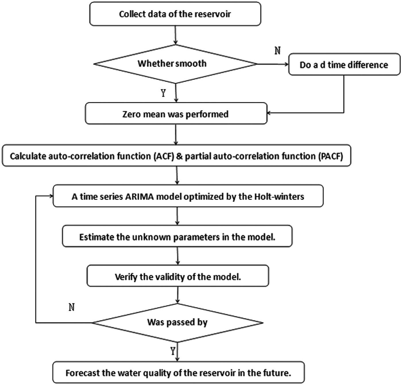
Modeling steps.

Model equations

ARIMA is the combination of two algorithms: AR and MA. The formula was as follows: \documentclass{aastex}\usepackage{amsbsy}\usepackage{amsfonts}\usepackage{amssymb}\usepackage{bm}\usepackage{mathrsfs}\usepackage{pifont}\usepackage{stmaryrd}\usepackage{textcomp}\usepackage{portland, xspace}\usepackage{amsmath, amsxtra}\usepackage{upgreek}\pagestyle{empty}\DeclareMathSizes{10}{9}{7}{6}\begin{document} \begin{align*} {X_t} = c + { \sum \nolimits_{i = 1}^p {{ \phi _i}{X_{t - i}} + \varepsilon } _t} - \sum \nolimits_{i = 1}^q {{ \theta _i}{ \varepsilon _{t - i}}} \tag{1} \end{align*} \end{document}

\documentclass{aastex}\usepackage{amsbsy}\usepackage{amsfonts}\usepackage{amssymb}\usepackage{bm}\usepackage{mathrsfs}\usepackage{pifont}\usepackage{stmaryrd}\usepackage{textcomp}\usepackage{portland, xspace}\usepackage{amsmath, amsxtra}\usepackage{upgreek}\pagestyle{empty}\DeclareMathSizes{10}{9}{7}{6}\begin{document} $${ \varepsilon _t}$$ \end{document} was white noise, the average value was 0, and C was a constant.

The first half of ARIMA was Autoregressive: \documentclass{aastex}\usepackage{amsbsy}\usepackage{amsfonts}\usepackage{amssymb}\usepackage{bm}\usepackage{mathrsfs}\usepackage{pifont}\usepackage{stmaryrd}\usepackage{textcomp}\usepackage{portland, xspace}\usepackage{amsmath, amsxtra}\usepackage{upgreek}\pagestyle{empty}\DeclareMathSizes{10}{9}{7}{6}\begin{document} \begin{align*} {X_t} = c + { \sum \nolimits_{i = 1}^p {{ \phi _i}{X_{i - i}} + \varepsilon } _t} \tag{2} \end{align*} \end{document}

The second half was moving average: \documentclass{aastex}\usepackage{amsbsy}\usepackage{amsfonts}\usepackage{amssymb}\usepackage{bm}\usepackage{mathrsfs}\usepackage{pifont}\usepackage{stmaryrd}\usepackage{textcomp}\usepackage{portland, xspace}\usepackage{amsmath, amsxtra}\usepackage{upgreek}\pagestyle{empty}\DeclareMathSizes{10}{9}{7}{6}\begin{document} \begin{align*} {X_t} = \mu + { \varepsilon _t} - \sum \nolimits_{i = 1}^p {{ \phi _i}} { \varepsilon _{t - i}} \tag{3} \end{align*} \end{document}

AR was actually an infinite impulse response filter, MA was a finite impulse response, and the input was white noise.

I in the ARIMA refers to Integrated; ARIMA (p, d, q) denotes p-order AR, d-time difference, and q-order MA. This article adopts the form of difference. At this point, the number of difference is the order d in the ARIMA (p, d, q) model. In the process of difference operation, the higher the order is, the better. The process of difference operation is the process of information processing and extraction. Therefore, the general difference number is no more than two times. After the time series data are stabilized, the ARIMA (p, d, q) model is transformed into the ARMA (p, q) model.

The time series predicted by the Holt-Winters exponential smoothing method was y_t; the equation for the smoothed sequence \documentclass{aastex}\usepackage{amsbsy}\usepackage{amsfonts}\usepackage{amssymb}\usepackage{bm}\usepackage{mathrsfs}\usepackage{pifont}\usepackage{stmaryrd}\usepackage{textcomp}\usepackage{portland, xspace}\usepackage{amsmath, amsxtra}\usepackage{upgreek}\pagestyle{empty}\DeclareMathSizes{10}{9}{7}{6}\begin{document} $${y^\prime _t}$$ \end{document} was as follows: \documentclass{aastex}\usepackage{amsbsy}\usepackage{amsfonts}\usepackage{amssymb}\usepackage{bm}\usepackage{mathrsfs}\usepackage{pifont}\usepackage{stmaryrd}\usepackage{textcomp}\usepackage{portland, xspace}\usepackage{amsmath, amsxtra}\usepackage{upgreek}\pagestyle{empty}\DeclareMathSizes{10}{9}{7}{6}\begin{document} \begin{align*} {y ^\prime _{t + k}} = {a_t} + {b_t}k + {c_{t + k}} \tag{4} \end{align*} \end{document}

The formula for a,b,c was as follows: \documentclass{aastex}\usepackage{amsbsy}\usepackage{amsfonts}\usepackage{amssymb}\usepackage{bm}\usepackage{mathrsfs}\usepackage{pifont}\usepackage{stmaryrd}\usepackage{textcomp}\usepackage{portland, xspace}\usepackage{amsmath, amsxtra}\usepackage{upgreek}\pagestyle{empty}\DeclareMathSizes{10}{9}{7}{6}\begin{document} \begin{align*} {a_t} = \alpha ( {y_t} - {c_{t - s}} ) + ( 1 - a ) ( {a_{t - 1}} + {c_{t - 1}} ) \tag{5} \end{align*} \end{document} \documentclass{aastex}\usepackage{amsbsy}\usepackage{amsfonts}\usepackage{amssymb}\usepackage{bm}\usepackage{mathrsfs}\usepackage{pifont}\usepackage{stmaryrd}\usepackage{textcomp}\usepackage{portland, xspace}\usepackage{amsmath, amsxtra}\usepackage{upgreek}\pagestyle{empty}\DeclareMathSizes{10}{9}{7}{6}\begin{document} \begin{align*} {b_t} = \beta ( {a_t} - {a_{t - 1}} ) + ( 1 - \beta ) {b_{t - 1}} \tag{6} \end{align*} \end{document} \documentclass{aastex}\usepackage{amsbsy}\usepackage{amsfonts}\usepackage{amssymb}\usepackage{bm}\usepackage{mathrsfs}\usepackage{pifont}\usepackage{stmaryrd}\usepackage{textcomp}\usepackage{portland, xspace}\usepackage{amsmath, amsxtra}\usepackage{upgreek}\pagestyle{empty}\DeclareMathSizes{10}{9}{7}{6}\begin{document} \begin{align*} {c_t} = \gamma ( {y_t} - {a_t} ) + ( 1 - \gamma ) {c_{t - s}} \tag{7} \end{align*} \end{document}

Predictive value calculation formula: \documentclass{aastex}\usepackage{amsbsy}\usepackage{amsfonts}\usepackage{amssymb}\usepackage{bm}\usepackage{mathrsfs}\usepackage{pifont}\usepackage{stmaryrd}\usepackage{textcomp}\usepackage{portland, xspace}\usepackage{amsmath, amsxtra}\usepackage{upgreek}\pagestyle{empty}\DeclareMathSizes{10}{9}{7}{6}\begin{document} \begin{align*} {y ^\prime _{r + k}} = {a_r} + {b_r}k + {c_{r + k - s}} \tag{8} \end{align*} \end{document}

In the formula just cited, a denotes overall smoothness; b denotes smooth trend; c denotes seasonal smoothness, t = 1,2,…T; k denotes the number of post-smoothing periods, k > 0; \documentclass{aastex}\usepackage{amsbsy}\usepackage{amsfonts}\usepackage{amssymb}\usepackage{bm}\usepackage{mathrsfs}\usepackage{pifont}\usepackage{stmaryrd}\usepackage{textcomp}\usepackage{portland, xspace}\usepackage{amsmath, amsxtra}\usepackage{upgreek}\pagestyle{empty}\DeclareMathSizes{10}{9}{7}{6}\begin{document} $$\alpha , \beta , \gamma$$ \end{document} denotes post-smoothing parameter, \documentclass{aastex}\usepackage{amsbsy}\usepackage{amsfonts}\usepackage{amssymb}\usepackage{bm}\usepackage{mathrsfs}\usepackage{pifont}\usepackage{stmaryrd}\usepackage{textcomp}\usepackage{portland, xspace}\usepackage{amsmath, amsxtra}\usepackage{upgreek}\pagestyle{empty}\DeclareMathSizes{10}{9}{7}{6}\begin{document} $$\varepsilon [ 0 , 1 ]$$ \end{document} ; and s is seasonal length, for monthly data s = 12. The weight of the optimization of some commonly used methods include: using the neural network, using the forward selection of learners, selection with replacement, and bagging of ensemble methods.

Stationarity can be tested by using the sequence diagram Argument Dikey-Fuler Test.

-AR is a trailing sequence, that is, the calculated value of ACF is related to the autocorrelation function of order 1 to order p lag, no matter how big k is taken in the lag period.

-AR is the truncated sequence, that is, when the lag period is k>p, PACF = 0.

Statistical tools

Excel spreadsheets were used to establish a database of TP and TN, and R-Studio software was used to model and analyze the data.

Results and Discussion

Analysis and prediction of water quality factors

The feature analysis of TP and TN

According to Fig. 2, from 2013 to 2016, the content of TP of Shihe reservoir had the following trends. The data showed volatility changes. The regularity and seasonality of the sample data was not obvious.

FIG. 2.

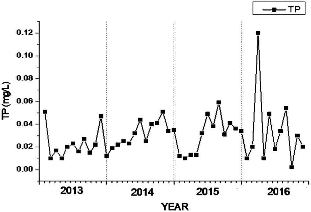
Timing chart of changes in TP data (each point was the monthly average). TP, total phosphorus.

According to Fig. 3, the content of TN had the following trends. The sample data are very volatile. The variance of the sample data is large. The seasonal factor is not obvious.

FIG. 3.

Timing chart of changes in TN data (each point was monthly average). TN, total nitrogen.

After a comprehensive analysis, our team believed that the reasons for the trend just cited were as follows: The data were insufficient, so they cannot show the obvious trend; the data were not preprocessed; and there were interference data.

Time series ARMA model modeling based on Holt-Winters seasonal model optimization

The time series of the test data and the original data were subjected to an integrated process so that the data tended to be statically distributed.

Our team viewed the sample-generated autocorrelation graph ACF and partial autocorrelation map PACF to determine the parameters q and p in the ARIMA model. We selected the main influencing factors to study the seasonal trend and revised the relevant data.

From Fig. 4, it can be seen that after excluding the influence of the data itself, the TP partial autocorrelation coefficient decays to zero in some way, making the data tending to be stable. Then, we do the stationarity test: observation and unit root test.

FIG. 4.

Autocorrelation and partial autocorrelation of TP data.

From Fig. 5, similarly, after excluding the influence of the data itself, the partial nitrogen autocorrelation coefficient also decays to zero in some way, so that the data tend to be stable. Then, we do the stationarity test: observation and unit root test.

FIG. 5.

Autocorrelation and partial autocorrelation of TN Data.

The ARIMA function was called to perform prediction and error checking on the data and verify them with actual data.

After performing the integrated processing, the ARIMA function was called to process the data. As can be seen from Fig. 6, the data had a clear seasonal trend. Periodicity can be tested by using regular sequences or Fourier transforms. If the sampling is not regular, consider Lomb analysis. The core of checking periodicity is analyzing the spatial characteristics of the frequency domain.

FIG. 6.

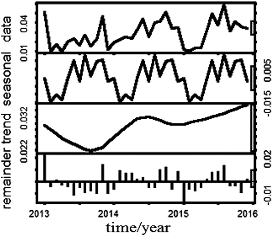
Periodicity of TP.

In recent years, the TP content of the Shihe reservoir had shown an upward trend. This was closely connected with the instability of environmental climate in recent years, and the development of industrialization had caused certain damage to the environment, resulting in the pollution of the water quality. If it was not dealt with as soon as possible, it would lead to much more serious consequences.

According to Fig. 7, similarly, after integrated processing, the TN data also showed a distinct seasonal trend; however, its overall trend decreased first and then increased. Compared with TP, the TN content in the Shihe reservoir increased later, but the rise was faster. The air contained a large amount of nitrogen elements. If the conditions were right, it was likely that some elements in the water can reflect the formation of nitrate that can be dissolved in water.

FIG. 7.

Periodic law of TN.

Next, we introduce the Holt-Winters seasonal model to optimize the time series ARIMA model. The results are as follows:

From Figs. 8 and 9, it can be seen that red was the sample data, green was the raw data fitting value calculated from the sample data, and the blue segment was the predicted value. It can be seen that there was almost no difference, and the prediction effect is also very great. From the previous figures, we can see that the method in this article was effective and feasible. By preprocessing the data, the hidden rules can be found and the prediction work can be completed.

FIG. 8.

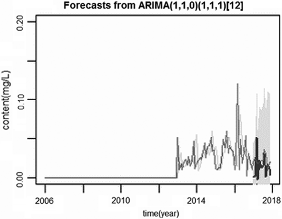
Comparison of TP sample data and forecast data.

FIG. 9.

Comparison of TN Sample Data With Forecast Data.

Predictive value of TP and TN

According to Table 1, from the prediction effect of TP, the highest accuracy was 96%, the lowest was 82%, and the final average prediction error was 9.6%. Judging from the data law of error, the accuracy of prediction was gradually increased with the increase of the month. We can use this feature to improve the accuracy of prediction. Compared (Dai et al., 2017) with the predicted value of TN, the average error of TP was larger. Combined with practical investigation and consulting a large number of documents, the team found that the sample container was absolutely clean and best to be analyzed immediately after the absorption of phosphate. If not, the content of TP in the water would be affected, and the water sample would be dissolved. There may be a certain artificial error in the TP content.

Table 1.

Total Phosphorus Forecast from January to July 2017

Month	Actual data (mg/L)	Predictive value (mg/L)
1	0.021	0.018
2	0.0243	0.02
3	0.018	0.016
4	0.017	0.016
5	0.02	0.019
6	0.0218	0.021

According to Table 2, from the perspective of the prediction effect of TN, the prediction accuracy was up to 99%, the lowest was 95%, and the final average prediction error was 2.5%. It can be seen that the prediction results were in line with the actual situation, and the results were convincing. Compared with the prediction effect of TP, the TN error was smaller. Although the TN measurement process was also affected by many factors, the measurement error was small in view of the more effective methods of controlling the control error.

Table 2.

Total Nitrogen Forecast from January to July 2017

Month	Actual data (mg/L)	Predictive value (mg/L)
1	5.49	5.56
2	5.87	5.96
3	5.98	6.13
4	6.44	6.12
5	6.32	5.98
6	5.19	5.23
7	3.98	3.96

Compared with the conclusion (Ding et al., 2014) obtained by other methods, this method was closer to the reality. Considering that the water quality was influenced by factors such as season and climate, a small amount of data that were closest to the future was used to predict accurately, and the purpose of real-time monitoring was achieved. In addition, the water quality prediction was closely connected with the accuracy of historical data, and the data source of this team was scientific and reliable, which lays a solid foundation for the success of data processing. As the most important influencing factor of water pollution, the accurate prediction of phosphorus and nitrogen in water quality was of great significance, and it can effectively improve the living environment of humans in time.

After the prediction of phosphorus and nitrogen contents in the Shihe reservoir is completed by the method just cited, we further study the degree of eutrophication of the water body and make timely protective measures. According to the simple indicator that the nitrogen content in the water is more than 0.3 mg/L and the phosphorus content is more than 0.01 mg/L, it means that the eutrophication of the water is more serious and needs to be treated. We can achieve the purpose of water quality monitoring and early warning, so as to manage the water quality of the reservoir with low cost and high quality. At this time, appropriate measures should be taken, such as the proper breeding of herbivorous fish, the planting of aquatic higher plants, etc. Through the environment-friendly biotechnology, the purpose of harmonious development of nature and humanity is achieved.

Conclusion

This study uses environmental surveys and water quality monitoring to determine the load of nitrogen and phosphorus pollution in the reservoir and establish an ARIMA model based on time series. With the optimization of the Holt-Winters seasonal model, the prediction accuracy is as high as 97.5%, and the prediction data and the sample data have a good fitting effect and are superior to most of the prediction models. For seasonally significant data, using the Holt-Winters seasonal model can accurately reflect the hidden patterns between data and facilitate multidimensional analysis of data. In addition, the method adopted in this article improves the shortcoming of the neural network model, that is, the larger the amount of data, the better the prediction effect, making the idea of “small data accurately predicting the future” become a reality. Through the prediction and analysis of the TP and TN of the Shihe reservoir, the degree of eutrophication can be obtained indirectly, and it can achieve the purpose of simplifying the detection and prevention of water pollution. It is of great significance to strengthen the management of reservoir water quality, especially the construction of new reservoirs.

Taking the Shihe reservoir for example, this article establishes a water quality change trend model based on nitrogen and phosphorus nutrients in the reservoir, and it quantifies the relationship between time and nitrogen and phosphorus concentrations. Combined with the model prediction results and the comprehensive characteristics of the water environment, the prediction model established in this article can be applied to different water quality situations through its independent correction control ability. Under the premise of ensuring the accuracy of prediction, the existing general methods are optimized so that the managers of reservoirs can monitor the degree of eutrophication of the reservoir through the nitrogen and phosphorus content and provide corresponding data support for the control and treatment of water pollution. This model has simplified the detection step of the eutrophication of the reservoir, reduced the cost of water quality monitoring, and improved the efficiency of water environmental protection.

Footnotes

Acknowledgments

This work was supported by colleges and universities in Hebei Province science and technology research project (Education Science Research Program of Hebei Provincial Department Z2012068), independent research program of young teachers in Yanshan University 14LGA018, the National Natural Science Foundation of China 21476190, research project on social science development in Hebei Province in 2017 (201705120102), and 2016 Hebei Province humanities and social sciences research project (GH161008).

Author Disclosure Statement

No competing financial interests exist.

References

Abdelmalik

K.W.

(2016). Role of statistical remote sensing for Inland water quality parameters prediction. Egypt. J. Remote Sensing Space Sci. 21, 154.

Avila

, Horn

, Moriarty

, Hodson

, and Moltchanova

(2018). Evaluating statistical model performance in water quality prediction. J. Environ. Manage. 206, 910.

Bedri

, Corkery

, O'Sullivan

J.J.

, Deering

L.A.

, and Demeter

(2016). Evaluating a microbial water quality prediction model for beach management under the revised EU Bathing Water Directive. J. Environ. Manage. 167, 49.

Chou

J.S.

, Ho

C.C.

, and Hoang

H.S.

(2018). Determining quality of water in reservoir using machine learning. Ecol. Inform. 44, 57.

Dai

Q.S.

, Wang

P.F.

, Wang

, Yu

, Liu

J.J.

, and Jun

(2017). Prediction and analysis of the water quality of the two river sluice section of Hongze Lake drinking water source based on the LWCA-SVM model. China Rural Water Conservancy Hydropower. 07, 62.

Ding

Y.R.

, Cai

Y.G.

, Sun

P.D.

, and Chen

(2014). The use of combined neural networks and genetic algorithms for prediction of river water quality. J. Appl. Res. Technol. 12, 493.

Guo

X.C.

, Du

P.F.

, Zhao

D.Q.

, and Ma

H.T.

(2018). Optimization of Pingshui River water quality monitoring point. China Environ. Monit. 01, 1.

Jaddi

N.S.

, and Abdullah

(2017). Acooperative-competitive master-slave global-best harmony search for ANN optimization and water-quality prediction. Appl. Soft Comput. 51, 209.

Khadr

, and Elshemy

(2016). Data-driven modeling for water quality prediction case study: The drains system associated with Manzala Lake, Egypt. Ain Shams Eng. J. 8, 549.

10.

Lavrenz

S.M.

, Vlahogianni

E.I.

, Gkritza

, and Ke

(2018). Time series modeling in traffic safety research. Accid. Anal. Prev. 117, 368.

11.

Liu

, Wang

, Zhou

, and Jiang

(2018). Appropriate use of the increment entropy for electrophysiological time series. Comput. Biol. Med. 95, 13.

12.

Liu

, Long

, Zhao

J.D.

, and Du

Q.Z.

(2017). Water quality prediction of PCA River by GABP technology. J. Yunnan Univ. (Nat. Sci.). 01, 39.

13.

Mikalsen

K.Ø.

, Bianchi

F.M.

, Sogueroruiz

, and Jenssen

(2018). Time series cluster kernel for learning similarities between multivariate time series with missing data. Pattern Recognit. 76, 569.

14.

Orzepowski

, Paruch

A.M.

, Pulikowski

, et al. (2014). Quantitative and qualitative assessment of agricultural water resources under variable climatic conditions of Silesian Lowlands (Southwest Poland). Agric. Water Manage. 138, 45.

15.

Rizo-Decelis

L.D.

, Pardo-Igúzquiza

, and Andreo

(2017). Spatial prediction of water quality variables along a main river channel, in presence of pollution hotspots. Sci. Total Environ. 605, 276.

16.

State Environmental Protection Administration (SEPA). (2002). Environment Quality Standards for Surface Water.

17.

Wang

, Engel

BA.

, Huang

, Peng

, and Zhang

(2018). Accurately early warning to water quality pollutant risk by mobile model system with optimization technology. J. Environ. Manage. 208, 122.

18.

, Zhou

, Sun

, and Du

(2016). Water temperature and pH prediction model of aquaculture based on particle swarm optimization BP neural network. Fishery Modernization. 01, 24.

19.

Zhang

, Wei

, Tang

, Feng

, and Wu

D.-C.

(2016). A prediction model for the COD detection of water quality by UV visible spectrum method. Laser Mag. 04, 21.

20.

Zhang

, Zhang

, Wen

, Zhang

, and Yuan

(2018). Discriminative extraction of features from time series. Neurocomputing. 275, 2317.