Application of Mixed-Integer Nonlinear Optimization Programming Based on Ensemble Surrogate Model for Dense Nonaqueous Phase Liquid Source Identification in Groundwater

Abstract

Groundwater contamination source identification (GCSI) is critical for taking effective measures to protect groundwater resources, assess risks, mitigate disasters, and design remediation strategies. Simulation–optimization techniques have been effective tools for GCSI. However, previous studies have applied individual surrogate models when replacing simulation models, rather than making efforts to combine various methods to improve the approximation accuracy of the surrogate model over the simulation model. In this study, the kernel extreme learning machine (KELM) model was proposed to enhance the surrogate model, and to approach GCSI problems, especially those of dense nonaqueous phase liquid-contaminated aquifers, more effectively. In addition, a kriging model and a support vector regression (SVR) model were built and compared with the KELM model, and various ensemble surrogate (ES) modeling techniques were applied to establish four ES models. Results showed that the KELM model was more accurate than the kriging and SVR models; however, the ES models performed much better than the three individual surrogate models. The most precise ES model increased the certainty coefficient (R²) to 0.9837, whereas limiting the maximum relative error to 13.14%. Finally, a mixed-integer nonlinear programming optimization model was established to identify the groundwater contamination source in terms of location and release history, and simultaneously assess aquifer parameters. The ES model developed in this article could reasonably predict the system response under given operation conditions. Replacement of the simulation model by the ES model considerably reduced the computation burden of the simulation–optimization process and simultaneously achieved high computation accuracy.

Introduction

Groundwater contamination source identification (GCSI), including number, location, and release history (Atmadja and Bagtzoglou, 2001; Sun et al., 2006; Sun, 2009), is critical for taking effective measures to protect groundwater resources, assess risks, mitigate disasters, and design remediation strategies (Mirghani et al., 2012; Om and Bithin, 2013).

Comprehensive reviews of GCSI studies have been provided by several researchers (Michalak and Kitanidis, 2004; Bagtzoglou and Atmadja, 2005), suggesting that the simulation–optimization method was the most widely applied approach (e.g., Ayvaz and Karahan, 2008; Mirghani et al., 2009; Ayvaz, 2010; Datta et al., 2011). However, GCSI studies at dense nonaqueous phase liquid (DNAPL)-contaminated sites are rare. Sciortino et al. (2000) formulated inverse modeling for locating DNAPL pools in groundwater as a least squares minimization problem, solved by a search procedure based on the Levenberg–Marquardt method. Gzyl et al. (2014) performed integral pumping tests to identify the locations of DNAPL sources in southern Poland and applied a geostatistical approach to identify their release history.

Any GCSI approach should be based on a simulation model, which simulates flow and contaminant transport processes in the aquifer. A reliable quantification of aquifer parameters (hydraulic conductivity, porosity, dispersivity, etc.) is essential as this determines the quality of the simulation model prediction. However, in many real-life situations, either all or some of the aquifer parameters are unknown, and calibration and verification of the simulation model cannot be carried out without knowing the contamination source. A reliable estimation of the aquifer flow and transport parameters is a prerequisite for accurately identifying an unknown contamination source.

Only a few studies (Mahar and Datta, 2001; Datta et al., 2009) have attempted to solve the problems of GCSI and aquifer parameters simultaneously, which makes the GCSI challenge more complex. To enhance the reliability of such multiparameter studies and achieve more realistic research results, we presented a mixed-integer nonlinear optimization approach to identify groundwater contamination sources in terms of location and release history, and simultaneously assess the aquifer parameters at DNAPL-contaminated sites. In addition, an ensemble surrogate (ES) model, replacing the multiphase flow simulation model, was coupled with the mixed-integer nonlinear programming model to reduce the high computational burden that resulted from incorporating the simulation model repeatedly in the optimization process.

The surrogate model is an approximation model with an input and output relationship similar to the simulation model, but needing far less run time (Queipo et al., 2005; Sreekanth and Datta, 2010; Hou et al., 2017). The computational burden is significantly reduced by replacing the numerical simulation model with a more efficient surrogate model. The most crucial objective was to improve the approximation accuracy of the surrogate model, which has a great impact on the reliability of the simulation–optimization process.

The artificial neural network method is most widely used as a surrogate model for numerical simulation of GCSI (Singh et al., 2004; Mirghani et al., 2012; Srivastava and Singh, 2014, 2015). However, it suffers from instability and overfitting problems that are difficult to solve. The kriging model was tested on several occasions (Zhao et al., 2016) to solve GCSI problems; however, its suitability in terms of identifying DNAPL-contaminated aquifers has not been tested before. There are only a few other surrogate models in place that try to solve GCSI problems.

This study proposed three surrogate models: kernel extreme learning machine (KELM) model, support vector regression (SVR) model, and kriging model to solve GCSI problems at DNAPL-contaminated site. Furthermore, different surrogate modeling methods were combined to enhance the capabilities of the individual surrogate models. A comparative study was conducted to find the best ES modeling technique.

ES modeling techniques have been developed for just a few years. Sreekanth and Datta (2011) presented an ES-based simulation–optimization approach for coastal aquifer management strategies. The ES model was built on several genetic programming models, trained by different realizations of one training sample data set obtained by nonparametric bootstrapping. Müller and Shoemaker (2014) examined various surrogate models, sampling strategies, and combinations of surrogate models (ES models) for optimization of computationally expensive remediation strategies. Jiang et al. (2015) combined the kriging and KELM models to establish an ES model for optimizing the strategy of surfactant-enhanced aquifer remediation. However, these ES models were all related to aquifer management strategies or optimization of remediation strategies. The ES modeling technique has not been applied to GCSI problems.

The main contribution of this study is to develop and enrich the technical implications for identifying the source of DNAPL-contaminated aquifers. The novelties of this article are as follows: (1) Different ES models, incorporating the kriging, SVR, and KELM methods, were proposed and compared for their suitability of GCSI. (2) A mixed-integer nonlinear programming approach was presented to identify groundwater contamination sources in terms of location and release history, and simultaneously estimate aquifer parameters at DNAPL-contaminated sites.

Methodology

Multiphase flow numerical simulation model

Any meaningful approach to GCSI problems must obey the flow and transport principle. Thus, the simulation model, which reconstructs transportation and transformation of contaminants in the aquifer, is set as an equality constraint in the simulation–optimization method (Datta et al., 2011). The process of the simulation-surrogate-optimization method in this article is shown in Figure 1.

FIG. 1.

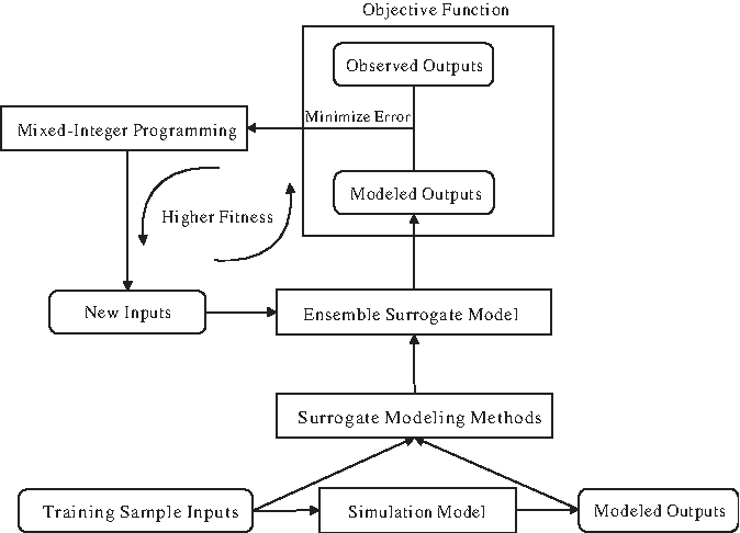
Flowchart of proposed groundwater contamination source identification solution process.

The basic mass conservation equation for each component of multiphase flow can be written as follows (Lu et al., 2013; Hou et al., 2015; Jiang et al., 2015): \documentclass{aastex}\usepackage{amsbsy}\usepackage{amsfonts}\usepackage{amssymb}\usepackage{bm}\usepackage{mathrsfs}\usepackage{pifont}\usepackage{stmaryrd}\usepackage{textcomp}\usepackage{portland, xspace}\usepackage{amsmath, amsxtra}\usepackage{upgreek}\pagestyle{empty}\DeclareMathSizes{10}{9}{7}{6}\begin{document} \[\frac{{\partial \left( {\phi {{\tilde C}_k}{\rho _k}} \right)}}{{\partial t}} + \vec \nabla \left[ {\sum\limits_{l = 1}^2 {{\rho _k}({C_{kl}}{{\vec v}_l} - \phi {S_l}{{\mathop {\mathop K\limits^ \to }\limits^ \to}_{kl}} \vec \nabla {C_{kl}})} } \right] = {R_k},{\text{ }} \tag{1} \] \end{document}

where k is component index, l is phase index, including water and oil, ø is porosity, \documentclass{aastex}\usepackage{amsbsy}\usepackage{amsfonts}\usepackage{amssymb}\usepackage{bm}\usepackage{mathrsfs}\usepackage{pifont}\usepackage{stmaryrd}\usepackage{textcomp}\usepackage{portland, xspace}\usepackage{amsmath, amsxtra}\usepackage{upgreek}\pagestyle{empty}\DeclareMathSizes{10}{9}{7}{6}\begin{document} $$ { \tilde C_k} $$ \end{document} is overall concentration by volume fraction of component k, ρ_k is density of component k (kg/m³), C_kl is concentration by volume fraction of component k in phase l, \documentclass{aastex}\usepackage{amsbsy}\usepackage{amsfonts}\usepackage{amssymb}\usepackage{bm}\usepackage{mathrsfs}\usepackage{pifont}\usepackage{stmaryrd}\usepackage{textcomp}\usepackage{portland, xspace}\usepackage{amsmath, amsxtra}\usepackage{upgreek}\pagestyle{empty}\DeclareMathSizes{10}{9}{7}{6}\begin{document} $$ { \vec v_l} $$ \end{document} is Darcy velocity of phase l (m/s), S_l is saturation of phase l, is dispersion tensor (m²/s), and R_k is total sources and sinks of component k (kg/[m³·s]). Initial and boundary conditions were integrated in the mass conservation equation to build the mathematical model; in this article the mathematical model was solved by UTCHEM (University of Texas Chemical Compositional Simulator).

KELM method

Kriging method, SVR method, and KELM method were applied to building the surrogate models of multiphase flow simulation model. The detailed introduction of kriging method and SVR method can be found in Hou et al. (2015, 2016), and the detailed introduction of KELM method is as follows.

KELM was used to generalize extreme learning machine (ELM) by transforming the explicit activation function to an implicit mapping function (Chen et al., 2014; Shi et al., 2014; Hou and Lu, 2018a).

For training sample \documentclass{aastex}\usepackage{amsbsy}\usepackage{amsfonts}\usepackage{amssymb}\usepackage{bm}\usepackage{mathrsfs}\usepackage{pifont}\usepackage{stmaryrd}\usepackage{textcomp}\usepackage{portland, xspace}\usepackage{amsmath, amsxtra}\usepackage{upgreek}\pagestyle{empty}\DeclareMathSizes{10}{9}{7}{6}\begin{document} $$ ( {{ \bf{x}}_j} , {t_j} ) , j = 1 , \ldots , N $$ \end{document} . The output y_j of ELM is \documentclass{aastex}\usepackage{amsbsy}\usepackage{amsfonts}\usepackage{amssymb}\usepackage{bm}\usepackage{mathrsfs}\usepackage{pifont}\usepackage{stmaryrd}\usepackage{textcomp}\usepackage{portland, xspace}\usepackage{amsmath, amsxtra}\usepackage{upgreek}\pagestyle{empty}\DeclareMathSizes{10}{9}{7}{6}\begin{document} \begin{align*} \mathop \sum \limits_{i = 1}^L {{ \beta _i} \cdot } p ( { \omega _i}{{ \bf{x}}_j} + {b_i} ) = { \bf{q ( }}{{ \bf{x}}_j}{{ \bf{ ) }}^{ \bf{T}}} \cdot { { \beta }} = f ( {{ \bf{x}}_j} ) { \rm{ = }}{y_j} , \tag{2} \end{align*} \end{document} \documentclass{aastex}\usepackage{amsbsy}\usepackage{amsfonts}\usepackage{amssymb}\usepackage{bm}\usepackage{mathrsfs}\usepackage{pifont}\usepackage{stmaryrd}\usepackage{textcomp}\usepackage{portland, xspace}\usepackage{amsmath, amsxtra}\usepackage{upgreek}\pagestyle{empty}\DeclareMathSizes{10}{9}{7}{6}\begin{document} \begin{align*} { \bf{q ( }}{{ \bf{x}}_j}{ \bf{ ) }} = { \left[ {p ( { \omega _1}{{ \bf{x}}_j} + {b_1} ) , p ( { \omega _2}{{ \bf{x}}_j} + {b_2} ) , \ldots , p ( { \omega _L}{{ \bf{x}}_j} + {b_L} ) } \right] ^{ \bf{T}}} , \tag{3} \end{align*} \end{document}

\documentclass{aastex}\usepackage{amsbsy}\usepackage{amsfonts}\usepackage{amssymb}\usepackage{bm}\usepackage{mathrsfs}\usepackage{pifont}\usepackage{stmaryrd}\usepackage{textcomp}\usepackage{portland, xspace}\usepackage{amsmath, amsxtra}\usepackage{upgreek}\pagestyle{empty}\DeclareMathSizes{10}{9}{7}{6}\begin{document} $$ p ( \cdot ) $$ \end{document} is the activation function, input nodes connect to the ith hidden neuron, \documentclass{aastex}\usepackage{amsbsy}\usepackage{amsfonts}\usepackage{amssymb}\usepackage{bm}\usepackage{mathrsfs}\usepackage{pifont}\usepackage{stmaryrd}\usepackage{textcomp}\usepackage{portland, xspace}\usepackage{amsmath, amsxtra}\usepackage{upgreek}\pagestyle{empty}\DeclareMathSizes{10}{9}{7}{6}\begin{document} $$ i = 1 , \ldots , L $$ \end{document} , through the weight vector ω_i, and b_i is the threshold. Thus, \documentclass{aastex}\usepackage{amsbsy}\usepackage{amsfonts}\usepackage{amssymb}\usepackage{bm}\usepackage{mathrsfs}\usepackage{pifont}\usepackage{stmaryrd}\usepackage{textcomp}\usepackage{portland, xspace}\usepackage{amsmath, amsxtra}\usepackage{upgreek}\pagestyle{empty}\DeclareMathSizes{10}{9}{7}{6}\begin{document} $$ p ( { \omega _i}{{ \bf{x}}_j} + {b_i} ) $$ \end{document} is the output function of the ith hidden neuron, and ith the hidden neuron connected to the output neuron through the weight β_i (Jiang et al., 2015).

Equation (2) is expressed in the matrix–vector form as \documentclass{aastex}\usepackage{amsbsy}\usepackage{amsfonts}\usepackage{amssymb}\usepackage{bm}\usepackage{mathrsfs}\usepackage{pifont}\usepackage{stmaryrd}\usepackage{textcomp}\usepackage{portland, xspace}\usepackage{amsmath, amsxtra}\usepackage{upgreek}\pagestyle{empty}\DeclareMathSizes{10}{9}{7}{6}\begin{document} \begin{align*} { \bf{Q \beta }} = { \bf{Y}} , \tag{4} \end{align*} \end{document}

\documentclass{aastex}\usepackage{amsbsy}\usepackage{amsfonts}\usepackage{amssymb}\usepackage{bm}\usepackage{mathrsfs}\usepackage{pifont}\usepackage{stmaryrd}\usepackage{textcomp}\usepackage{portland, xspace}\usepackage{amsmath, amsxtra}\usepackage{upgreek}\pagestyle{empty}\DeclareMathSizes{10}{9}{7}{6}\begin{document} $$ { { \beta }} = { [ { \beta _1} , \ldots , { \beta _L} ] ^T} $$ \end{document} , \documentclass{aastex}\usepackage{amsbsy}\usepackage{amsfonts}\usepackage{amssymb}\usepackage{bm}\usepackage{mathrsfs}\usepackage{pifont}\usepackage{stmaryrd}\usepackage{textcomp}\usepackage{portland, xspace}\usepackage{amsmath, amsxtra}\usepackage{upgreek}\pagestyle{empty}\DeclareMathSizes{10}{9}{7}{6}\begin{document} $$ { \bf{Y}} = { [ {y_1} , \ldots , {y_N} ] ^T} $$ \end{document} and Q is the hidden layer output matrix of ELM: \documentclass{aastex}\usepackage{amsbsy}\usepackage{amsfonts}\usepackage{amssymb}\usepackage{bm}\usepackage{mathrsfs}\usepackage{pifont}\usepackage{stmaryrd}\usepackage{textcomp}\usepackage{portland, xspace}\usepackage{amsmath, amsxtra}\usepackage{upgreek}\pagestyle{empty}\DeclareMathSizes{10}{9}{7}{6}\begin{document} \[{\mathbf{Q}} = {\text{ }}{\left[ {\begin{array}{*{20}{c}} {p({\omega _1}{{\mathbf{x}}_1} + {b_1}) \cdots p({\omega _L}{{\mathbf{x}}_1} + {b_L})} \\ {\;\;\;\;\;\;\;\;\; \vdots \;\;\;\;\;\;\;\;\;{\mkern 1mu} \ddots \;\;\;\;\;\;\;\;\;\;\;\;\; \vdots {\text{ }}} \\ {p({\omega _i}{{\mathbf{x}}_N} + {b_i}){\mkern 1mu} \cdots p({\omega _L}{{\mathbf{x}}_N} + {b_L})} \end{array}} \right]_{N \times L.}} \tag{5} \] \end{document}

If the ELM model with L hidden nodes can learn these N training samples with no residuals, then Equation (2) exists (Wang and Han, 2014): \documentclass{aastex}\usepackage{amsbsy}\usepackage{amsfonts}\usepackage{amssymb}\usepackage{bm}\usepackage{mathrsfs}\usepackage{pifont}\usepackage{stmaryrd}\usepackage{textcomp}\usepackage{portland, xspace}\usepackage{amsmath, amsxtra}\usepackage{upgreek}\pagestyle{empty}\DeclareMathSizes{10}{9}{7}{6}\begin{document} \begin{align*} \mathop \sum \limits_{i = 1}^L {{ \beta _i} \cdot } p ( { \omega _i}{{ \bf{x}}_j} + {b_i} ) = { \bf{q ( }}{{ \bf{x}}_j}{{ \bf{ ) }}^{ \bf{T}}} \cdot { { \beta }} = f ( {{ \bf{x}}_j} ) = {t_j} \quad j = 1 , \ldots , N , \tag{6} \end{align*} \end{document}

where t_j denotes the target value.

Equation (6) can be written compactly as \documentclass{aastex}\usepackage{amsbsy}\usepackage{amsfonts}\usepackage{amssymb}\usepackage{bm}\usepackage{mathrsfs}\usepackage{pifont}\usepackage{stmaryrd}\usepackage{textcomp}\usepackage{portland, xspace}\usepackage{amsmath, amsxtra}\usepackage{upgreek}\pagestyle{empty}\DeclareMathSizes{10}{9}{7}{6}\begin{document} \begin{align*} { \bf{Q \beta }} = { \bf{T}}. \tag{7} \end{align*} \end{document}

The smallest norm least-squares solution of Equation (7) is defined as \documentclass{aastex}\usepackage{amsbsy}\usepackage{amsfonts}\usepackage{amssymb}\usepackage{bm}\usepackage{mathrsfs}\usepackage{pifont}\usepackage{stmaryrd}\usepackage{textcomp}\usepackage{portland, xspace}\usepackage{amsmath, amsxtra}\usepackage{upgreek}\pagestyle{empty}\DeclareMathSizes{10}{9}{7}{6}\begin{document} \begin{align*} {{ \beta }} = {{ \bf{Q}}^{ \bf{ + }}}{ \bf{T}} , \tag{8} \end{align*} \end{document}

\documentclass{aastex}\usepackage{amsbsy}\usepackage{amsfonts}\usepackage{amssymb}\usepackage{bm}\usepackage{mathrsfs}\usepackage{pifont}\usepackage{stmaryrd}\usepackage{textcomp}\usepackage{portland, xspace}\usepackage{amsmath, amsxtra}\usepackage{upgreek}\pagestyle{empty}\DeclareMathSizes{10}{9}{7}{6}\begin{document} $$ {{ \bf{Q}}^{ \bf{ + }}} $$ \end{document} is the Moore–Penrose generalized inverse of \documentclass{aastex}\usepackage{amsbsy}\usepackage{amsfonts}\usepackage{amssymb}\usepackage{bm}\usepackage{mathrsfs}\usepackage{pifont}\usepackage{stmaryrd}\usepackage{textcomp}\usepackage{portland, xspace}\usepackage{amsmath, amsxtra}\usepackage{upgreek}\pagestyle{empty}\DeclareMathSizes{10}{9}{7}{6}\begin{document} $$ { \bf{Q}} $$ \end{document} : \documentclass{aastex}\usepackage{amsbsy}\usepackage{amsfonts}\usepackage{amssymb}\usepackage{bm}\usepackage{mathrsfs}\usepackage{pifont}\usepackage{stmaryrd}\usepackage{textcomp}\usepackage{portland, xspace}\usepackage{amsmath, amsxtra}\usepackage{upgreek}\pagestyle{empty}\DeclareMathSizes{10}{9}{7}{6}\begin{document} \begin{align*} {{ \bf{Q}}^{ \bf{ + }}} = {{ \bf{Q}}^{ \bf{T}}}{ ( { \bf{Q}}{{ \bf{Q}}^{ \bf{T}}} ) ^{ - 1}}. \tag{9} \end{align*} \end{document}

Given N training samples \documentclass{aastex}\usepackage{amsbsy}\usepackage{amsfonts}\usepackage{amssymb}\usepackage{bm}\usepackage{mathrsfs}\usepackage{pifont}\usepackage{stmaryrd}\usepackage{textcomp}\usepackage{portland, xspace}\usepackage{amsmath, amsxtra}\usepackage{upgreek}\pagestyle{empty}\DeclareMathSizes{10}{9}{7}{6}\begin{document} $$ ( {{ \bf{x}}_j} , {t_j} ) ,\ j = 1 , \ldots , N $$ \end{document} , KELM is expressed as an optimization model: \documentclass{aastex}\usepackage{amsbsy}\usepackage{amsfonts}\usepackage{amssymb}\usepackage{bm}\usepackage{mathrsfs}\usepackage{pifont}\usepackage{stmaryrd}\usepackage{textcomp}\usepackage{portland, xspace}\usepackage{amsmath, amsxtra}\usepackage{upgreek}\pagestyle{empty}\DeclareMathSizes{10}{9}{7}{6}\begin{document} \[\begin{gathered} \min \;{L_P} = \frac{1}{2}{\left| \beta \right|^2} + \frac{C}{2}\sum\limits_{i = 1}^N {\xi _j^2} \hfill \\ s.t.\;\;\;{\mathbf{h}}{({{\mathbf{x}}_j})^{\mathbf{T}}} \cdot {\mathbf{\beta }} = {t_j} - {\xi _j}, \hfill \\ \end{gathered} \tag { 10 } \] \end{document}

β denotes a vector in the feature space F, C denotes the regularization coefficient, h(x_i) maps the input x_j to a vector in F, and ξ_j denotes the error (Wang and Han, 2014).

The optimization problem can be transformed into the Lagrange dual form \documentclass{aastex}\usepackage{amsbsy}\usepackage{amsfonts}\usepackage{amssymb}\usepackage{bm}\usepackage{mathrsfs}\usepackage{pifont}\usepackage{stmaryrd}\usepackage{textcomp}\usepackage{portland, xspace}\usepackage{amsmath, amsxtra}\usepackage{upgreek}\pagestyle{empty}\DeclareMathSizes{10}{9}{7}{6}\begin{document} \[{L_D} = \frac{1}{2}{\left| \beta \right|^2} + \frac{C}{2}\sum\limits_{j = 1}^N {\xi _j^2} - \sum\limits_{j = 1}^N {{\theta _j}} ({\mathbf{h}}{({{\mathbf{x}}_j})^{\mathbf{T}}} \cdot \beta - {t_j} + {\xi _j}), \tag { 11 } \] \end{document}

θ_i is the ith Lagrange multiplier. The problem can be computed by exploiting the Karush-Kuhn-Tucker (KKT) optimality conditions (Jiang et al., 2015).

The kernel matrix of ELM can be defined as \documentclass{aastex}\usepackage{amsbsy}\usepackage{amsfonts}\usepackage{amssymb}\usepackage{bm}\usepackage{mathrsfs}\usepackage{pifont}\usepackage{stmaryrd}\usepackage{textcomp}\usepackage{portland, xspace}\usepackage{amsmath, amsxtra}\usepackage{upgreek}\pagestyle{empty}\DeclareMathSizes{10}{9}{7}{6}\begin{document} \begin{align*} {{ \bf{K}}_{{ \bf{ELM}}}} = { \bf{Q}}{{ \bf{Q}}^{ \bf{T}}} , \tag{12} \end{align*} \end{document} \documentclass{aastex}\usepackage{amsbsy}\usepackage{amsfonts}\usepackage{amssymb}\usepackage{bm}\usepackage{mathrsfs}\usepackage{pifont}\usepackage{stmaryrd}\usepackage{textcomp}\usepackage{portland, xspace}\usepackage{amsmath, amsxtra}\usepackage{upgreek}\pagestyle{empty}\DeclareMathSizes{10}{9}{7}{6}\begin{document} \begin{align*} {K_{ELM ( i , j ) }} = { \bf{h ( }}{{ \bf{x}}_i}{{ \bf{ ) }}^{ \bf{T}}} \cdot { \bf{h ( }}{{ \bf{x}}_j}{ \bf{ ) }} = K ( {{ \bf{x}}_i} , {{ \bf{x}}_j} ) . \tag{13} \end{align*} \end{document}

Here, the radial basis function is usually applied as the kernel function \documentclass{aastex}\usepackage{amsbsy}\usepackage{amsfonts}\usepackage{amssymb}\usepackage{bm}\usepackage{mathrsfs}\usepackage{pifont}\usepackage{stmaryrd}\usepackage{textcomp}\usepackage{portland, xspace}\usepackage{amsmath, amsxtra}\usepackage{upgreek}\pagestyle{empty}\DeclareMathSizes{10}{9}{7}{6}\begin{document} $$ K ( {{ \bf{x}}_i} , {{ \bf{x}}_j} ) $$ \end{document} .

Finally, the KELM output function can be written as \documentclass{aastex}\usepackage{amsbsy}\usepackage{amsfonts}\usepackage{amssymb}\usepackage{bm}\usepackage{mathrsfs}\usepackage{pifont}\usepackage{stmaryrd}\usepackage{textcomp}\usepackage{portland, xspace}\usepackage{amsmath, amsxtra}\usepackage{upgreek}\pagestyle{empty}\DeclareMathSizes{10}{9}{7}{6}\begin{document} \[f({\mathbf{x}}) = {\mathbf{h}}{({\mathbf{x}})^{\mathbf{T}}}{{\mathbf{Q}}^{\mathbf{T}}}{\left( {{\mathbf{Q}}{{\mathbf{Q}}^{\mathbf{T}}} + \frac{{\mathbf{I}}}{C}} \right)^{ - 1}}{\mathbf{T}} = {\left[ {\begin{array}{*{20}{c}} {K({\mathbf{x}},{{\mathbf{x}}_1})} \\ {\; \vdots } \\ {K({\mathbf{x}},{{\mathbf{x}}_N})} \end{array}} \right]^T}\; \times {\left( {{{\mathbf{K}}_{{\mathbf{ELM}}}} + \frac{{\mathbf{I}}}{C}} \right)^{ - 1}}{\mathbf{T}}. \tag { 14 } \] \end{document}

ES models

Kriging model, SVR model, and KELM model were integrated to build the ES model. An ES model benefits from the predictability of each individual surrogate model, enhancing the overall prediction accuracy (Hou and Lu, 2018b). The individual surrogate models can be combined in two ways:

1. Build the kriging, SVR, and KELM models, respectively, using 90 training samples. The outputs of the ES model are the weighted sum of the outputs of the three models: \documentclass{aastex}\usepackage{amsbsy}\usepackage{amsfonts}\usepackage{amssymb}\usepackage{bm}\usepackage{mathrsfs}\usepackage{pifont}\usepackage{stmaryrd}\usepackage{textcomp}\usepackage{portland, xspace}\usepackage{amsmath, amsxtra}\usepackage{upgreek}\pagestyle{empty}\DeclareMathSizes{10}{9}{7}{6}\begin{document} \begin{align*} { \hat y_{ES}} ( { \bf{x}} ) = {w_1}{ \hat y_{KRG}} ( { \bf{x}} ) + {w_2}{ \hat y_{SVR}} ( { \bf{x}} ) + {w_3}{ \hat y_{KELM}} ( { \bf{x}} ) , \tag{15} \end{align*} \end{document}

where \documentclass{aastex}\usepackage{amsbsy}\usepackage{amsfonts}\usepackage{amssymb}\usepackage{bm}\usepackage{mathrsfs}\usepackage{pifont}\usepackage{stmaryrd}\usepackage{textcomp}\usepackage{portland, xspace}\usepackage{amsmath, amsxtra}\usepackage{upgreek}\pagestyle{empty}\DeclareMathSizes{10}{9}{7}{6}\begin{document} $$ { \hat y_{KRG}} ( { \bf{x}} ) $$ \end{document} , \documentclass{aastex}\usepackage{amsbsy}\usepackage{amsfonts}\usepackage{amssymb}\usepackage{bm}\usepackage{mathrsfs}\usepackage{pifont}\usepackage{stmaryrd}\usepackage{textcomp}\usepackage{portland, xspace}\usepackage{amsmath, amsxtra}\usepackage{upgreek}\pagestyle{empty}\DeclareMathSizes{10}{9}{7}{6}\begin{document} $$ { \hat y_{SVR}} ( { \bf{x}} ) $$ \end{document} , \documentclass{aastex}\usepackage{amsbsy}\usepackage{amsfonts}\usepackage{amssymb}\usepackage{bm}\usepackage{mathrsfs}\usepackage{pifont}\usepackage{stmaryrd}\usepackage{textcomp}\usepackage{portland, xspace}\usepackage{amsmath, amsxtra}\usepackage{upgreek}\pagestyle{empty}\DeclareMathSizes{10}{9}{7}{6}\begin{document} $$ { \hat y_{KELM}} ( { \bf{x}} ) $$ \end{document} is the response estimated by the kriging, SVR, and KELM models, and w₁, w₂, and w₃ are the weights for the surrogate models. The sum of the weights should equal 1.

2. Build four surrogate models using the best modeling method among kriging, SVR, and KELM with four training sample data sets. The outputs of the ES model are the weighted sum of the outputs of the four models. \documentclass{aastex}\usepackage{amsbsy}\usepackage{amsfonts}\usepackage{amssymb}\usepackage{bm}\usepackage{mathrsfs}\usepackage{pifont}\usepackage{stmaryrd}\usepackage{textcomp}\usepackage{portland, xspace}\usepackage{amsmath, amsxtra}\usepackage{upgreek}\pagestyle{empty}\DeclareMathSizes{10}{9}{7}{6}\begin{document} \begin{align*} { \hat y_{ES}} ( { \bf{x}} ) = \mathop \sum \limits_{i = 1}^4 {{w_i}{{ \hat y}_i} ( { \bf{x}} ) }. \tag{16} \end{align*} \end{document}

In addition, the weights of the individual surrogate models involved in the ES modeling can be calculated in two ways:

1. Weights are obtained using the root-mean-square error (RMSE) of the surrogate models: \documentclass{aastex}\usepackage{amsbsy}\usepackage{amsfonts}\usepackage{amssymb}\usepackage{bm}\usepackage{mathrsfs}\usepackage{pifont}\usepackage{stmaryrd}\usepackage{textcomp}\usepackage{portland, xspace}\usepackage{amsmath, amsxtra}\usepackage{upgreek}\pagestyle{empty}\DeclareMathSizes{10}{9}{7}{6}\begin{document} \[{w_i} = \frac{{1/{R_i}}}{{\sum\limits_{i = 1}^N {1/{R_i}} }},{\text{ }} \tag {17} \] \end{document}

where w_i is the weight for the ith surrogate model, R_i is the RMSE of the ith surrogate model obtained using testing samples, and N is the number of the surrogate models used for ES construction.

2. Optimal weights are obtained by solving an optimization problem of the form used in this work: \documentclass{aastex}\usepackage{amsbsy}\usepackage{amsfonts}\usepackage{amssymb}\usepackage{bm}\usepackage{mathrsfs}\usepackage{pifont}\usepackage{stmaryrd}\usepackage{textcomp}\usepackage{portland, xspace}\usepackage{amsmath, amsxtra}\usepackage{upgreek}\pagestyle{empty}\DeclareMathSizes{10}{9}{7}{6}\begin{document} \[\begin{gathered} {\text{minimize}}:\;RMSE\left[ {{{\hat y}_{ES}}({w_i})} \right] \hfill \\ = \sqrt {\frac{1}{M}\sum\limits_{k = 1}^M {{{\left[ {\sum\limits_{i = 1}^N {{w_i}{y_i} - {y_{actual}}} } \right]}^2}} } \hfill \\ {\text{subject}}\;{\text{to}}:\sum\limits_{i = 1}^N {{w_i}} {\text{ = 1}},{\text{ }} \hfill \\ \end{gathered} \tag {18} \] \end{document}

where y_i is the response estimated by the ith surrogate model, y_actual is the response estimated by the simulation model, and M is the number of testing samples.

0–1 mixed-integer nonlinear programming

The mathematical model established in the process of solving an optimization problem is the optimization model.

An optimization model generally consists of three elements: decision variables, objective functions, and constraints, and it can be expressed as \documentclass{aastex}\usepackage{amsbsy}\usepackage{amsfonts}\usepackage{amssymb}\usepackage{bm}\usepackage{mathrsfs}\usepackage{pifont}\usepackage{stmaryrd}\usepackage{textcomp}\usepackage{portland, xspace}\usepackage{amsmath, amsxtra}\usepackage{upgreek}\pagestyle{empty}\DeclareMathSizes{10}{9}{7}{6}\begin{document} \[\begin{gathered} \min \;f(X) \hfill \\ s.t.{\text{ }}\left\{ {_{{h_j}(X) = 0,j = 1,2, \ldots ,q,}^{{g_i}(X) \leqslant 0,i = 1,2, \ldots ,p}} \right. \hfill \\ \end{gathered} \tag{19} \] \end{document}

where \documentclass{aastex}\usepackage{amsbsy}\usepackage{amsfonts}\usepackage{amssymb}\usepackage{bm}\usepackage{mathrsfs}\usepackage{pifont}\usepackage{stmaryrd}\usepackage{textcomp}\usepackage{portland, xspace}\usepackage{amsmath, amsxtra}\usepackage{upgreek}\pagestyle{empty}\DeclareMathSizes{10}{9}{7}{6}\begin{document} $$ X{ \rm{ = ( }}{x_1} , {x_2}{ \rm{ , }} \ldots , {x_n}{{ \rm{ ) }}^T} $$ \end{document} is the decision variable vector, some of the variables are integer variables, whereas some are continuous variables, \documentclass{aastex}\usepackage{amsbsy}\usepackage{amsfonts}\usepackage{amssymb}\usepackage{bm}\usepackage{mathrsfs}\usepackage{pifont}\usepackage{stmaryrd}\usepackage{textcomp}\usepackage{portland, xspace}\usepackage{amsmath, amsxtra}\usepackage{upgreek}\pagestyle{empty}\DeclareMathSizes{10}{9}{7}{6}\begin{document} $$ f ( X ) $$ \end{document} is the objective function, \documentclass{aastex}\usepackage{amsbsy}\usepackage{amsfonts}\usepackage{amssymb}\usepackage{bm}\usepackage{mathrsfs}\usepackage{pifont}\usepackage{stmaryrd}\usepackage{textcomp}\usepackage{portland, xspace}\usepackage{amsmath, amsxtra}\usepackage{upgreek}\pagestyle{empty}\DeclareMathSizes{10}{9}{7}{6}\begin{document} $$ {g_i} ( X ) $$ \end{document} is the inequality constraint, and \documentclass{aastex}\usepackage{amsbsy}\usepackage{amsfonts}\usepackage{amssymb}\usepackage{bm}\usepackage{mathrsfs}\usepackage{pifont}\usepackage{stmaryrd}\usepackage{textcomp}\usepackage{portland, xspace}\usepackage{amsmath, amsxtra}\usepackage{upgreek}\pagestyle{empty}\DeclareMathSizes{10}{9}{7}{6}\begin{document} $$ {h_j} ( X ) $$ \end{document} is the equality constraint.

If some of the variables of the optimization model are integer variables and some are continuous variables, and if there are nonlinear objective functions or constraints, the optimization model is named mixed integer nonlinear programming. In addition, if the integer variables can only be 0 or 1, the optimization model is named 0–1 mixed integer nonlinear programming.

Case Study

Site overview

A hypothetical chlorobenzene-contaminated site was chosen as a case study to develop ES modeling techniques for GCSI problems in DNAPL-contaminated aquifers. A hypothetical case study was more suitable for the GCSI research, because the accuracy of GCSI results could be examined and the significance of the applied methodologies could be analyzed.

The investigation site was located in the saturated zone of a 20-m-deep phreatic aquifer with a complex mixture of clay and sand deposits in which the groundwater flowed in a right–left direction, and the horizontal hydraulic gradient was set to 0.0112. Our target was to identify the actual source among three potential contamination sources, and to analyze release strength, release duration, and, simultaneously, estimate aquifer parameters. Five observation wells were set at the lower reaches of the groundwater runoff to monitor the groundwater quality of the potential contamination sources (Fig. 2).

FIG. 2.

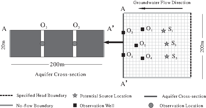
Schematic diagram of potential contamination sources, observation wells, and observation location.

Multiphase flow numerical simulation model

A three-dimensional multiphase flow numerical model was developed to simulate the transportation and transformation of contaminants in an aquifer with homogeneous conditions. Initial and boundary conditions were assumed to be known. The left and right boundaries of the site were set as first-type boundary conditions, and the phreatic surface was water exchange boundary, whereas the other boundaries were no-flux boundaries (Fig. 2). The simulation domain was discretized into 10 vertical layers and each layer was further discretized into 40 × 20 grids. Each grid measured is 10 × 10 × 2 m³.

The mathematical model of study area was built as follows: \documentclass{aastex}\usepackage{amsbsy}\usepackage{amsfonts}\usepackage{amssymb}\usepackage{bm}\usepackage{mathrsfs}\usepackage{pifont}\usepackage{stmaryrd}\usepackage{textcomp}\usepackage{portland, xspace}\usepackage{amsmath, amsxtra}\usepackage{upgreek}\pagestyle{empty}\DeclareMathSizes{10}{9}{7}{6}\begin{document} \begin{align*} \begin{split} & { \rm{Initial}} \;{ \rm{conditions :}} \\ & \left\{ \begin{matrix} { \left. {{P_l} \left( {x , y , z , t} \right) } \right\vert _{t = 0}} = P_l^0 \left( {x , y , z} \right) , \; \; \left( {x , y , z} \right) \in \Omega \hfill \\ { \left. {{S_l} \left( {x , y , z , t} \right) } \right\vert _{t = 0}} = S_l^0 \left( {x , y , z} \right) , \; \; \left( {x , y , z} \right) \in \Omega \hfill \\ { \left. {{C_{kl}} \left( {x , y , z , t} \right) } \right\vert _{t = 0}} = C_{kl}^0 \left( {x , y , z} \right) , \; \; \left( {x , y , z} \right) \in \Omega \hfill \\\end{matrix} \right. \\\end{split} \tag{21} \end{align*} \end{document} \documentclass{aastex}\usepackage{amsbsy}\usepackage{amsfonts}\usepackage{amssymb}\usepackage{bm}\usepackage{mathrsfs}\usepackage{pifont}\usepackage{stmaryrd}\usepackage{textcomp}\usepackage{portland, xspace}\usepackage{amsmath, amsxtra}\usepackage{upgreek}\pagestyle{empty}\DeclareMathSizes{10}{9}{7}{6}\begin{document} \begin{align*} \begin{split} & { \rm{Boundary \ conditions :}} \\ & \left\{ \begin{matrix} { \left. {{P_l} \left( {x , y , z , t} \right) } \right\vert _{{ \Gamma _1}}} = f_l^1 \left( {x , y , z , t} \right) , \; \; \left( {x , y , z} \right) \in { \Gamma _1} , \; \;t \ge 0 \hfill \\ { \left. {{{ \partial {P_l}} \over { \partial n}}} \right\vert _{{ \Gamma _2}}} = 0 , \; \; \left( {x , y , z} \right) \in { \Gamma _2} , \; \;t \ge 0 \hfill \\ { \left. {{C_{kl}}} \right\vert _{{ \Gamma _1}}} = \varphi _{kl}^1 \left( {x , y , z , t} \right) , \; \; \left( {x , y , z} \right) \in { \Gamma _1} , \; \;t \ge 0 \hfill \\ { \left. {{{ \partial {C_{kl}}} \over { \partial n}}} \right\vert _{{ \Gamma _2}}} = 0 , \; \; \left( {x , y , z} \right) \in { \Gamma _2} , \; \;t \ge 0 \hfill \\\end{matrix} \right. \\\end{split} \tag{22} \end{align*} \end{document}

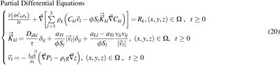
Here, part of the symbols in Equation (20) has been described in Equation (1). \documentclass{aastex}\usepackage{amsbsy}\usepackage{amsfonts}\usepackage{amssymb}\usepackage{bm}\usepackage{mathrsfs}\usepackage{pifont}\usepackage{stmaryrd}\usepackage{textcomp}\usepackage{portland, xspace}\usepackage{amsmath, amsxtra}\usepackage{upgreek}\pagestyle{empty}\DeclareMathSizes{10}{9}{7}{6}\begin{document} $$ {D_{dkl}} $$ \end{document} is the molecular diffusion coefficient of component k in phase l (m²/s), \documentclass{aastex}\usepackage{amsbsy}\usepackage{amsfonts}\usepackage{amssymb}\usepackage{bm}\usepackage{mathrsfs}\usepackage{pifont}\usepackage{stmaryrd}\usepackage{textcomp}\usepackage{portland, xspace}\usepackage{amsmath, amsxtra}\usepackage{upgreek}\pagestyle{empty}\DeclareMathSizes{10}{9}{7}{6}\begin{document} $$ \tau $$ \end{document} is the distortion coefficient, which should be >1, \documentclass{aastex}\usepackage{amsbsy}\usepackage{amsfonts}\usepackage{amssymb}\usepackage{bm}\usepackage{mathrsfs}\usepackage{pifont}\usepackage{stmaryrd}\usepackage{textcomp}\usepackage{portland, xspace}\usepackage{amsmath, amsxtra}\usepackage{upgreek}\pagestyle{empty}\DeclareMathSizes{10}{9}{7}{6}\begin{document} $$ { \delta _{ij}} $$ \end{document} is Kronecker \documentclass{aastex}\usepackage{amsbsy}\usepackage{amsfonts}\usepackage{amssymb}\usepackage{bm}\usepackage{mathrsfs}\usepackage{pifont}\usepackage{stmaryrd}\usepackage{textcomp}\usepackage{portland, xspace}\usepackage{amsmath, amsxtra}\usepackage{upgreek}\pagestyle{empty}\DeclareMathSizes{10}{9}{7}{6}\begin{document} $$ \delta $$ \end{document} function, a_Ll and a_Tl are the longitudinal dispersivity and transverse dispersivity (m), v_li and v_lj are the flow velocity components of phase l at direction i and direction j (m/s), k_rl is the relative permeability of phase l, is the intrinsic permeability (m²), \documentclass{aastex}\usepackage{amsbsy}\usepackage{amsfonts}\usepackage{amssymb}\usepackage{bm}\usepackage{mathrsfs}\usepackage{pifont}\usepackage{stmaryrd}\usepackage{textcomp}\usepackage{portland, xspace}\usepackage{amsmath, amsxtra}\usepackage{upgreek}\pagestyle{empty}\DeclareMathSizes{10}{9}{7}{6}\begin{document} $$ { \mu _l} $$ \end{document} is the viscosity of phase l (Pa/s), \documentclass{aastex}\usepackage{amsbsy}\usepackage{amsfonts}\usepackage{amssymb}\usepackage{bm}\usepackage{mathrsfs}\usepackage{pifont}\usepackage{stmaryrd}\usepackage{textcomp}\usepackage{portland, xspace}\usepackage{amsmath, amsxtra}\usepackage{upgreek}\pagestyle{empty}\DeclareMathSizes{10}{9}{7}{6}\begin{document} $$ { \rho _l} $$ \end{document} is the density of phase l, g is the acceleration of gravity (m/s²), z is the vertical distance (m), and P_l is the pressure of phase l (Pa).

Surrogate models of multiphase flow numerical simulation model

To identify the actual contamination source among three potential DNAPL sources, the release strengths and the release duration of three potential DNAPL sources and aquifer parameters were treated as controllable input variables to build the surrogate model. The input vectors of the surrogate model consist of eight elements: release strengths of S1, S2, S3, release durations, porosity, aqueous phase dispersivity, oleic phase dispersivity, and permeability.

As the objective function of the simulation–optimization model for GCSI was the minimal deviation between the actual observations and the model predictions, the size of the output of the surrogate model should match the actual groundwater quality observation data. Groundwater quality data were gathered in two sets with a time interval of 6 months. Each set of observation data included five constants, that is, the chlorobenzene concentrations in the middle part of the aquifer in each of the five observation wells (Fig. 2). Thus, the output vector of the surrogate model consists of 10 elements.

Four groups of training samples and 20 testing samples from potential regions of input were obtained using the Latin hypercube sampling (LHS) method; each training sample group consisted of 30 samples. The release strength and release duration were considered uniform distribution variables (0, 1.5 m³/day) and (600, 900 days). The aquifer parameters obey the normal distribution while LHS sampling, and the distribution characteristics of porosity, dispersivity, and permeability were taken as N (0.3, 0.0001), N (1 m, 0.01), and N (8,500 md, 100,000). The corresponding outputs of the 140 sets of input vectors were obtained for the developed simulation model runs. Four training sample groups were combined with each other to formulate four training sample data sets: groups 1–3, groups 1, 2, 4, groups 1, 3, 4, and groups 2–4. The kriging, SVR, and KELM models were built with the first training sample data set. Three individual surrogate models were then compared with each other using testing samples.

Undetermined parameters of each individual surrogate model were optimized by establishing a model using the minimal sum of the relative error by threefold cross-validation with 90 training samples as its objective function. The parameters served as decision variables and the constraints were the range of parameters. Genetic algorithm (GA) was used to solve the optimization models. The optimized parameters of three individual surrogate models are shown in Table 1.

Table 1.

Optimized Parameters of Individual Surrogate Models

Kriging	α₁	α₂	α₃	α₄	α₅	α₆	α₇	α₈
Value	0.0001	48.3427	2.1491	0.0016	1.9363	0.0002	53.1409	0.0013

SVR	Penalty factor C			Admitted deviation ɛ			Gaussian function parameter g
Value	8.7184			0.2015			0.0224

KELM	Regularization coefficient C			Kernel parameters γ (RBF)
Value	2043.1056			24.2838

KELM, kernel extreme learning machine; RBF, radial basis function; SVR, support vector regression.

Four ES models were established and compared in this article: (1) the ES model combining the kriging, SVR, and KELM models with the weights obtained using the RMSE of the surrogate models; (2) the ES model combining the kriging, SVR, and KELM models with the weights obtained using the optimization model; (3) the ES model combining four surrogate models using the best modeling method among kriging, SVR, and KELM models with four training sample data sets, and weights obtained using the RMSE of the surrogate models; (4) the ES model combining four surrogate models using the best modeling method among kriging, SVR, and KELM models with four training sample data sets, and weights obtained using the optimization model.

Surrogate model performance evaluation indexes

Three indexes were applied to evaluate the performance of the surrogate models: 1.

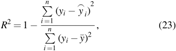
Certainty coefficient (R²)

where n is the sample number, y_i is the simulation model output, is the surrogate model output, and \documentclass{aastex}\usepackage{amsbsy}\usepackage{amsfonts}\usepackage{amssymb}\usepackage{bm}\usepackage{mathrsfs}\usepackage{pifont}\usepackage{stmaryrd}\usepackage{textcomp}\usepackage{portland, xspace}\usepackage{amsmath, amsxtra}\usepackage{upgreek}\pagestyle{empty}\DeclareMathSizes{10}{9}{7}{6}\begin{document} $$ {\overline {y}} $$ \end{document} is the average of the simulation model outputs. The surrogate model is more accurate when R² is closer to 1.

Mean relative error (MRE)

Maximum relative error

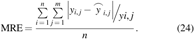
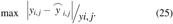
0–1 mixed-integer nonlinear programming optimization model

To identify the groundwater DNAPL contamination source, and simultaneously estimate the aquifer parameters, a 0–1 mixed integer nonlinear programming optimization model was established. The model was established by using the minimal deviation between actual observations and model predictions as objective function. Decision variables comprised source location, release strength, release duration, porosity, aqueous phase dispersivity, oleic phase dispersivity, and permeability.

The model was constrained by the range of decision variables, which were the same as the LHS potential regions. The surrogate model was embedded in the optimization model to replace the input/output relationship of the simulation model as follows:

Equation (26) shows the objective function and the constraints. \documentclass{aastex}\usepackage{amsbsy}\usepackage{amsfonts}\usepackage{amssymb}\usepackage{bm}\usepackage{mathrsfs}\usepackage{pifont}\usepackage{stmaryrd}\usepackage{textcomp}\usepackage{portland, xspace}\usepackage{amsmath, amsxtra}\usepackage{upgreek}\pagestyle{empty}\DeclareMathSizes{10}{9}{7}{6}\begin{document} $$ {C_k} ( t ) $$ \end{document} is the actual observation at the kth well, \documentclass{aastex}\usepackage{amsbsy}\usepackage{amsfonts}\usepackage{amssymb}\usepackage{bm}\usepackage{mathrsfs}\usepackage{pifont}\usepackage{stmaryrd}\usepackage{textcomp}\usepackage{portland, xspace}\usepackage{amsmath, amsxtra}\usepackage{upgreek}\pagestyle{empty}\DeclareMathSizes{10}{9}{7}{6}\begin{document} $$ k = 1 , \ldots , 5 $$ \end{document} , and \documentclass{aastex}\usepackage{amsbsy}\usepackage{amsfonts}\usepackage{amssymb}\usepackage{bm}\usepackage{mathrsfs}\usepackage{pifont}\usepackage{stmaryrd}\usepackage{textcomp}\usepackage{portland, xspace}\usepackage{amsmath, amsxtra}\usepackage{upgreek}\pagestyle{empty}\DeclareMathSizes{10}{9}{7}{6}\begin{document} $$ { \tilde C_k} ( t ) $$ \end{document} is the model prediction. \documentclass{aastex}\usepackage{amsbsy}\usepackage{amsfonts}\usepackage{amssymb}\usepackage{bm}\usepackage{mathrsfs}\usepackage{pifont}\usepackage{stmaryrd}\usepackage{textcomp}\usepackage{portland, xspace}\usepackage{amsmath, amsxtra}\usepackage{upgreek}\pagestyle{empty}\DeclareMathSizes{10}{9}{7}{6}\begin{document} $$ f ( { \bf{s}} , { \bf{p}} ) $$ \end{document} represents the ES model that transformed the source vector “s” and aquifer parameter vector “p” into concentrations C in the aquifer. The constraints present the lower and upper boundaries of the source release strength, source release duration, porosity, permeability, aqueous phase dispersivity, and oleic phase dispersivity in order. A GA was applied to solve the optimization model; the population size was set to 80 for the GA, and the algorithm was executed in 150 iterations.

Results and Discussion

Comparison of different individual surrogate models

Performance of three surrogate models were tested using 20 testing samples. Figure 3 shows the boxplots for the relative error metrics of the surrogate model outputs, each surrogate model containing 200 values. Given the maximum relative error and the distribution of the relative error values of the three surrogate models, we concluded that the approximation accuracy of the KELM and SVR models were acceptable. In addition, the approximation accuracy of the KELM model was slightly higher than that of the SVR model, whereas the approximation accuracy of the kriging model was unsatisfactory.

FIG. 3.

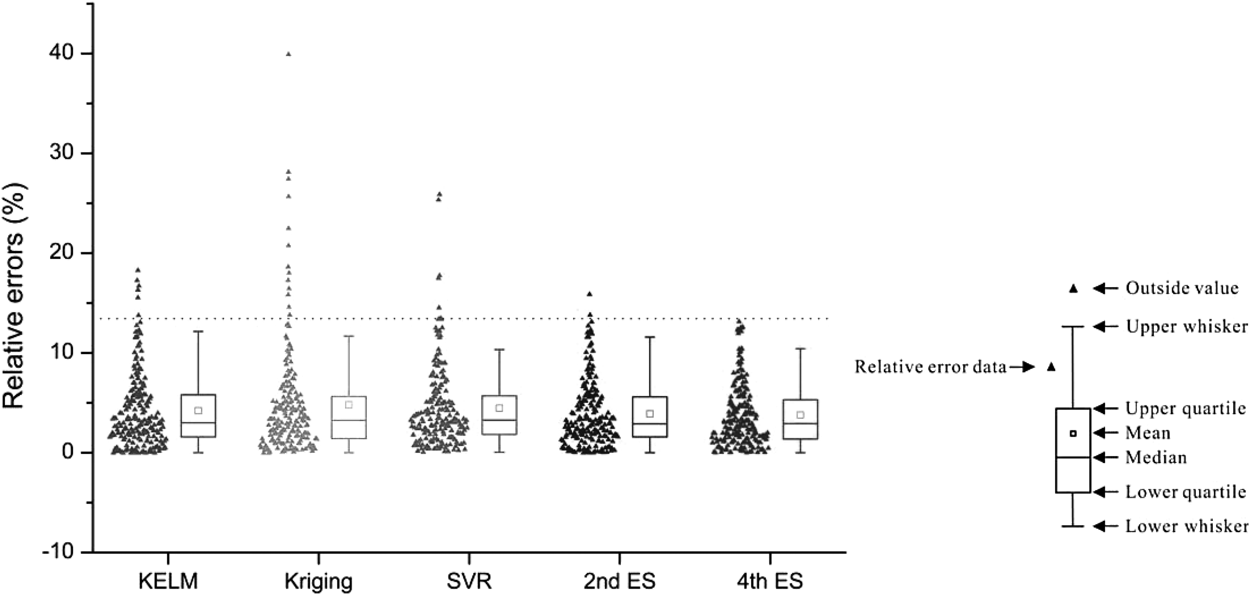
Boxplot of relative errors of ES models and three individual surrogate models. ES, ensemble surrogate; KELM, kernel extreme learning machine; SVR, support vector regression.

The same results were achieved by using the three aforementioned indexes to evaluate the three surrogate models (Table 2). The closer R² was to 1, the more accurate the surrogate model was. The KELM model was the most precise for all indexes (Bold values in Table 2).

Table 2.

Performance Evaluation of Surrogate Models

Performance evaluation indexes	Certainty coefficient R²	Mean relative error (%)	Maximum relative error (absolute value) (%)
Kriging	0.9719	5.18	39.90
SVR	0.9779	4.46	25.90
KELM	0.9793	4.21	18.26
KELM-120 training samples	0.9770	4.13	18.22
First ES model	0.9796	4.04	15.69
Second ES model	0.9805	3.90	15.87
Third ES model	0.9799	3.98	16.11
Fourth ES model	0.9837	3.77	13.14

ES, ensemble surrogate.

The transport of organic contaminants in a multiphase flow is complex, and the solubility of chlorobenzene in water is particularly small, which makes it hard to trace the relationship between input and output in a simulation model. The relative errors of the three surrogate models were higher than those of the same surrogate models when applied to other problems (Luo et al., 2013; Hou et al., 2015, 2016; Zhao et al., 2016). Thus, an ES model was required that further improved the approximation accuracy of the surrogate model and increased the reliability of GCSI data.

Comparison of ES models

Only the KELM and SVR models were used to build the ES models, as none of the other models delivered satisfactory approximation accuracy results. The presented ES models are (1) the first ES model, which combines SVR and KELM models with the weights obtained using the RMSE of the surrogate models; (2) the second ES model, which combines SVR and KELM models with the weights obtained using the optimization model; (3) the third ES model, which combines the four built surrogate models using KELM with four training sample data sets, and the weights obtained using the RMSE of the surrogate models; and (4) the fourth ES model, which combines the four built surrogate models using KELM with four training sample data sets; weights were obtained using the optimization model.

The outputs of the trained ES models, using 20 testing samples, were compared with the corresponding simulation model outputs. As an initial approach, the performance of the ES models was compared with those of the individual surrogate models. Figure 3 shows the boxplots for the relative error metrics of surrogate model outputs, and Figure 4 shows the relative error cumulative frequency curves of the surrogate models. Given the distribution of relative error data, we concluded that the second and the fourth ES models performed far better than the three individual surrogate models. Combining several KELM models built with different training sample data sets, and combining the surrogate models built by different methods, were effective ways to improve the reliability of the surrogate models.

FIG. 4.

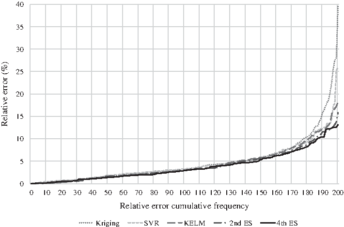
Relative error cumulative frequency curves of ES models and three individual surrogate models.

Four ES models were also compared with each other (Figs. 5 and 6). The fourth ES model performed better than the other three ES models. Building an optimization model to enhance the weights of the individual surrogate models involved in the ES modeling was necessary to improve the approximation accuracy. In addition, combining several KELM models built with different training sample data sets was more accurate than combining surrogate models built by different methods.

FIG. 5.

Boxplot of relative errors of ES models.

FIG. 6.

Relative error cumulative frequency curves of ES models.

The KELM model built with 120 training samples, that is, using all the training samples to build the third and fourth ES models, was part of the comparison; the relative error level of the KELM model was significantly higher than in the ES models (Fig. 6). From this it follows that an ES model is more reliable than an individual surrogate model, even when using the same surrogate modeling method and the same training sample data set.

The performance of the ES models using indexes are presented in Table 2. The fourth ES model delivered outstanding results with all indexes (Bold values in Table 2). The certainty coefficient (R²) of the fourth ES model increased to 0.9837, and the maximum relative error was only 13.14%, whereas the maximum relative errors of the other ES models were all >15%. It can be concluded that the fourth ES model is a reliable approach to replace the multiphase flow simulation model.

Comparison of mixed-integer optimization models

To fully exploit the advantage of the ES model, the fourth ES and the KELM models were each embedded in the optimization model, and the identification results were compared. The convergence of the objective function value during both identification processes are shown in Figure 7, and the identification results are compared in Table 3. Although the real location of the contamination source could be identified using both surrogate models, the identification results obtained by using the ES model were far better than those of the KELM model.

FIG. 7.

Convergence of objective function value during identification processes. (a) ES-based optimization model; (b) KELM-based optimization model.

Table 3.

Contamination Source Identification Results and Aquifer Parameters Estimation Results

Contamination source identification results	Source location	Release duration (days)	Release strength (m³/day)
Real value	S2	720	1.2000
ES-based identification results	S2	715	1.2353
Relative error (%)	0	0.6944	2.9435
KELM-based identification results	S2	701	1.2816
Relative error (%)	0	2.6389	6.8028

Aquifer parameters estimation results	Porosity	Permeability (md)	Aqueous phase dispersity (m)	Oleic phase dispersity (m)
Real value	0.3000	8,500	1.0000	1.0000
ES-based estimation results	0.2958	8,622	1.0367	1.0277
Relative error (%)	1.4067	1.4353	3.6723	2.7718
KELM-based estimation results	0.3176	8,297	1.0449	0.9374
Relative error (%)	5.8667	2.3882	4.4927	6.2571

The ES model provides the key for realizing the simulation–optimization process of GCSI. The simulation of the chlorobenzene-contaminated site required nearly 500 s of CPU time on a PC platform, compared with just 2.4 s per run using the ES model. In contrast to a conventional simulation–optimization model that required 12,000 iterations, the ES model reduced the CPU time from 6,000,000 s (69 days) to 28,800 s (8 h) when implemented in the optimization process. The replacement of the simulation model with an ES model considerably reduced the computation burden of the simulation–optimization process, and simultaneously achieved high computation accuracy.

Conclusions

In this article, the application and performance evaluation of the kriging, SVR, and KELM models were presented to identify sources of DNAPL contamination. Based on these surrogate models, various ES modeling methods were established and compared. It is expected that the proposed methodology overcomes the severe computational limitations of the simulation–optimization approach for GCSI.

General conclusions are summarized as follows: 1.

The KELM model was more reliable than the kriging and SVR models; however, the ES models performed far better than the three individual surrogate models. Combining several KELM models built with different training sample data sets and combining surrogate models built by different methods were all effective at improving the reliability of the surrogate models.

The fourth ES model was the most accurate of the four ES models. It was necessary to build an optimization model to enhance the weights of individual surrogate models involved in the ES modeling. Meanwhile, combining several KELM models built with different training sample data sets delivers more accurate results than combining surrogate models built by different methods.

The replacement of the simulation model with an ES model in the optimization process reduced the CPU time from 69 days to 8 h. Meanwhile, the certainty coefficient (R²) of the best ES model was 0.9837, and the maximum relative error was only 13.14%. Replacing the simulation model with an ES model considerably reduced the computation burden of the simulation–optimization process and simultaneously achieved high computation accuracy.

Although the present methodologies could obtain accuracy-acceptable results for a hypothetical source identification problem, the real case is far more complicated. It is difficult to deal with the boundary conditions, the heterogeneity, the observation error, and the uncertainty factors in real systems. In addition, the inverse problem is nonunique; multiple parameterizations can yield similar hydraulic heads and contaminant concentrations. Therefore, future research would have to be devoted to solving these problems.

Footnotes

Acknowledgments

This study was supported by the National Natural Science Foundation of China (Grant Nos. 41672232 and 41807155) and the China Postdoctoral Science Foundation (Grant Nos. 2017M621211 and 2018M641780). Special gratitude is given to editors for their efforts on treating and evaluating the work, and the valuable comments of the anonymous reviewers are also greatly acknowledged.

Author Disclosure Statement

No competing financial interests exist.

References

Atmadja

, and Bagtzoglou

A.C.

(2001). State of the art report on mathematical methods for groundwater pollution source identification. Environ. Forensics. 2, 205.

Ayvaz

M.T.

(2010). A linked simulation-optimization model for solving the unknown groundwater pollution source identification problems. J. Contam. Hydrol. 117, 46.

Ayvaz

M.T.

, and Karahan

(2008). A simulation/optimization model for the identification of unknown groundwater well locations and pumping rates. J. Hydrol. 357, 76.

Bagtzoglou

A.C.

, and Atmadja

(2005). Mathematical Methods for Hydrologic Inversion: The Case of Pollution Source Identification. Berlin Heidelberg: Springer.

Chen

, Li

, Su

, and Liu

(2014). Spectral-spatial classification of hyperspectral image based on kernel extreme learning machine. Remote Sensing. 6, 5795.

Datta

, Chakrabarty

, and Dhar

(2009). Optimal dynamic monitoring network design and identification of unknown groundwater pollution sources. Water Resour. Manag. 23, 2031.

Datta

, Chakrabarty

, and Dhar

(2011). Identification of unknown groundwater pollution sources using classical optimization with linked simulation. J. Hydro-Environ. Res. 5, 25.

Gzyl

, Zanini

, Frączek

, et al. (2014). Contaminant source and release history identification in groundwater: A multi-step approach. J. Contam. Hydrol. 157, 59.

Hou

Z.Y.

, and Lu

W.X.

(2018a). Comparative study of surrogate models for groundwater contamination source identification at DNAPL-contaminated Sites. Hydrogeol. J. 26, 923.

10.

Hou

Z.Y.

, and Lu

W.X.

(2018b). Stochastic nonlinear programming based on uncertainty analysis for DNAPL-contaminated aquifer remediation strategy optimization. J. Water Res. Plan. Manag. 144, 04017076.

11.

Hou

Z.Y.

, Lu

W.X.

, and Chen

(2016). Surrogate-based sensitivity analysis and uncertainty analysis for DNAPL-contaminated aquifer remediation. J. Water Res. Plan. Manag. 142, 04016043.

12.

Hou

Z.Y.

, Lu

W.X.

, Chu

H.B.

, and Luo

J.N.

(2015). Selecting parameter-optimized surrogate models in DNAPL-contaminated aquifer remediation strategies. Environ. Eng. Sci. 32, 1016.

13.

Hou

Z.Y.

, Lu

W.X.

, Xue

H.B.

, and Lin

(2017). A comparative research of different ensemble surrogate models based on set pair analysis for the DNAPL-contaminated aquifer remediation strategy optimization. J. Contam. Hydrol. 203, 28.

14.

Jiang

, Lu

W.X.

, Hou

Z.Y.

, et al. (2015). Ensemble of surrogates-based optimization for identifying an optimal surfactant-enhanced aquifer remediation strategy at heterogeneous DNAPL-contaminated sites. Comput. Geosci. 84, 37.

15.

W.X.

, Chu

H.B.

, Zhao

, et al. (2013). Optimization of denser nonaqueous phase liquids-contaminated groundwater remediation based on kriging surrogate model. Water Pract. Technol. 8, 304.

16.

Luo

J.N.

, Lu

W.X.

, Xin

, et al. (2013). Surrogate model application to the identification of an optimal surfactant-enhanced aquifer remediation strategy for DNAPL-contaminated sites. J. Earth Sci. 24, 1023.

17.

Mahar

P.S.

, and Datta

(2001). Optimal identification of ground-water pollution sources and parameter estimation. J. Water Res. Plan. Manag. 127, 20.

18.

Michalak

A.M.

, and Kitanidis

P.K.

(2004). Estimation of historical groundwater contaminant distribution using the adjoint state method applied to geostatistical inverse modeling. Water Res. Res. 40, W08302.

19.

Mirghani

B.Y.

, Mahinthakumar

K.G.

, and Tryby

M.E.

(2009). A parallel evolutionary strategy based simulation-optimization approach for solving groundwater source identification problems. Adv. Water Res. 32, 1373.

20.

Mirghani

B.Y.

, Zechman

E.M.

, and Ranjithan

R.S.

(2012). Enhanced simulation-optimization approach using surrogate modeling for solving inverse problems. Environ. Forensics. 13, 348.

21.

Müller

, and Shoemaker

C.A.

(2014). Influence of ensemble surrogate models and sampling strategy on the solution quality of algorithms for computationally expensive black-box global optimization problems. J. Global Optim. 60, 123.

22.

, and Bithin

(2013). Sequential optimal monitoring network design and iterative spatial estimation of pollutant concentration for identification of unknown groundwater pollution source locations. Environ. Monit. Assess. 185, 5611.

23.

Queipo

N.V.

, Haftka

R.T.

, and Shyy

(2005). Surrogate-based analysis and optimization. Prog. Aerosp. Sci. 41, 1.

24.

Sciortino

, Harmon

T.C.

, and Yeh

W.W.

(2000). Inverse modeling for locating dense nonaqueous pools in groundwater under steady flow conditions. Water Res. Res. 36, 1723.

25.

Shi

, Zhao

L.J.

, and Tang

(2014). Recognition model based feature extraction and kernel extreme learning machine for high dimensional data. Adv. Mater. Res. 875, 2020.

26.

Singh

R.M.

, Datta

, and Jain

(2004). Identification of unknown groundwater pollution sources using artificial neural networks. J. Water Res. Plan. Manag. 130, 506.

27.

Sreekanth

, and Datta

(2010). Multi-objective management of saltwater intrusion in coastal aquifers using genetic programming and modular neural network based surrogate models. J. Hydrol. 393, 245.

28.

Sreekanth

, and Datta

(2011). Coupled simulation-optimization model for coastal aquifer management using genetic programming-based ensemble surrogate models and multiple-realization optimization. Water Res. Res. 47, W04516.

29.

Srivastava

, and Singh

R.M.

(2014). Breakthrough curves characterization and identification of an unknown pollution source in groundwater system using an artificial neural network (ANN). Environ. Forensics, 15, 175.

30.

Srivastava

, and Singh

R.M.

(2015). Groundwater system modeling for simultaneous identification of pollution sources and parameters with uncertainty characterization. Water Res. Manag. 29, 4607.

31.

Sun

A.Y.

, Painter

S.L.

, and Wittmeyer

G.W.

(2006). A constrained robust least squares approach for contaminant release history identification. Water Res. Res, 42, 263.

32.

Sun

N.Z.

(2009). Inverse Problems in Groundwater Modeling. Netherlands: Springer.

33.

Wang

, and Han

(2014). Online sequential extreme learning machine with kernels for nonstationary time series prediction. Neurocomputing. 145, 90.

34.

Zhao

, Lu

W.X.

, and Xiao

C.N.

(2016). A kriging surrogate model coupled in simulation-optimization approach for identifying release history of groundwater sources. J. Contam. Hydrol. 185, 51.