Observations and a Geometric Explanation of Effects of Humic Acid on Flocculation

Introduction

The main objective of this research was to observe and model the effects of dissolved organic matter (DOM) on the flocculation of inorganic suspended particles to enhance the performance of a hydraulic flocculator in the context of a process train with subsequent unit processes (i.e., sedimentation). Previous research has shown that multiple variables influence the performance of hydraulic flocculators in drinking water treatment, including the coagulant type and dose, the concentration and type of suspended particles in the raw water, the concentration of DOM, hydraulic residence time, and energy dissipation rate in the flocculator (Kawamura, 1991).

Optimal flocculation conditions for turbidity or pathogen removal are not always the same as those for DOM removal (Hua and Reckhow, 2008). Because of the variable composition of DOM, the mechanisms of removal could be different for different types of DOM in water (Sharp et al., 2006). Jarvis et al. (2005) state that the mechanisms through which DOM is removed include a combination of charge neutralization, adsorption, entrapment, and complexation with coagulant polycations into suspended particulate aggregates. The hydrophobic fraction of DOM, which includes humic acids (HAs), is generally removed in coagulation more effectively than the hydrophilic fraction (Marhaba et al., 2003; Matilainen et al., 2010). For the system considered in this research, the mechanisms of DOM (HA) attachment to coagulant [polyaluminum chloride (PACl) with 10.6% aluminum oxide (Al₂O₃) w/w and basicity, or the ratio of hydroxyl groups to aluminum atoms, of 2.1] seem to be adsorption (Yan et al., 2008) or complexation (Lin et al., 2014; Xiong et al., 2018).

Prehydrolyzed polymer coagulants, such as PACl, have several advantages over conventional coagulants, such as alum, but the characteristics of the raw water (e.g., pH, alkalinity, and DOM content) affect the performance of different coagulants. As a result, prehydrolyzed coagulants do not consistently improve the removal efficiency of DOM (Hu et al., 2006).

Design and operation of hydraulic flocculators would be assisted by a predictive model that can characterize flocculation performance while accounting for DOM. A general scalable model that uses dimensionally correct relationships that are based upon relevant flocculation mechanisms was created by Pennock et al. (2018) and was successfully applied to quantify the effect of varying flocculator design and operational parameters on the postsedimentation residual turbidity that corresponded to a selected sedimentation capture velocity. However, that model did not account for the presence of varying levels of DOM.

The research described in this article builds on the AguaClara hydraulic flocculation model developed by Pennock et al. (2018) and adds detail to the attachment efficiency coefficient describing geometric and probabilistic interactions between clay, coagulant, DOM, and reactor walls. The synthetic raw water used in experiments added one type of DOM, HA, to a previously studied synthetic system (Swetland et al., 2014) with the expectation that the resulting system would be sufficiently well characterized to develop a predictive model.

The AguaClara flocculation model is based on the observation that coagulant precipitates form nanoparticles that attach to the surfaces of suspended particles (clay) and reactor walls. Swetland et al. (2014) found particle attachment efficiency in a hydraulic flocculator to be proportional to the fractional surface coverage of suspended clay by precipitated coagulant (alum and PACl) nanoparticles. The success of the surface coverage model in explaining the interactions between clay, coagulant nanoparticles, and reactor walls led to the hypothesis that hydrophobic DOM macromolecules may attach to the coagulant nanoparticles and reduce the amount of PACl surface area that is available for attachment.

Experimental Protocols

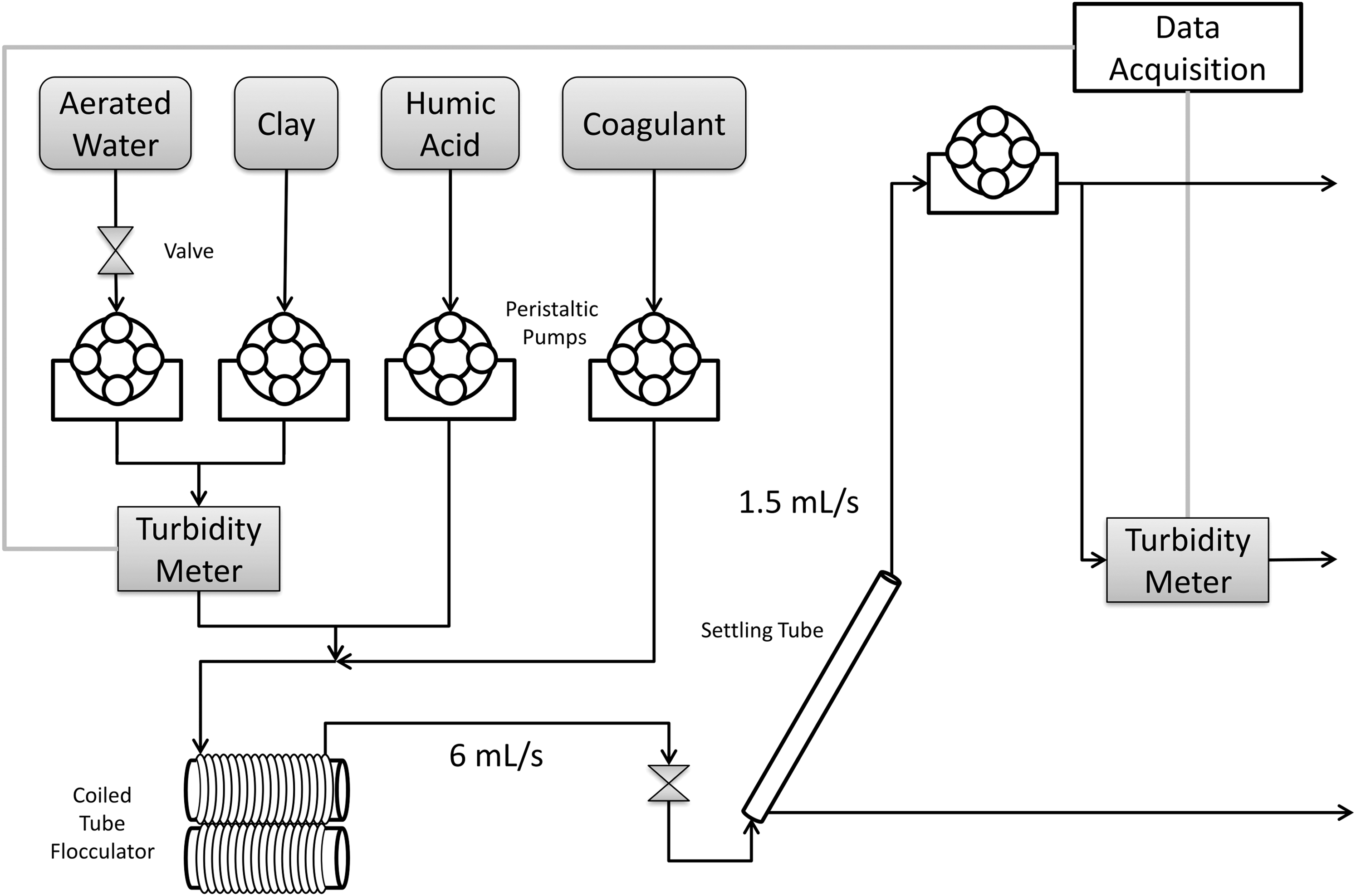
Experiments were conducted using the laboratory apparatus illustrated in Fig. 1. Cornell University tap water treated with granular activated carbon to remove preexisting DOM was pumped from an aerated and temperature-controlled reservoir and mixed with a concentrated stock suspension of kaolinite clay (R.T. Vanderbilt Co., Inc.) with average diameter of ∼7 μm (Sun et al., 2015; Wei et al., 2015) to form a feedback-regulated constant turbidity raw water source (Weber-Shirk, 2016). Reported Cornell University tap water characteristics are given in Table 1.

OPEN IN VIEWER

FIG. 1.

Experimental system schematic.

The humic substances used in experiments were obtained in the form of sodium salt from Sigma-Aldrich (H16752) and dissolved (solubility of 369 g/L at 20°C) in tap water to form the stock (Sigma-Aldrich, 2014). The stock was mixed with the raw water source to produce HA concentrations ranging from 0 to 15 mg/L (mass as salt). PACl coagulant doses (Holland Company, Adams, MA) ranging from 0.53 to 2.65 mg/L as Al were used to treat the synthetic raw water. The coagulant dosage and HA concentrations were regulated by adjusting the rotation speed of separate peristaltic pumps. The pH of the treated effluent was monitored in each experiment and was 7.5 ± 0.3. Influent turbidities of 50 nephelometric turbidity units (NTU) and 100 NTU were tested. Flocculation was accomplished by laminar flow through a coiled 9.52 mm inner diameter tube. The average velocity gradient in the coiled flocculator, \documentclass{aastex}\usepackage{amsbsy}\usepackage{amsfonts}\usepackage{amssymb}\usepackage{bm}\usepackage{mathrsfs}\usepackage{pifont}\usepackage{stmaryrd}\usepackage{textcomp}\usepackage{portland, xspace}\usepackage{amsmath, amsxtra}\usepackage{upgreek}\pagestyle{empty}\DeclareMathSizes{10}{9}{7}{6}\begin{document} $$\overline G$$ \end{document} , was calculated according the equation derived by Tse et al. (2011) as \documentclass{aastex}\usepackage{amsbsy}\usepackage{amsfonts}\usepackage{amssymb}\usepackage{bm}\usepackage{mathrsfs}\usepackage{pifont}\usepackage{stmaryrd}\usepackage{textcomp}\usepackage{portland, xspace}\usepackage{amsmath, amsxtra}\usepackage{upgreek}\pagestyle{empty}\DeclareMathSizes{10}{9}{7}{6}\begin{document} \begin{align*} { \overline G = { { \overline G } _ { { \rm { Straight } } } } \sqrt { 1 + 0.033 { { \left[ { { \rm log } \left( { { \frac { 4 { Q_ { { \rm { Plant } } } } } { \pi D \nu } } \sqrt { \frac { D } { { { R_ { \rm { c } } } } } } } \right) } \right] } ^4 } } , } \tag { 1 } \end{align*} \end{document}

where \documentclass{aastex}\usepackage{amsbsy}\usepackage{amsfonts}\usepackage{amssymb}\usepackage{bm}\usepackage{mathrsfs}\usepackage{pifont}\usepackage{stmaryrd}\usepackage{textcomp}\usepackage{portland, xspace}\usepackage{amsmath, amsxtra}\usepackage{upgreek}\pagestyle{empty}\DeclareMathSizes{10}{9}{7}{6}\begin{document} $${ \overline G_{{ \rm{Straight}}}}$$ \end{document} is fluid velocity gradient in a straight tube, Q_Plant is the experimental flow rate, D is the inner diameter of the flocculator tube, R_c is the diameter of curvature of the flocculator coils, and v is the kinematic viscosity of water, which is about \documentclass{aastex}\usepackage{amsbsy}\usepackage{amsfonts}\usepackage{amssymb}\usepackage{bm}\usepackage{mathrsfs}\usepackage{pifont}\usepackage{stmaryrd}\usepackage{textcomp}\usepackage{portland, xspace}\usepackage{amsmath, amsxtra}\usepackage{upgreek}\pagestyle{empty}\DeclareMathSizes{10}{9}{7}{6}\begin{document} $$1 \times \; { 10^ { - 6 } } { \frac { { { \rm { m } } ^2 } } { \rm { s } } } $$ \end{document} at 20°C (Kundu and Cohen, 2008). The overall experimental flow rate was 6 mL/s and the diameter of curvature of the coiled tubing (D_c) was 15 cm.

The value of \documentclass{aastex}\usepackage{amsbsy}\usepackage{amsfonts}\usepackage{amssymb}\usepackage{bm}\usepackage{mathrsfs}\usepackage{pifont}\usepackage{stmaryrd}\usepackage{textcomp}\usepackage{portland, xspace}\usepackage{amsmath, amsxtra}\usepackage{upgreek}\pagestyle{empty}\DeclareMathSizes{10}{9}{7}{6}\begin{document} $${ \overline G_{{ \rm{Straight}}}}$$ \end{document} was calculated by first estimating the head loss in a straight tube of the equivalent diameter, length, and material using the Hagen–Poiseuille equation for laminar flow: \documentclass{aastex}\usepackage{amsbsy}\usepackage{amsfonts}\usepackage{amssymb}\usepackage{bm}\usepackage{mathrsfs}\usepackage{pifont}\usepackage{stmaryrd}\usepackage{textcomp}\usepackage{portland, xspace}\usepackage{amsmath, amsxtra}\usepackage{upgreek}\pagestyle{empty}\DeclareMathSizes{10}{9}{7}{6}\begin{document} \begin{align*} {h_{ \rm{L}}} = {{32 \nu \bar uL} \over {{D^2}g}} , \tag{2} \end{align*} \end{document}

where L is the length of the tube (25.45 m in these experiments), \documentclass{aastex}\usepackage{amsbsy}\usepackage{amsfonts}\usepackage{amssymb}\usepackage{bm}\usepackage{mathrsfs}\usepackage{pifont}\usepackage{stmaryrd}\usepackage{textcomp}\usepackage{portland, xspace}\usepackage{amsmath, amsxtra}\usepackage{upgreek}\pagestyle{empty}\DeclareMathSizes{10}{9}{7}{6}\begin{document} $$\bar u$$ \end{document} is the mean velocity (84 mm/s) of the flow, and g is the acceleration due to gravity (Granger, 1995). From this head loss, an average rate of the loss of kinetic energy, \documentclass{aastex}\usepackage{amsbsy}\usepackage{amsfonts}\usepackage{amssymb}\usepackage{bm}\usepackage{mathrsfs}\usepackage{pifont}\usepackage{stmaryrd}\usepackage{textcomp}\usepackage{portland, xspace}\usepackage{amsmath, amsxtra}\usepackage{upgreek}\pagestyle{empty}\DeclareMathSizes{10}{9}{7}{6}\begin{document} $$\bar \varepsilon$$ \end{document} , can be estimated using \documentclass{aastex}\usepackage{amsbsy}\usepackage{amsfonts}\usepackage{amssymb}\usepackage{bm}\usepackage{mathrsfs}\usepackage{pifont}\usepackage{stmaryrd}\usepackage{textcomp}\usepackage{portland, xspace}\usepackage{amsmath, amsxtra}\usepackage{upgreek}\pagestyle{empty}\DeclareMathSizes{10}{9}{7}{6}\begin{document} \begin{align*} {\bar \varepsilon} = {{g{h_{ \rm{L}}}} \over \theta }, \tag{3} \end{align*} \end{document}

where θ is the mean hydraulic residence time (Pennock et al., 2018). The hydraulic residence time was 302 s as calculated by \documentclass{aastex}\usepackage{amsbsy}\usepackage{amsfonts}\usepackage{amssymb}\usepackage{bm}\usepackage{mathrsfs}\usepackage{pifont}\usepackage{stmaryrd}\usepackage{textcomp}\usepackage{portland, xspace}\usepackage{amsmath, amsxtra}\usepackage{upgreek}\pagestyle{empty}\DeclareMathSizes{10}{9}{7}{6}\begin{document} \begin{align*} {\theta} = {L \over { \bar u}}. \tag{4} \end{align*} \end{document}

The energy dissipation rate, which was calculated to be 2.24 mW/kg, can be converted to velocity gradient, \documentclass{aastex}\usepackage{amsbsy}\usepackage{amsfonts}\usepackage{amssymb}\usepackage{bm}\usepackage{mathrsfs}\usepackage{pifont}\usepackage{stmaryrd}\usepackage{textcomp}\usepackage{portland, xspace}\usepackage{amsmath, amsxtra}\usepackage{upgreek}\pagestyle{empty}\DeclareMathSizes{10}{9}{7}{6}\begin{document} $$\overline G$$ \end{document} , by \documentclass{aastex}\usepackage{amsbsy}\usepackage{amsfonts}\usepackage{amssymb}\usepackage{bm}\usepackage{mathrsfs}\usepackage{pifont}\usepackage{stmaryrd}\usepackage{textcomp}\usepackage{portland, xspace}\usepackage{amsmath, amsxtra}\usepackage{upgreek}\pagestyle{empty}\DeclareMathSizes{10}{9}{7}{6}\begin{document} \begin{align*} {\overline G }= \sqrt {{{ \bar \varepsilon } \over \nu }} , \tag{5} \end{align*} \end{document}

which gave a velocity gradient of 50.1 s⁻¹. Using this value for \documentclass{aastex}\usepackage{amsbsy}\usepackage{amsfonts}\usepackage{amssymb}\usepackage{bm}\usepackage{mathrsfs}\usepackage{pifont}\usepackage{stmaryrd}\usepackage{textcomp}\usepackage{portland, xspace}\usepackage{amsmath, amsxtra}\usepackage{upgreek}\pagestyle{empty}\DeclareMathSizes{10}{9}{7}{6}\begin{document} $${ \overline G_{{ \rm{Straight}}}}$$ \end{document} in Equation (1) resulted in a value of 71.1 s⁻¹ for \documentclass{aastex}\usepackage{amsbsy}\usepackage{amsfonts}\usepackage{amssymb}\usepackage{bm}\usepackage{mathrsfs}\usepackage{pifont}\usepackage{stmaryrd}\usepackage{textcomp}\usepackage{portland, xspace}\usepackage{amsmath, amsxtra}\usepackage{upgreek}\pagestyle{empty}\DeclareMathSizes{10}{9}{7}{6}\begin{document} $$\overline G$$ \end{document} .

A coiled tube flocculator was used in this research because it is a high Péclet number reactor much like a baffled hydraulic flocculator and because the average velocity gradient in laminar tube flow is well defined (Weber-Shirk and Lion, 2010). After flowing through the flocculator, a fraction of the flow was passed through a tube settler and the settled water turbidity was recorded continuously for each experiment. The 1.37 m (4.5 ft) tube settler, with an inner diameter of 2.66 cm, had an entry port diameter of 0.95 cm (3/8 in) near the bottom and an exit port diameter of 0.635 cm (1/4 in) near the top. The capture velocity was controlled at 0.10 mm/s using a peristaltic pump with flow set by \documentclass{aastex}\usepackage{amsbsy}\usepackage{amsfonts}\usepackage{amssymb}\usepackage{bm}\usepackage{mathrsfs}\usepackage{pifont}\usepackage{stmaryrd}\usepackage{textcomp}\usepackage{portland, xspace}\usepackage{amsmath, amsxtra}\usepackage{upgreek}\pagestyle{empty}\DeclareMathSizes{10}{9}{7}{6}\begin{document} \begin{align*} {Q_ {\rm {S}}} = {{\pi} \over {4}} \;D_ { \rm { S } } ^2 { V_ { \rm { c } } } \left( { { \frac { { L_ { \rm { S } } } } { { D_ { \rm { S } } } } } \cos { \alpha _ { \rm { S } } } + \sin { \alpha_{ \rm { S } } } } \right) , \tag { 6 } \end{align*} \end{document}

where V_c is the capture velocity, L_S is the length of the tube settler, D_S is the diameter of the tube settler, and α_S is the angle of inclination of the tube settler, which was set at 60° (Schulz and Okun, 1984).

Model Formation

A flocculation model accounting for the effects of HA should predict the effective collisions between colloids for a given set of conditions. The dimensionless product of the fluid velocity gradient and mean hydraulic residence time, \documentclass{aastex}\usepackage{amsbsy}\usepackage{amsfonts}\usepackage{amssymb}\usepackage{bm}\usepackage{mathrsfs}\usepackage{pifont}\usepackage{stmaryrd}\usepackage{textcomp}\usepackage{portland, xspace}\usepackage{amsmath, amsxtra}\usepackage{upgreek}\pagestyle{empty}\DeclareMathSizes{10}{9}{7}{6}\begin{document} $$\overline G \theta$$ \end{document} , has been used as a measure of the collision potential provided by a flocculator that experiences laminar flow (Camp, 1953; Cleasby, 1984). It is well known that not all collisions between suspended particles result in aggregation, and average attachment efficiency, \documentclass{aastex}\usepackage{amsbsy}\usepackage{amsfonts}\usepackage{amssymb}\usepackage{bm}\usepackage{mathrsfs}\usepackage{pifont}\usepackage{stmaryrd}\usepackage{textcomp}\usepackage{portland, xspace}\usepackage{amsmath, amsxtra}\usepackage{upgreek}\pagestyle{empty}\DeclareMathSizes{10}{9}{7}{6}\begin{document} $$\bar \alpha$$ \end{document} , has been used to denote the fraction of successful collisions (Letterman, 1999).

The initial primary particle volume fraction, φ₀, also influences coagulation (Ives, 1968; O'Melia, 1972) and gives the fraction of the volume of the suspension occupied by the influent primary particles, \documentclass{aastex}\usepackage{amsbsy}\usepackage{amsfonts}\usepackage{amssymb}\usepackage{bm}\usepackage{mathrsfs}\usepackage{pifont}\usepackage{stmaryrd}\usepackage{textcomp}\usepackage{portland, xspace}\usepackage{amsmath, amsxtra}\usepackage{upgreek}\pagestyle{empty}\DeclareMathSizes{10}{9}{7}{6}\begin{document} \begin{align*} {\phi_0} = { \frac {{ C_0}} {{ \rho _ { \rm {P}}}}} , \tag { 7 } \end{align*} \end{document}

where C₀ is the influent particle concentration (kaolinite clay in these experiments) and ρ_P is the density of influent particles (Swetland et al., 2014).

In laminar-flow flocculators, the velocity of one particle relative to another scales with the average separation distance between particles (Swetland et al., 2014). The time between interparticle collisions is inversely proportional to both φ and the relative velocity between particles. As the relative velocity between particles is proportional to separation distance, the time between collisions is proportional to \documentclass{aastex}\usepackage{amsbsy}\usepackage{amsfonts}\usepackage{amssymb}\usepackage{bm}\usepackage{mathrsfs}\usepackage{pifont}\usepackage{stmaryrd}\usepackage{textcomp}\usepackage{portland, xspace}\usepackage{amsmath, amsxtra}\usepackage{upgreek}\pagestyle{empty}\DeclareMathSizes{10}{9}{7}{6}\begin{document} $$ { \phi ^ { \frac { 1 } { 3 } } } $$ \end{document} , and the average separation distance, \documentclass{aastex}\usepackage{amsbsy}\usepackage{amsfonts}\usepackage{amssymb}\usepackage{bm}\usepackage{mathrsfs}\usepackage{pifont}\usepackage{stmaryrd}\usepackage{textcomp}\usepackage{portland, xspace}\usepackage{amsmath, amsxtra}\usepackage{upgreek}\pagestyle{empty}\DeclareMathSizes{10}{9}{7}{6}\begin{document} $${ \rm{ \overline \Lambda }}$$ \end{document} , is given by \documentclass{aastex}\usepackage{amsbsy}\usepackage{amsfonts}\usepackage{amssymb}\usepackage{bm}\usepackage{mathrsfs}\usepackage{pifont}\usepackage{stmaryrd}\usepackage{textcomp}\usepackage{portland, xspace}\usepackage{amsmath, amsxtra}\usepackage{upgreek}\pagestyle{empty}\DeclareMathSizes{10}{9}{7}{6}\begin{document} \begin{align*} {{\overline \Lambda}} = {d_{\rm {P}}} \left({\frac {\pi} {{6 \phi }}} \right) ^ {\frac {1}{3}}. \tag {8} \end{align*} \end{document}

The result is that, for laminar flow, the average time for primary particle collisions scales with \documentclass{aastex}\usepackage{amsbsy}\usepackage{amsfonts}\usepackage{amssymb}\usepackage{bm}\usepackage{mathrsfs}\usepackage{pifont}\usepackage{stmaryrd}\usepackage{textcomp}\usepackage{portland, xspace}\usepackage{amsmath, amsxtra}\usepackage{upgreek}\pagestyle{empty}\DeclareMathSizes{10}{9}{7}{6}\begin{document} $$\phi _0^ { - \frac { 2 } { 3 } } $$ \end{document} (Weber-Shirk and Lion, 2010). Because performance is proportional to the average number of collisions a primary particle undergoes, and as the number of collisions is inversely proportional to the average time between collisions, the final performance is proportional to \documentclass{aastex}\usepackage{amsbsy}\usepackage{amsfonts}\usepackage{amssymb}\usepackage{bm}\usepackage{mathrsfs}\usepackage{pifont}\usepackage{stmaryrd}\usepackage{textcomp}\usepackage{portland, xspace}\usepackage{amsmath, amsxtra}\usepackage{upgreek}\pagestyle{empty}\DeclareMathSizes{10}{9}{7}{6}\begin{document} $$\phi _0^ { \frac { 2 } { 3 } } $$ \end{document} (Pennock et al., 2018).

A laminar-flow hydraulic flocculator model was developed and validated based on the above analysis in Pennock et al. (2018) with the form \documentclass{aastex}\usepackage{amsbsy}\usepackage{amsfonts}\usepackage{amssymb}\usepackage{bm}\usepackage{mathrsfs}\usepackage{pifont}\usepackage{stmaryrd}\usepackage{textcomp}\usepackage{portland, xspace}\usepackage{amsmath, amsxtra}\usepackage{upgreek}\pagestyle{empty}\DeclareMathSizes{10}{9}{7}{6}\begin{document} \begin{align*} {p{C^{*}}} = \frac { 3 } { 2 } { { \log } _ { 10 } } \left[ {\frac { 2 } { 3 } { { \left( { \frac { 6 } { \pi } } \right) } ^{ \frac { 2 } { 3 } } } \pi k \overline { \alpha } \overline { G } \theta \phi _0^ { \frac { 2 } { 3 } } + 1 } \right] , \tag {9} \end{align*} \end{document}

where k is a fitting parameter dependent on the value of V_c used for sedimentation, \documentclass{aastex}\usepackage{amsbsy}\usepackage{amsfonts}\usepackage{amssymb}\usepackage{bm}\usepackage{mathrsfs}\usepackage{pifont}\usepackage{stmaryrd}\usepackage{textcomp}\usepackage{portland, xspace}\usepackage{amsmath, amsxtra}\usepackage{upgreek}\pagestyle{empty}\DeclareMathSizes{10}{9}{7}{6}\begin{document} $$\bar \alpha$$ \end{document} is the mean fraction of collisions that are successful (i.e., result in aggregation), and pC* is defined as \documentclass{aastex}\usepackage{amsbsy}\usepackage{amsfonts}\usepackage{amssymb}\usepackage{bm}\usepackage{mathrsfs}\usepackage{pifont}\usepackage{stmaryrd}\usepackage{textcomp}\usepackage{portland, xspace}\usepackage{amsmath, amsxtra}\usepackage{upgreek}\pagestyle{empty}\DeclareMathSizes{10}{9}{7}{6}\begin{document} \begin{align*} {p{ C^*}} = - \log \left( { { \frac { { \rm { Effluent \;Turbidity } } } { { \rm { Influent \;Turbidity } } } }} \right) . \tag {10} \end{align*} \end{document}

Equation (9), referred to as the AguaClara flocculation model in Pennock et al. (2018), is a Lagrangian hydrodynamic model that assumes that the aggregation of primary particles is rate limiting. It further assumes that these particles, on average, will collide when the volume of fluid swept out as one particle approaches the other is equal to the average volume occupied by a single particle in the suspension. The time for these collisions to occur increases as flocculation proceeds, since the concentration of primary particles decreases in a way that is assumed to be first order with respect to collisions. Thus, with each successive collision, the average volume occupied by primary particles increases, and it takes longer for the next collision to occur. In Equation (9), performance is linearly proportional to the logarithm of the effective collision potential, \documentclass{aastex}\usepackage{amsbsy}\usepackage{amsfonts}\usepackage{amssymb}\usepackage{bm}\usepackage{mathrsfs}\usepackage{pifont}\usepackage{stmaryrd}\usepackage{textcomp}\usepackage{portland, xspace}\usepackage{amsmath, amsxtra}\usepackage{upgreek}\pagestyle{empty}\DeclareMathSizes{10}{9}{7}{6}\begin{document} $$\log \left( { \overline {\alpha}} {\overline {G}} \theta \phi _0^{2/3} \right)$$ \end{document} .

This group of parameters is the same as the group first described by Swetland et al. (2014), with the exception that they used the estimated fractional coverage of the colloid surface by coagulant, \documentclass{aastex}\usepackage{amsbsy}\usepackage{amsfonts}\usepackage{amssymb}\usepackage{bm}\usepackage{mathrsfs}\usepackage{pifont}\usepackage{stmaryrd}\usepackage{textcomp}\usepackage{portland, xspace}\usepackage{amsmath, amsxtra}\usepackage{upgreek}\pagestyle{empty}\DeclareMathSizes{10}{9}{7}{6}\begin{document} $${{ \rm{ \overline \Gamma }}_{{ \rm{PACl}} - { \rm{Clay}}}}$$ \end{document} , as a measure of attachment efficiency instead of \documentclass{aastex}\usepackage{amsbsy}\usepackage{amsfonts}\usepackage{amssymb}\usepackage{bm}\usepackage{mathrsfs}\usepackage{pifont}\usepackage{stmaryrd}\usepackage{textcomp}\usepackage{portland, xspace}\usepackage{amsmath, amsxtra}\usepackage{upgreek}\pagestyle{empty}\DeclareMathSizes{10}{9}{7}{6}\begin{document} $$\bar \alpha$$ \end{document} . Pennock et al. (2018) recognized that surface coverage of both particles participating in a collision matters and introduced \documentclass{aastex}\usepackage{amsbsy}\usepackage{amsfonts}\usepackage{amssymb}\usepackage{bm}\usepackage{mathrsfs}\usepackage{pifont}\usepackage{stmaryrd}\usepackage{textcomp}\usepackage{portland, xspace}\usepackage{amsmath, amsxtra}\usepackage{upgreek}\pagestyle{empty}\DeclareMathSizes{10}{9}{7}{6}\begin{document} $$\bar \alpha$$ \end{document} to convert the geometric information contained in \documentclass{aastex}\usepackage{amsbsy}\usepackage{amsfonts}\usepackage{amssymb}\usepackage{bm}\usepackage{mathrsfs}\usepackage{pifont}\usepackage{stmaryrd}\usepackage{textcomp}\usepackage{portland, xspace}\usepackage{amsmath, amsxtra}\usepackage{upgreek}\pagestyle{empty}\DeclareMathSizes{10}{9}{7}{6}\begin{document} $${{ \rm{ \overline \Gamma }}_{{ \rm{PACl}} - { \rm{Clay}}}}$$ \end{document} to a probability of a successful collision. Using data gathered by Swetland et al. (2014), Pennock et al. (2018) were able to predict the results of independent laminar flocculation experiments with no adjustable parameters in the absence of added DOM.

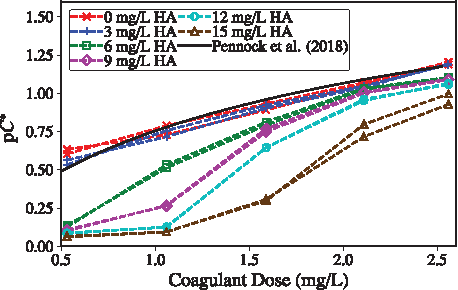
Experimental results obtained with added HA present are given in Fig. 3 along with predictions based on the AguaClara flocculation model [Eq. (9)]. It was evident that the attachment efficiency was adversely affected by the addition of HA. Referencing adsorption measurements by Davis (1982), a minority (his study found 20%) of added DOM would be adsorbed by kaolinite at the experimental pH of 7.5. Thus, most HA macromolecules were available to attach to the added coagulant nanoparticles, and for the purpose of this model, it was assumed that the HA did not adsorb to the kaolinite. The following simplifying assumptions were made to account for the presence of HAs: (1) HA macromolecules attach only to coagulant nanoparticles to form nanoaggregates, (2) nanoaggregates attach both to clay and to the reactor walls in proportion to the relative amount of surface area of each, and (3) the surfaces of precipitated coagulant nanoparticles promote adhesion while the surfaces of bound HAs prevent adhesion.

In this study, HA macromolecules and PACl nanoparticles were modeled as spheres. Based on the size of coagulant nanoparticles and HA macromolecules, their number concentrations, N_HA and N_PACl, respectively, can be estimated by \documentclass{aastex}\usepackage{amsbsy}\usepackage{amsfonts}\usepackage{amssymb}\usepackage{bm}\usepackage{mathrsfs}\usepackage{pifont}\usepackage{stmaryrd}\usepackage{textcomp}\usepackage{portland, xspace}\usepackage{amsmath, amsxtra}\usepackage{upgreek}\pagestyle{empty}\DeclareMathSizes{10}{9}{7}{6}\begin{document} \begin{align*} {N_{{\rm {HA}}}} = { \frac { { C_ { { \rm { HA } } } } } { { \rho_ { { \rm { HA } } } } \frac { \pi } { 6 } d_ { { \rm { HA } } }^3 } } , \tag {11} \end{align*} \end{document}

and \documentclass{aastex}\usepackage{amsbsy}\usepackage{amsfonts}\usepackage{amssymb}\usepackage{bm}\usepackage{mathrsfs}\usepackage{pifont}\usepackage{stmaryrd}\usepackage{textcomp}\usepackage{portland, xspace}\usepackage{amsmath, amsxtra}\usepackage{upgreek}\pagestyle{empty}\DeclareMathSizes{10}{9}{7}{6}\begin{document} \begin{align*} {N_{{ \rm{PACI}}}} = {{{C_{{ \rm{PACl}}}}} \over {{ \rho _{{\rm{PACl}}}}{ \pi \over 6}d_{{ \rm{PACl}}}^3}} , \tag{12} \end{align*} \end{document}

where C_PACl is the dose of coagulant in mg/L as Al; C_HA is the concentration of HA salt in mg/L; ρ_PACl is the density of the coagulant [Swetland et al. (2013) found 1,138 kg/m³]; ρ_HA is the density of HA salt, 1,520 kg/m³ (Sigma-Aldrich, 2014); d_HA is the diameter of HA macromolecules (an adjustable model parameter); and d_PACl is the diameter of precipitated PACl coagulant nanoparticles, taken to be 90 nm as found by Garland (2017).

A key model assumption was that HA macromolecules cannot adhere to a coagulant surface that is occupied by an HA macromolecule, as HA macromolecules are assumed to not appreciably self aggregate. Li et al. (2018) observed that for HA adsorption onto Al₂O₃ surfaces, the macromolecules adsorbed in a monolayer. The outcome of this assumption is that HA macromolecules attach to an uncovered surface of coagulant and do not stack on top of one another. The available surface area of the PACl nanoparticle was modeled as the surface area of an equivalent sphere. The amount of that area that is occupied by an attached HA macromolecule was estimated as the projected area of a sphere with volume equivalent to an HA macromolecule. A new variable describing the coverage of coagulant nanoparticle surface area by HA macromolecules, \documentclass{aastex}\usepackage{amsbsy}\usepackage{amsfonts}\usepackage{amssymb}\usepackage{bm}\usepackage{mathrsfs}\usepackage{pifont}\usepackage{stmaryrd}\usepackage{textcomp}\usepackage{portland, xspace}\usepackage{amsmath, amsxtra}\usepackage{upgreek}\pagestyle{empty}\DeclareMathSizes{10}{9}{7}{6}\begin{document} \begin{align*} { \rm { \overline \Gamma } } { { \rm { } } _ { { \rm { HA } } - { \rm { PACl } } } } = { \frac { \frac { \pi } { 4 } d_ { { \rm { HA } } } ^2 } { \pi d_ { { \rm { PACl } } } ^2 } } { \frac { { N_ { { \rm { HA } } } } } { { N_ { { \rm { PACl } } } } } } , \tag { 13 } \end{align*} \end{document}

was created to be incorporated into the model (within \documentclass{aastex}\usepackage{amsbsy}\usepackage{amsfonts}\usepackage{amssymb}\usepackage{bm}\usepackage{mathrsfs}\usepackage{pifont}\usepackage{stmaryrd}\usepackage{textcomp}\usepackage{portland, xspace}\usepackage{amsmath, amsxtra}\usepackage{upgreek}\pagestyle{empty}\DeclareMathSizes{10}{9}{7}{6}\begin{document} $$\bar \alpha$$ \end{document} ). The maximum value of \documentclass{aastex}\usepackage{amsbsy}\usepackage{amsfonts}\usepackage{amssymb}\usepackage{bm}\usepackage{mathrsfs}\usepackage{pifont}\usepackage{stmaryrd}\usepackage{textcomp}\usepackage{portland, xspace}\usepackage{amsmath, amsxtra}\usepackage{upgreek}\pagestyle{empty}\DeclareMathSizes{10}{9}{7}{6}\begin{document} $${ \rm{ \overline \Gamma }}{{ \rm{ }}_{{ \rm{HA}} - { \rm{PACl}}}}$$ \end{document} is 1, which reflects the assumption that HA does not continue to affect coagulation performance beyond completely coating the coagulant precipitates.

The first two steps in particle aggregation, where HA macromolecules attach to coagulant nanoparticles and then the resulting nanoaggregates attach to clay surfaces, were assumed to be rapid because diffusion is an effective transport process for nanoparticles (Benjamin and Lawler, 2013). Subsequent to rapid mix, the clay particles with attached nanoaggregates undergo collisions during the flocculation process and the aggregation process is governed by fluid shear (Pennock et al., 2018). The success of a collision between clay particles is hypothesized to be dependent on the properties of the contact surfaces at the initial point of contact.

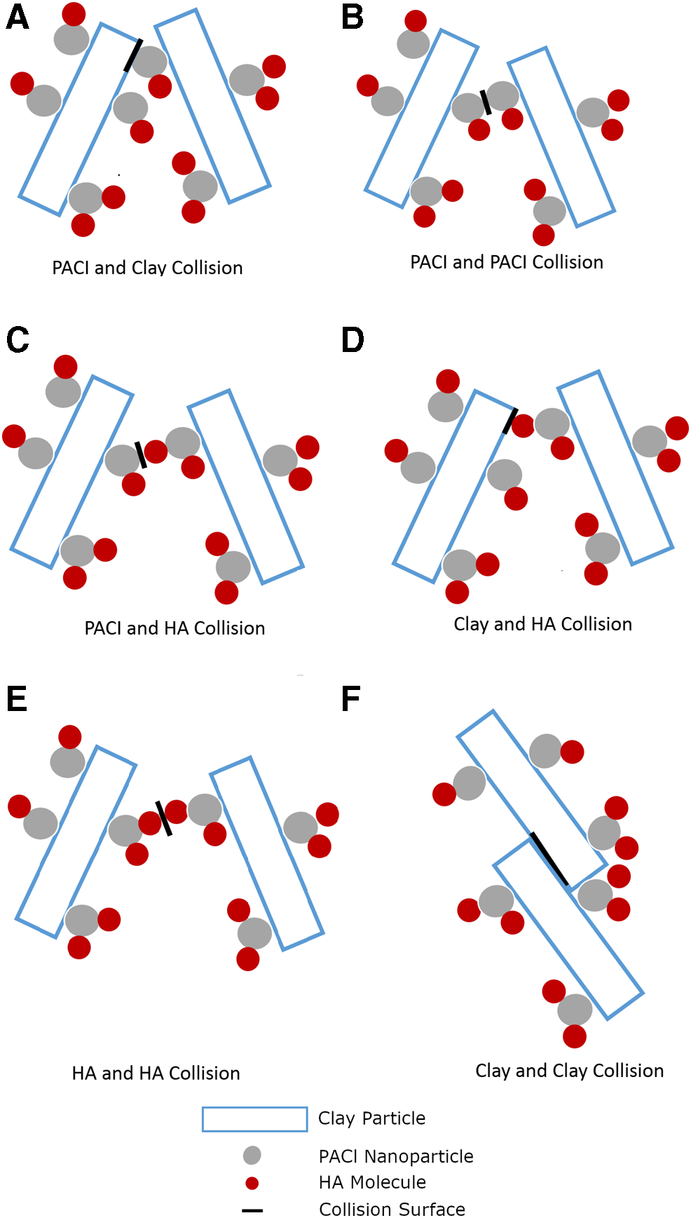
The three types of surfaces (PACl, HA, and clay) have 6 (3!) potential interactions as given in Fig. 2.

OPEN IN VIEWER

FIG. 2.

Modes of collision between particles during flocculation. Modes (A) through (C) are considered successful collisions because they include at least one coagulant precipitate at the point of contact. Modes (D) through (F) are considered unsuccessful collisions because they do not.

Of these interactions considered in the model, the collisions that will result in attachment were assumed to involve at least one PACl nanoparticle surface (Fig. 2A–C). The attachment efficiency was hypothesized to be the sum of probability of these three types of collisions, formally expressed as: \documentclass{aastex}\usepackage{amsbsy}\usepackage{amsfonts}\usepackage{amssymb}\usepackage{bm}\usepackage{mathrsfs}\usepackage{pifont}\usepackage{stmaryrd}\usepackage{textcomp}\usepackage{portland, xspace}\usepackage{amsmath, amsxtra}\usepackage{upgreek}\pagestyle{empty}\DeclareMathSizes{10}{9}{7}{6}\begin{document} \begin{align*} {\bar \alpha} = {{ \bar \alpha }_{{ \rm{PACl}} - { \rm{Clay}}}} + {{ \bar \alpha }_{{ \rm{PACl}} - { \rm{PACl}}}} + {{ \bar \alpha }_{{ \rm{HA}} - { \rm{PACl}}}} , \tag{14} \end{align*} \end{document}

where the subscripts define the two surfaces that are interacting. The overbars indicate that all these represent mean probabilities for an entire suspension rather than the probabilities for specific particles.

The probability of a clay surface colliding with a PACl surface (Fig. 2A) is equal to twice the probability that the first surface is clay \documentclass{aastex}\usepackage{amsbsy}\usepackage{amsfonts}\usepackage{amssymb}\usepackage{bm}\usepackage{mathrsfs}\usepackage{pifont}\usepackage{stmaryrd}\usepackage{textcomp}\usepackage{portland, xspace}\usepackage{amsmath, amsxtra}\usepackage{upgreek}\pagestyle{empty}\DeclareMathSizes{10}{9}{7}{6}\begin{document} $$\left( {1 - {{{ \rm{ \overline \Gamma }}}_{{ \rm{PACl}} - {\rm{Clay}}}}} \right)$$ \end{document} and the second surface is the PACl surface of a PACl-HA nanoaggregate \documentclass{aastex}\usepackage{amsbsy}\usepackage{amsfonts}\usepackage{amssymb}\usepackage{bm}\usepackage{mathrsfs}\usepackage{pifont}\usepackage{stmaryrd}\usepackage{textcomp}\usepackage{portland, xspace}\usepackage{amsmath, amsxtra}\usepackage{upgreek}\pagestyle{empty}\DeclareMathSizes{10}{9}{7}{6}\begin{document} $$\left[ { \left( {1 - {{{ \rm{ \overline \Gamma }}}_{{ \rm{HA}} - { \rm{PACl}}}}} \right) {{{ \rm{ \overline \Gamma }}}_{{ \rm{PACl}} - { \rm{Clay}}}}} \right]$$ \end{document} , as either of two colliding particles could provide the clay surface or the PACl surface, \documentclass{aastex}\usepackage{amsbsy}\usepackage{amsfonts}\usepackage{amssymb}\usepackage{bm}\usepackage{mathrsfs}\usepackage{pifont}\usepackage{stmaryrd}\usepackage{textcomp}\usepackage{portland, xspace}\usepackage{amsmath, amsxtra}\usepackage{upgreek}\pagestyle{empty}\DeclareMathSizes{10}{9}{7}{6}\begin{document} \begin{align*} {{ \bar \alpha}_{{ \rm{PACl}} - { \rm{Clay}}}} = 2 \left( {1 - {{{{\overline \Gamma }}}_{{ \rm{PACl}} - { \rm{Clay}}}}} \right) \left[ { \left( {1 - {{{{ \overline {\Gamma} }}}_{{ \rm{HA}} - { \rm{PACl}}}}} \right) {{{{ \overline \Gamma }}}_{{ \rm{PACl}} - { \rm{Clay}}}}} \right] . \tag{15} \end{align*} \end{document}

The probability of a collision between the PACl surfaces of two PACl-HA nanoaggregates \documentclass{aastex}\usepackage{amsbsy}\usepackage{amsfonts}\usepackage{amssymb}\usepackage{bm}\usepackage{mathrsfs}\usepackage{pifont}\usepackage{stmaryrd}\usepackage{textcomp}\usepackage{portland, xspace}\usepackage{amsmath, amsxtra}\usepackage{upgreek}\pagestyle{empty}\DeclareMathSizes{10}{9}{7}{6}\begin{document} $$\left[ { \left( {1 - {{{ \rm{ \overline \Gamma }}}_{{ \rm{HA}} - { \rm{PACl}}}}} \right) {{{ \rm{ \overline \Gamma }}}_{{ \rm{PACl}} - { \rm{Clay}}}}} \right]$$ \end{document} (Fig. 2B) is given by \documentclass{aastex}\usepackage{amsbsy}\usepackage{amsfonts}\usepackage{amssymb}\usepackage{bm}\usepackage{mathrsfs}\usepackage{pifont}\usepackage{stmaryrd}\usepackage{textcomp}\usepackage{portland, xspace}\usepackage{amsmath, amsxtra}\usepackage{upgreek}\pagestyle{empty}\DeclareMathSizes{10}{9}{7}{6}\begin{document} \begin{align*} {{ \bar \alpha }_{{ \rm{PACl}} - { \rm{PACI}}}} = {{ \left[ { \left( {1 - {{{{\overline \Gamma }}}_{{ \rm{HA}} - {\rm{PACl}}}}} \right) {{{{\overline \Gamma }}}_{{ \rm{PACl}} - {\rm{Clay}}}}} \right] }^2}. \tag{16} \end{align*} \end{document}

The probability of a collision between a PACl surface of a PACl-HA nanoaggregate \documentclass{aastex}\usepackage{amsbsy}\usepackage{amsfonts}\usepackage{amssymb}\usepackage{bm}\usepackage{mathrsfs}\usepackage{pifont}\usepackage{stmaryrd}\usepackage{textcomp}\usepackage{portland, xspace}\usepackage{amsmath, amsxtra}\usepackage{upgreek}\pagestyle{empty}\DeclareMathSizes{10}{9}{7}{6}\begin{document} $$\left[ { \left( {1 - {{{ \rm{ \overline \Gamma }}}_{{ \rm{HA}} - { \rm{PACl}}}}} \right) {{{ \rm{ \overline \Gamma }}}_{{\rm{PACl}} - { \rm{Clay}}}}} \right]$$ \end{document} and an HA surface of a PACl-HA nanoaggregate \documentclass{aastex}\usepackage{amsbsy}\usepackage{amsfonts}\usepackage{amssymb}\usepackage{bm}\usepackage{mathrsfs}\usepackage{pifont}\usepackage{stmaryrd}\usepackage{textcomp}\usepackage{portland, xspace}\usepackage{amsmath, amsxtra}\usepackage{upgreek}\pagestyle{empty}\DeclareMathSizes{10}{9}{7}{6}\begin{document} $$\left( {{{{ \rm{ \overline \Gamma }}}_{{ \rm{HA}} - {\rm{PACl}}}}{{{ \rm{ \overline \Gamma }}}_{{ \rm{PACl}} - {\rm{Clay}}}}} \right)$$ \end{document} (Fig. 2C), or vice versa, is given by \documentclass{aastex}\usepackage{amsbsy}\usepackage{amsfonts}\usepackage{amssymb}\usepackage{bm}\usepackage{mathrsfs}\usepackage{pifont}\usepackage{stmaryrd}\usepackage{textcomp}\usepackage{portland, xspace}\usepackage{amsmath, amsxtra}\usepackage{upgreek}\pagestyle{empty}\DeclareMathSizes{10}{9}{7}{6}\begin{document} \begin{align*} \begin{split} & {{ \bar \alpha }_{{\rm{HA}} - { \rm{PACl}}}} = 2 \left[ {\overline {\Gamma}}_{{ \rm{PACl}} - {\rm{Clay}}} \left( {1 - {{\overline \Gamma}}_{{ \rm{HA}} - \rm{PACl}}} \right) \right] \\ & \left[ {\overline {\Gamma}}_{{\rm{HA}} - { \rm{PACl}}} { \overline {\Gamma}}_{{\rm{PACl}} - {\rm{Clay}}} \right] , \\ \end{split} \tag{17} \end{align*} \end{document}

where the factor of two accounts for the possibility that either colliding particle could contribute either surface type. The model accounting for the presence of HAs was modified from the Pennock et al. (2018) model by redefining the attachment efficiency, \documentclass{aastex}\usepackage{amsbsy}\usepackage{amsfonts}\usepackage{amssymb}\usepackage{bm}\usepackage{mathrsfs}\usepackage{pifont}\usepackage{stmaryrd}\usepackage{textcomp}\usepackage{portland, xspace}\usepackage{amsmath, amsxtra}\usepackage{upgreek}\pagestyle{empty}\DeclareMathSizes{10}{9}{7}{6}\begin{document} $$\bar \alpha$$ \end{document} , using Equation (14) to account for the presence of HA.

The physical properties of HA vary with composition. The diameter of HA macromolecules is estimated to range from 4 to 110 nm (Österberg et al., 1993). Because of the variation in the size of HA macromolecules, the characteristic diameter of the HA macromolecules was used as a fitting parameter. Thus, there are two adjustable model parameters, k [Eq. (9)], which accounts for the sedimentation capture velocity, and d_HA, which accounts for coagulant precipitate surface coverage by HA. These parameters were fit to results from observations taken with an influent turbidity of 50 NTU; the model was then validated by independently predicting results from experiments with an influent turbidity of 100 NTU.

Results

The results from 60 experiments, transformed by Equation (10), are given in Fig. 3 for an inflow turbidity of 50 NTU with PACl doses ranging from 0.53 to 2.65 mg/L as Al and HA concentration ranging from 0 to 15 mg/L. A capture velocity of 0.10 mm/s was used in the experiments, which is a conservatively designed lamellar settler capture velocity (Willis, 1978). Experiments were replicated for each combination of HA and PACl dose.

OPEN IN VIEWER

FIG. 3.

\documentclass{aastex}\usepackage{amsbsy}\usepackage{amsfonts}\usepackage{amssymb}\usepackage{bm}\usepackage{mathrsfs}\usepackage{pifont}\usepackage{stmaryrd}\usepackage{textcomp}\usepackage{portland, xspace}\usepackage{amsmath, amsxtra}\usepackage{upgreek}\pagestyle{empty}\DeclareMathSizes{10}{9}{7}{6}\begin{document} $${ \rm{p}}{C^*}$$ \end{document} as a function of coagulant dose for 50 NTU influent turbidity. HA, humic acid; NTU, nephelometric turbidity units.

The data show that increased coagulant dose is positively correlated with turbidity removal. The effluent turbidity was greatly increased by the presence of HA. Also shown is a model fit using the AguaClara flocculation model given by Pennock et al. (2018). As shown, the model can fit the performance of the 0 mg/L HA data and even the 3 mg/L HA data reasonably well, but increasing doses of HA decrease performance appreciably, necessitating a modification to the original model.

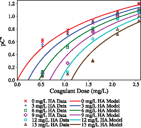
To apply the modified model to the raw data, the data points with 0 mg/L HA were fit by k, as their performance was not influenced by d_HA, resulting in k = 0.16. Then, the remaining data were fit using d_HA (with the previously determined k value) to minimize the sum squared error, resulting in d_HA = 75 nm with a pC* (dimensionless) root mean square error (RMSE), of 0.08. To avoid biasing the fit by data for which the coagulant dose was insufficient to overcome the effect of HA, data with performance lower than pC* = 0.25 were neglected for the fitting. Figure 4 shows the fit of the model to the observations for the 50 NTU experiments. The offset of the model lines from an intercept on the abscissa at 0 mg/L as Al coagulant dose is a result of \documentclass{aastex}\usepackage{amsbsy}\usepackage{amsfonts}\usepackage{amssymb}\usepackage{bm}\usepackage{mathrsfs}\usepackage{pifont}\usepackage{stmaryrd}\usepackage{textcomp}\usepackage{portland, xspace}\usepackage{amsmath, amsxtra}\usepackage{upgreek}\pagestyle{empty}\DeclareMathSizes{10}{9}{7}{6}\begin{document} $${{\overline \Gamma }}_{{ \rm{HA}} - { \rm{PACl}}}$$ \end{document} being 1 (i.e., complete coverage of PACl precipitates by HA macromolecules) for coagulant doses below the intercept value.

OPEN IN VIEWER

FIG. 4.

Model fit for \documentclass{aastex}\usepackage{amsbsy}\usepackage{amsfonts}\usepackage{amssymb}\usepackage{bm}\usepackage{mathrsfs}\usepackage{pifont}\usepackage{stmaryrd}\usepackage{textcomp}\usepackage{portland, xspace}\usepackage{amsmath, amsxtra}\usepackage{upgreek}\pagestyle{empty}\DeclareMathSizes{10}{9}{7}{6}\begin{document} $${ \rm{p}}{C^*}$$ \end{document} as function of coagulant dose for 50 NTU raw water turbidity.

With the given fitted value of d_HA = 75 nm for the 50 NTU influent turbidity data set, the coverage of coagulant nanoparticle surfaces by HA \documentclass{aastex}\usepackage{amsbsy}\usepackage{amsfonts}\usepackage{amssymb}\usepackage{bm}\usepackage{mathrsfs}\usepackage{pifont}\usepackage{stmaryrd}\usepackage{textcomp}\usepackage{portland, xspace}\usepackage{amsmath, amsxtra}\usepackage{upgreek}\pagestyle{empty}\DeclareMathSizes{10}{9}{7}{6}\begin{document} $$\left( {{{{{ \overline \Gamma }}}_{{ \rm{HA}} - { \rm{PACl}}}}}\right)$$ \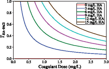end{document} changed as given in Fig. 5. According to Equation (13), the maximum number of HA macromolecules with a diameter of 75 nm that will fit on a PACl precipitate particle of 90 nm diameter when fully coating it is ∼6. The model predicted complete coverage of the PACl nanoparticles by HA for low PACl concentrations that correlated with very low observed turbidity removal efficiency.

OPEN IN VIEWER

FIG. 5.

Coverage of coagulant surface by HA as a function of coagulant dose.

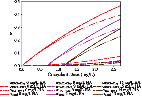
The relationships between the three terms included in attachment efficiency are given in Fig. 6. The term corresponding to collisions between a clean coagulant nanoparticle surface and clay \documentclass{aastex}\usepackage{amsbsy}\usepackage{amsfonts}\usepackage{amssymb}\usepackage{bm}\usepackage{mathrsfs}\usepackage{pifont}\usepackage{stmaryrd}\usepackage{textcomp}\usepackage{portland, xspace}\usepackage{amsmath, amsxtra}\usepackage{upgreek}\pagestyle{empty}\DeclareMathSizes{10}{9}{7}{6}\begin{document} $$\left( {{{ \bar \alpha }_{{ \rm{PACl}} - { \rm{Clay}}}}} \right)$$ \end{document} was always dominant for the experimental conditions in this dataset, and the other terms became relatively more important but still small with respect to \documentclass{aastex}\usepackage{amsbsy}\usepackage{amsfonts}\usepackage{amssymb}\usepackage{bm}\usepackage{mathrsfs}\usepackage{pifont}\usepackage{stmaryrd}\usepackage{textcomp}\usepackage{portland, xspace}\usepackage{amsmath, amsxtra}\usepackage{upgreek}\pagestyle{empty}\DeclareMathSizes{10}{9}{7}{6}\begin{document} $${\bar \alpha _{{ \rm{PACl}} - { \rm{Clay}}}}$$ \end{document} with increasing coagulant dose.

OPEN IN VIEWER

FIG. 6.

Attachment efficiency as a function of coagulant dose.

The model was validated by using it to predict turbidity removal efficiency for different experimental conditions. The predicted pC* and the measured pC* are compared in Fig. 7 for an additional 60 experiments with inflow turbidity of 100 NTU, PACl doses ranging from 0.53 to 2.65 mg/L as Al, and HA concentration ranging from 0 to 15 mg/L. The prediction is almost as good as for the 50 NTU data, with pC* RMSE of 0.11.

OPEN IN VIEWER

FIG. 7.

Comparison graph between predicted data and observed data for 100 NTU influent turbidity.

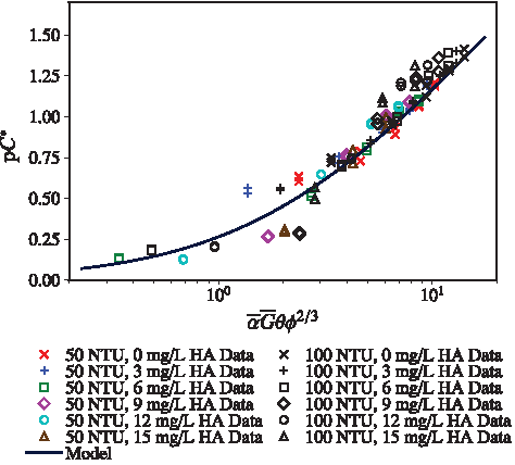
When the coagulant dose in Figs. 4 and 7 was replaced with the dimensionless group \documentclass{aastex}\usepackage{amsbsy}\usepackage{amsfonts}\usepackage{amssymb}\usepackage{bm}\usepackage{mathrsfs}\usepackage{pifont}\usepackage{stmaryrd}\usepackage{textcomp}\usepackage{portland, xspace}\usepackage{amsmath, amsxtra}\usepackage{upgreek}\pagestyle{empty}\DeclareMathSizes{10}{9}{7}{6}\begin{document} $$\overline { \alpha } \overline { G } \theta { \phi ^ { \frac { 2 } { 3 } } } $$ \end{document} , the data collapsed to a much narrower band, implying that the composite parameter, \documentclass{aastex}\usepackage{amsbsy}\usepackage{amsfonts}\usepackage{amssymb}\usepackage{bm}\usepackage{mathrsfs}\usepackage{pifont}\usepackage{stmaryrd}\usepackage{textcomp}\usepackage{portland, xspace}\usepackage{amsmath, amsxtra}\usepackage{upgreek}\pagestyle{empty}\DeclareMathSizes{10}{9}{7}{6}\begin{document} $$\overline { \alpha } \overline { G } \theta { \phi ^ { \frac { 2 } { 3 } } } $$ \end{document} , captures most of the trends present in the data, as given in Fig. 8.

OPEN IN VIEWER

FIG. 8.

Model fit of 50 and 100 NTU data for \documentclass{aastex}\usepackage{amsbsy}\usepackage{amsfonts}\usepackage{amssymb}\usepackage{bm}\usepackage{mathrsfs}\usepackage{pifont}\usepackage{stmaryrd}\usepackage{textcomp}\usepackage{portland, xspace}\usepackage{amsmath, amsxtra}\usepackage{upgreek}\pagestyle{empty}\DeclareMathSizes{10}{9}{7}{6}\begin{document} $${ \rm{p}}{C^*}$$ \end{document} as a function of effective collision potential. The data plotted include two replicates for each experiment.

In summary, the laminar-flow hydraulic flocculation model of Pennock et al. (2018) was modified to incorporate the effects of HA with the addition of a single-fitting parameter: a characteristic dimension of the HA macromolecules. The required coagulant dose can be predicted based on the flocculator parameters, HA characteristic size and concentration, and influent turbidity. The addition of HA to the flocculation model increases the model applicability because natural organic matter is found in all surface and ground waters and influences the coagulant dose needed for effective turbidity removal.

Discussion

For the range of experimental conditions considered in the research, the observed influence of HA on flocculation performance could be explained by the fractional coverage of the coagulant nanoparticle surfaces by HA, which, in turn, affected the fractional coverage of the suspended clay surfaces by coagulant. It is noteworthy that under the experimental conditions, the predictive success of the model was achieved without incorporating the charges of colloids, coagulant, and HAs. The reader is cautioned that the observations and predictions were obtained with one test particle, one coagulant, and one form of DOM in the mixed electrolyte represented by aerated, activated carbon-treated Cornell tap water, kept within the narrow pH range where coagulant precipitation is very favorable. While the experimental pH favored PACl precipitation, pH-dependent PACl solubility is accounted for in the model with \documentclass{aastex}\usepackage{amsbsy}\usepackage{amsfonts}\usepackage{amssymb}\usepackage{bm}\usepackage{mathrsfs}\usepackage{pifont}\usepackage{stmaryrd}\usepackage{textcomp}\usepackage{portland, xspace}\usepackage{amsmath, amsxtra}\usepackage{upgreek}\pagestyle{empty}\DeclareMathSizes{10}{9}{7}{6}\begin{document} \begin{align*} {{ N_ { { \rm { perClay } }}}} = { \frac { \left[ { { C_ { { \rm { PACl } } } } - { C_ { { \rm { PACl \; } } \left( { { \rm { aq } } } \right) } } } \right] { V_ { \rm { P } } } { \rho _ { \rm { P } } } } { \frac { \pi } { 6 } d_ { { \rm { PACl } } } ^3 { \rho _ { { \rm { PACl } } } } { C_0 } } } , \tag {18} \end{align*} \end{document}

where N_perClay is the number of precipitated coagulant aggregates per clay particle, C_PACl(aq) is the fraction of the coagulant dose that has remained in solution after precipitation using the PACl solubility observed by Van Benschoten and Edzwald (1990), and V_P is the volume of a single clay platelet (Swetland et al., 2014). Within the model, N_perClay is used to calculate \documentclass{aastex}\usepackage{amsbsy}\usepackage{amsfonts}\usepackage{amssymb}\usepackage{bm}\usepackage{mathrsfs}\usepackage{pifont}\usepackage{stmaryrd}\usepackage{textcomp}\usepackage{portland, xspace}\usepackage{amsmath, amsxtra}\usepackage{upgreek}\pagestyle{empty}\DeclareMathSizes{10}{9}{7}{6}\begin{document} $$\bar \alpha$$ \end{document} , as it is a component of the calculation for \documentclass{aastex}\usepackage{amsbsy}\usepackage{amsfonts}\usepackage{amssymb}\usepackage{bm}\usepackage{mathrsfs}\usepackage{pifont}\usepackage{stmaryrd}\usepackage{textcomp}\usepackage{portland, xspace}\usepackage{amsmath, amsxtra}\usepackage{upgreek}\pagestyle{empty}\DeclareMathSizes{10}{9}{7}{6}\begin{document} $${{ \rm{ \overline \Gamma }}_{{ \rm{PACl}} - { \rm{Clay}}}}$$ \end{document} : \documentclass{aastex}\usepackage{amsbsy}\usepackage{amsfonts}\usepackage{amssymb}\usepackage{bm}\usepackage{mathrsfs}\usepackage{pifont}\usepackage{stmaryrd}\usepackage{textcomp}\usepackage{portland, xspace}\usepackage{amsmath, amsxtra}\usepackage{upgreek}\pagestyle{empty}\DeclareMathSizes{10}{9}{7}{6}\begin{document} \begin{align*} {{{ \overline \Gamma}}} _ { { \rm { PACl }} - { \rm { Clay } } } = 1 - { e^ { - { \frac { d_ {{\rm { PACl}}} ^2 } { { \rm { S } } { { \rm { A } } _ { { \rm { Clay } } } } } } \; { N_ { { \rm { perClay } } } } { R_ { { \rm { Clay } } } } \; } } , \tag { 19 } \end{align*} \end{document}

where SA_Clay is the surface area of the suspended clay particles and R_Clay is the fraction of the available surface area in the reactor (including the surface area of reactor walls) that belongs to suspended clay particles (Swetland et al., 2014).

The solubility of HA also is highly pH dependent, and additional experimental results are needed to test the applicability of the model approach as a function of varying pH. The experimental conditions were designed to keep the pH relatively constant, and the pH change in the experiments was small (7.5 ± 0.3). As the presence of DOM acts as a precursor for the formation of residual byproducts, pH-dependent removal of DOM by coagulation and flocculation is of great interest and is a planned topic for future research.

The model considered flocculation in the presence of HA as a two-step process. First, HA macromolecules attached to precipitated coagulant nanoparticles. Then, the partially coated coagulant nanoaggregates could bind to clay and reactor wall surfaces. HA and coagulant nanoparticles were treated as spheres when estimating the attachment efficiency based on surface coverage and probability. The diameter of precipitated PACl nanoparticles was experimentally measured to be 90 nm by Garland (2017), and an HA macromolecule diameter of 75 nm best fit the observations. Wall loss of coagulant precipitates with HA nanoaggregates was considered, whereas direct wall loss of HA macromolecules was not considered.

The characteristic HA dimension, d_HA, has physical relevance, with the fitted value, 75 nm, falling within the range (4–110 nm) reported by Österberg et al. (1993), and the model fits are well correlated to the observations. The predictive capability of the model was verified by predicting results under different experimental conditions with no additional adjustable parameters.

The flocculation model without the effects of HA shows that pC* is directly proportional to the log of the effective collision potential, \documentclass{aastex}\usepackage{amsbsy}\usepackage{amsfonts}\usepackage{amssymb}\usepackage{bm}\usepackage{mathrsfs}\usepackage{pifont}\usepackage{stmaryrd}\usepackage{textcomp}\usepackage{portland, xspace}\usepackage{amsmath, amsxtra}\usepackage{upgreek}\pagestyle{empty}\DeclareMathSizes{10}{9}{7}{6}\begin{document} $$ { \rm { log } } \left( { \overline { \alpha } \overline { G } \theta { \phi ^ { \frac { 2 } { 3 } } } } \right)$$ \end{document} , and this relationship is still present in the model with a modified attachment efficiency, \documentclass{aastex}\usepackage{amsbsy}\usepackage{amsfonts}\usepackage{amssymb}\usepackage{bm}\usepackage{mathrsfs}\usepackage{pifont}\usepackage{stmaryrd}\usepackage{textcomp}\usepackage{portland, xspace}\usepackage{amsmath, amsxtra}\usepackage{upgreek}\pagestyle{empty}\DeclareMathSizes{10}{9}{7}{6}\begin{document} $$\bar \alpha$$ \end{document} , based on clay surface coverage by coagulant nanoparticles as adjusted for the presence of HAs.

Under experimental conditions, the modified flocculation model provides the fundamental basis for the relationship between coagulant dose, synthetic raw water clay, and HA concentrations. Extension to natural waters will undoubtedly require additional research.

The form of the flocculation model equation sets the interactions between raw water properties (φ₀), influent particle surface area (that contributes to \documentclass{aastex}\usepackage{amsbsy}\usepackage{amsfonts}\usepackage{amssymb}\usepackage{bm}\usepackage{mathrsfs}\usepackage{pifont}\usepackage{stmaryrd}\usepackage{textcomp}\usepackage{portland, xspace}\usepackage{amsmath, amsxtra}\usepackage{upgreek}\pagestyle{empty}\DeclareMathSizes{10}{9}{7}{6}\begin{document} $$\;{{ \rm{ \overline \Gamma }}_{{ \rm{PACl}} - { \rm{Clay}}}}$$ \end{document} ), coagulant precipitate size and dose (that contributes to \documentclass{aastex}\usepackage{amsbsy}\usepackage{amsfonts}\usepackage{amssymb}\usepackage{bm}\usepackage{mathrsfs}\usepackage{pifont}\usepackage{stmaryrd}\usepackage{textcomp}\usepackage{portland, xspace}\usepackage{amsmath, amsxtra}\usepackage{upgreek}\pagestyle{empty}\DeclareMathSizes{10}{9}{7}{6}\begin{document} $${{ \rm{ \overline \Gamma }}_{{ \rm{PACl}} - { \rm{Clay}}}}$$ \end{document} and \documentclass{aastex}\usepackage{amsbsy}\usepackage{amsfonts}\usepackage{amssymb}\usepackage{bm}\usepackage{mathrsfs}\usepackage{pifont}\usepackage{stmaryrd}\usepackage{textcomp}\usepackage{portland, xspace}\usepackage{amsmath, amsxtra}\usepackage{upgreek}\pagestyle{empty}\DeclareMathSizes{10}{9}{7}{6}\begin{document} $${{ \rm{ \overline \Gamma }}_{{ \rm{HA}} - { \rm{PACl}}}}$$ \end{document} ), HA molecule size and concentration (that contributes to \documentclass{aastex}\usepackage{amsbsy}\usepackage{amsfonts}\usepackage{amssymb}\usepackage{bm}\usepackage{mathrsfs}\usepackage{pifont}\usepackage{stmaryrd}\usepackage{textcomp}\usepackage{portland, xspace}\usepackage{amsmath, amsxtra}\usepackage{upgreek}\pagestyle{empty}\DeclareMathSizes{10}{9}{7}{6}\begin{document} $${{ \rm{ \overline \Gamma }}_{{ \rm{HA}} - { \rm{PACl}}}}$$ \end{document} ), flocculator design \documentclass{aastex}\usepackage{amsbsy}\usepackage{amsfonts}\usepackage{amssymb}\usepackage{bm}\usepackage{mathrsfs}\usepackage{pifont}\usepackage{stmaryrd}\usepackage{textcomp}\usepackage{portland, xspace}\usepackage{amsmath, amsxtra}\usepackage{upgreek}\pagestyle{empty}\DeclareMathSizes{10}{9}{7}{6}\begin{document} $$\left( { \overline G \theta } \right)$$ \end{document} , and sedimentation tank design (k). An increase in concentration of HA causes an increase in \documentclass{aastex}\usepackage{amsbsy}\usepackage{amsfonts}\usepackage{amssymb}\usepackage{bm}\usepackage{mathrsfs}\usepackage{pifont}\usepackage{stmaryrd}\usepackage{textcomp}\usepackage{portland, xspace}\usepackage{amsmath, amsxtra}\usepackage{upgreek}\pagestyle{empty}\DeclareMathSizes{10}{9}{7}{6}\begin{document} $${{ \rm{ \overline \Gamma }}_{{ \rm{HA}} - { \rm{PACl}}}}$$ \end{document} , which decreases pC* but can be compensated for by increasing coagulant dose to increase \documentclass{aastex}\usepackage{amsbsy}\usepackage{amsfonts}\usepackage{amssymb}\usepackage{bm}\usepackage{mathrsfs}\usepackage{pifont}\usepackage{stmaryrd}\usepackage{textcomp}\usepackage{portland, xspace}\usepackage{amsmath, amsxtra}\usepackage{upgreek}\pagestyle{empty}\DeclareMathSizes{10}{9}{7}{6}\begin{document} $${{ \rm{ \overline \Gamma }}_{{ \rm{PACl}} - { \rm{Clay}}}}$$ \end{document} .

Summary

The development of a predictive model for laminar-flow hydraulic flocculation of water containing clay and HA is described. The study results increase the flexibility and generality of the AguaClara hydraulic flocculation model, and the modified model provides insight into the mechanism by which HA causes a decrease in performance of coupled flocculation–sedimentation processes.

The model was able to predict independent experimental results for a different raw water turbidity with no additional adjustable parameters and represents a new approach to account for the effect of DOM on flocculation of inorganic particulate matter. Further tests should be carried out to fully validate the laminar-flow model including consideration of different experimental surrogates for DOM, different colloidal surfaces, alternative coagulants, and varying solution compositions, including pH.