Response Surface Modeling and Setpoint Determination of Steam- and Air-Assisted Flares

Abstract

Federal Regulation 40 CFR §63.670 requires flare operators to specify smokeless design capacity for flares with no visible emissions. Alternatively, 96.5% combustion efficiency (CE) or 98% destruction efficiency must be achieved with threshold limits of minimum combustion zone net heating value (NHV_cz) ≥ 270 British thermal unit/standard cubic feet (BTU/scf) for steam-assisted and net heating value dilution parameter (NHV_dil) ≥ 22 BTU/ft² for air-assisted flares. There is still no guarantee for smokeless flaring (SLF) or CE >96.5%. Robust response surface models developed in this study expressed %CE and %Opacity as a function of operating variables for air- and steam-assisted flares. Opacity and CE test data from 1983 to 2016 were analyzed. General quadratic models with transforms of CE and Opacity showed R² > 0.90, and bivariate sigmoid models for CE showed R² > 0.87. Two-dimensional (2D) contours illustrate the trends of major operating parameters. Operational setpoints at the incipient smoke point (ISP) and SLF were determined by solving the models subject to NHV_cz and NHV_dil threshold limits specifying Opacity at 3% (ISP) and 2% (SLF). The predicted steam/air assists/makeup fuel, NHV_cz (or NHV_dil), and CE at ISP and SLF conditions are compared with the experimental 1984 Environmental Protection Agency (EPA) and 2010 Texas Commission on Environmental Quality flare study ISP test data. These setpoints would help flare operators to establish ISP or SLF conditions either by adding makeup fuel to vent gas with low heating value or by minimizing the assist without adding makeup fuel for steam- and air-assisted flares.

Introduction

Flares are an important safety device for pressure relief from process units and storage vessels, especially during start-up, shutdown, and malfunction situations. Flares dispose of purged and waste products from refineries, gaseous wastes from chemical processing, vent gases from furnaces and coke ovens, and unrecoverable gases from oil/gas industries (U.S. EPA, 2018b). Russia leads the top 30 flaring countries (19.9 billion cubic meters [bcm] in 2017), while the United States ranks fourth, flaring 9.5 bcm in 2017 according to World Bank satellite data (Korppoo, 2018; World Bank, 2018). Flare emissions consist of unburned fuel (methane and unburned volatile organic compounds) and combustion byproducts such as soot, CO, CO₂, oxides of nitrogen, and sulfur (Singh et al., 2014a). These emissions have direct health impacts associated with exposure and indirect health impacts like the resulting ozone formation. For instance, flares account for 61% of the highly reactive volatile organic compounds (HRVOCs) emissions based on the 2007 HRVOC special emissions inventory data collected from the projects undertaken by the facilities in Harris County, Texas (ENVIRON, 2008, 2009).

Flaring can also emit black carbon (BC) as a by-product, which is an anthropogenic forcer of climate with public health implications (Anenberg et al., 2012; Bond et al., 2013; Stohl et al., 2013; Schwartz et al., 2015). Gas flaring dominates the estimated BC emissions in the Arctic, while it contributes to 3% of global BC emissions (Stohl et al., 2013). During its short life time for a few days, 1 g of BC warms the atmosphere several hundred times >1 g of CO₂ does in 100 years (Jacobson et al., 2013). Control of BC and VOC emissions from flaring is an important issue from the environmental standpoint.

Destruction efficiency (DE) and combustion efficiency (CE) are common indicators of flare performance in addition to smoke generated by incomplete combustion of hydrocarbons (Schwartz et al., 2001; U.S. EPA, 2012).

Federal regulations (40CFR60.18 and 63.670) require smokeless flaring (SLF), which motivates flare operators to oversteam or overair to suppress smoke at the expense of CE. Recently, Environmental Protection Agency (EPA), in addition to combustion zone net heating value (NHV_cz) requirements, required steam-assisted flares with the perimeter assist air intentionally entrained in lower and upper steam at the flare tip of diameter <9 in. needs to meet net heating value dilution parameter (NHV_dil) ≥ 22 BTU/ft². Flare operators should establish the smokeless capacity in a 15-min block average to ensure 98% DE or 96.5% CE or higher at all times, and assess the exceedance of the smokeless capacity based on cumulative volumetric flow rate and/or flare tip velocity (U.S. EPA, 2018a). Still, there is no guarantee that CE will be ≥96.5% (Fry and Coburn, 2012; Zeng et al., 2016).

Furthermore, many operation parameters such as steam assist (S) and air assist (A) used to combust vent gas, flare tip exit velocity (V), vent gas composition (carbon to hydrogen molar ratio [CHR]), net heating value (NHV), flare tip diameter (D), and wind speed (u) affect flare performance by influencing soot formation and unburned VOC emissions (Castiñeira and Edgar, 2006; Allen and Torres, 2011a, 2011b; Levitsky, 2011). All these issues lead to questions of operating flares in a most environmentally responsible and cost-effective manner in compliance with regulations, achieving SLF, and still maximizing CE under a given set of design and operating conditions.

Few studies were performed to predict flare emissions and performance using computational fluid dynamics (CFD) and WRF-SMOKE-CMAQ modeling system (Singh et al., 2012, 2014a, 2014b; Pan et al., 2015; Damodara et al., 2017). Field measurements (such as FTIR, MEMS, EI, LIF, and REMPI) for estimating flare efficiency are expensive and difficult to deploy on-site, even though the remote, optical CE measurement technology developed by Providence Photonics (Zeng et al., 2016) has gained much attention. Detailed CFD flare modeling based on rigorous kinetic mechanisms is also comparatively expensive and time-consuming. As a result, this study seeks to develop easy-to-use response surface models in quadratic form and sigmoid functions to predict the flare performance in terms of operational parameters based on the experimental study with soot and CE data. Quadratic form is the highest order linear regression in response surface methodology apt to model a curved relationship between input variables and the responses.

Similarly, sigmoid function is a nonlinear regression used to model curve relationships, and mathematically explain relation between a response and one or more predictor variables. Both functions can yield graphs to show curvatures (Minitab, 2018). Logit functions of response variables showed better data distribution and more accurate fitting. Bivariate sigmoid functions are developed with major parameters NHV_cz (or NHV_dil) and V per 40 CFR 63.670 requirements for flares. Two-dimensional contours illustrate the trends of major operating parameters.

Large and varying time delays in gas chromatograph (GC) analysis (15–20 min) in vent gas heating value measurements, nonlinear behavior of flaring process with wide variation in waste gas stream flow, and use of N₂ as a purge gas to maintain positive pressure in the vent gas pipes were the major challenges in flaring control. Model-Free Adaptive control (Cybosoft, 2016) and steam to hydrocarbon ratio control with feed-forward action minimized the time delays caused by GC analysis and overcame those challenges with robust performance (Srinivasarao and Krishna, 2015, 2017).

Since various parameters affect the flare performance, simple guidelines for SLF were elusive (ENVIRON, 2009; U.S. EPA, 2009, 2015). Therefore, setpoints to adjust steam/air or makeup fuel in a feed-forward control based on a prediction model to ensure smokeless combustion are critical. The second objective of this study is to determine the operation setpoints for S (or A) and makeup fuel volumetric flow rate ( ${Q'}_{f}$ ) at the incipient smoke point (ISP) and SLF by solving the response surface models, specifying NHV_cz ≥ 270 BTU/standard cubic feet (scf) and NHV_dil ≥ 22 BTU/ft² per EPA's finalized maximum achievable control technology rules for refineries. This study considers natural gas as the makeup fuel with a heating value of 980 BTU/scf.

Methodology

Data source and analysis

The experimental data for response surface models collected from previous flare study reports include flare efficiency study (McDaniel, 1983), evaluation of the efficiency of industrial flares (Pohl et al., 1984), 2010 Texas Commission on Environmental Quality (TCEQ) flare study final report (Allen and Torres, 2011a, 2011b), Marathon Petroleum company flare study report (Cade and Evans, 2010; Roesler et al., 2010), Carleton University soot emission rate measurements (Corbin and Johnson, 2014a, 2014b), and Providence Photonics data (Zeng et al., 2016). Data collected from the literature include the geometry of steam-, air-, and nonassisted flares, meteorological data (crosswind speed/direction), operating data (aeration, steaming, exit velocity, waste gas/pilot fuel species), flare efficiencies, and soot emission.

Table 1 shows the data sources and the range of the variables used in response surface models. Since the flare tests conducted include different fuel mixtures such as propylene, propane, natural gas, methane, ethylene, and typical refinery fuel, the presence of π-bond (Pi_vg) in vent gas, π-bond in the combustibles (Pi_cz), carbon number (CN) and CHR of vent gas were introduced to account for the effect of vent gas composition. The presence of π-bonds is highly correlated with the SP² hybridization of carbon atoms, which increases the absorption efficiency of carbon when it cools down due to large number of free charge careers resulting in higher electron density caused by π-bonds (Jager et al., 1999). Alkenes with higher CHR have π-bonds, which are highly correlated with SP² hybridization of carbon atoms, which may lead to higher Opacity as absorption efficiency increases due to high electron density. π-Bonds and σ-Bonds section in Supplementary Data (as shown in Supplementary Fig. S1) discuss π-bond and its presence in different molecules and compounds.

Table 1.

Data Sources used in Response Surface Models

Flare study	Year	Assist	Vent gas mixture	No. of data points
McDaniel	1983	Air	Propylene and N₂	1
McDaniel	1983	Steam	Propylene and N₂	2
Pohl, Payne, and Lee	1984	Steam	Propane and N₂	58
TCEQ	2010	Air	100% Propylene, Propylene/TNG and N₂	56
		Air	Propane/TNG and N₂	56
		Steam	100% Propylene, Propylene/TNG and N₂	70
		Steam	Propane/TNG and N₂	70
MPC—TX	2010	Steam	Typical refinery fuel	44
MPC—Detroit	2010	Steam	Typical refinery fuel	56
Carleton University	2014	Nonassist	Average 6-mix	14
			Heavy 4-mix	15
			100% Ethylene	4
Providence Photonics	2016	Air	100% Propane	12
Providence Photonics	2016	Steam	100% Propylene and 100% propane	17

TCEQ, Texas Commission on Environmental Quality; TNG, Tulsa natural gas.

Flare data include a wide range of diameters 1.5–3 in. for laboratory-scale flares and 3–36 in. for industrial flares. Only two of R, u, and V are selected interchangeably as the independent variables to analyze their effect on the response variables. In other words, R and u represent two degrees of freedom as u and V. Models developed including R in conjunction with u help us analyze the effect of V at a constant u. Modeling trials showed CE models developed with R and u and Opacity models developed with u and V predicted better with high R² values. Variable transform methods such as logit and log functions showed better distributions for CE and Opacity (Supplementary Fig. S2). Therefore, air-assisted flare models were developed with Logit (100–CE) and Logit Opacity as the response variables. Since Absorbance (Abs) is equivalent to 2–log (100–Opacity) (Gallik, 2017), steam-assisted flare models were developed with Logit (100–CE) and Log Abs as the response variables.

CE reported in 2010 TCEQ flare study report (Allen and Torres, 2011a, 2011b) were corrected for soot emissions to a maximum of 0.2% based on revised data provided by Aerodyne Research, Inc. (Aerodyne Research Inc, 2010; Fortner et al., 2012). To develop the precise model equations, CE was recalculated considering the soot emissions as expressed in the following equation: $\begin{matrix} C E = & [C O_{2 p l u m e} ∕ (C O_{2 p l u m e} + C O_{p l u m e} + Σ H C_{p l u m e} + s o o t)] \\ \times 100, \end{matrix}$ (1)

where soot is the volume concentration of BC particles (molecular weight [MW] = 12.01) in the plume (parts per million by volume, ppmv) after combustion has ceased.

According to Allen and Torres (2011a, 2011b), NHV_cz is defined as $\begin{matrix} N H V_{c z} = & ({Q'}_{v g} * N H V_{v g} + {Q'}_{p g} * N H V_{p g}) ∕ \\ ({Q'}_{v g} + {Q'}_{s} + {Q'}_{p g}), \end{matrix}$ (2)

where ${Q'}_{v g}$ is the volumetric flow rate of vent gas (scf/h), ${Q'}_{p g}$ is the volumetric flow rate of pilot gas (scf/h), NHV_pg is the net heating value of pilot gas (BTU/scf), and ${Q'}_{s}$ is the volumetric flow rate of assisted steam (scf/h).

NHV_dil is defined by U.S. EPA (2015) as $N H V_{d i l} = ({Q'}_{v g} * N H V_{v g} * D) ∕ ({Q'}_{v g} + {Q'}_{s} + {Q'}_{A}),$ (3)

where NHV_dil is the net heating value dilution parameter (BTU/ft²) and ${Q^{'}}_{A}$ is the volumetric flow rate of assisted air (scf/h).

General quadratic response surface modeling

Generalized response surface models were established using Minitab 18 statistics toolbox (Minitab, 2018). Initially, a linear model is developed, and then the model is validated based on R², adjusted R², predicted R², and analysis of variance table to check the adequacy of each parameter for the response (Ma et al., 2015). The significance of the coefficients in the model was determined based on p-value (Homayoonfal et al., 2015). If a linear model is not appropriate, then a quadratic model is developed to show the curvature in response surface (Minitab, 2018). The interaction terms with significant effects were added to the model for better fitting by the stepwise regression option in Minitab while performing response surface analysis. Outliers were removed in each step based on standardized residual plot analysis, and then recursive regression was performed to develop the final model (Model Validation section, Best Subsets Regression: Logit (%Opacity) Versus A, CHR, D, V, u, NHV_dil, section as shown in Supplementary Table S1, Removal of Outliers section, and Validation of the Model Logit (100–%CE) Versus A, CHR, D, R, NHV_dil section in Supplementary Data as shown in Supplementary Fig. S3).

The quadratic form of the response surface model is expressed as $Z = a_{0} + Σ_{i} a_{i} X_{i} + Σ_{i} a_{i i} {X_{i}}^{2} + Σ_{i} Σ_{j} b_{i j} X_{i} X_{j} + e,$ (4)

where Z is the response variable, X is the operational variable, i = 1 to n (n—the number of variables), e is the residual error, a₀ is the constant term, a_i are the linear coefficients, a_ii are the quadratic coefficients, and b_ij are the interaction coefficients. The coefficients were determined by solving the regression equation using the experimental values of operational variables, so that the residual error is minimized. 80% of the data were randomly selected using Excel for model development, and the remaining 20% data were used for model validation, such that the data used in model validation lie within the range of the variables used in models. VE (variance explained, %) and MAE (mean absolute error, %) (Li, 2017) are reported as accuracy and error measures for the Opacity and CE back-calculated from the response variables (Accuracy and Error Measures section in Supplementary Data).

Statistically significant and highly correlated variables determined by Best Subsets Regression method are V, u, A, NHV_dil, D, and CHR for Logit Opacity and A, CHR, NHV_dil, and R for Logit (100–CE) models for air-assisted flares. CHR, CN, NHV_cz, S, V, and u were found to have a significant effect on Log (Abs), while CHR, CN, NHV_cz, R, S, and u had a significant effect on Logit (100–CE) for steam-assisted flares.

Sigmoid models

Sigmoid function is a nonlinear function that fits the data, which do not exhibit general linear behavior (Bates and Watts, 1988; Bates and Chambers, 1992; Fox, 2008; Smith, 2012). This function forms an “S” shape (sigmoid curve) and is expressed as $S (t) = 1 ∕ (1 + e^{- t}) .$ (5)

Equation (5) is modified by introducing a coefficient “a” to the exponent “e” and substituting NHV_cz (combustion zone parameter) for t, and then CE is expressed as $C E = 100 ∕ (1 + a * e^{- b * N H V c z}) .$ (6)

CE exhibited an “S” shape characteristic of the sigmoid function when plotted against NHV_cz in a previous study (Smith, 2012). Parameters a and b were estimated using the curve fitting toolbox of MATLAB (Mathworks, 2015). As the numerical methods used in these algorithms are sensitive to initial guess, a proper initial guess is critical for better prediction (Galant, 1975; Ratkowsky, 1990). Initial guess was estimated by minimizing the errors using Excel Solver.

Bivariate model for CE was developed with NHV_cz and flare tip exit velocity as the independent variables for the data range shown in Table 2. The coefficient of NHV_cz in Equation (6) has been parameterized to become a linear function of V (promotes fuel-air mixing) to adjust for the slope change of the sigmoid function at the inflection point due to V. The location of the inflection point is also parameterized as d+e * V, and the bivariate sigmoid function is expressed as follows:

Table 2.

Steam-Assisted Flare Test Data Ranges Used in Response Surface Models

%Opacity	%CE	Pi_vg (mol ⁻ ¹)	CHR	NHV_cz (BTU/scf)	CN	S (lb/MMBTU)	V (ft/s)
0.01–99.9	16.3–99.9	0–1.79	0.2–0.5	90–2316	0.37–3.08	0–514	0.2–428

Source: Data are from references (McDaniel, 1983; Pohl et al., 1984; Aerodyne Research Inc., 2010; Cade and Evans, 2010; Roesler et al., 2010; Allen and Torres, 2011a, 2011b; Fortner et al., 2012; Corbin and Johnson, 2014a, 2014b; Zeng et al., 2016).

BTU, British thermal unit; CE, combustion efficiency; CHR, carbon to hydrogen molar ratio; CN, carbon number; NHV_cz, combustion zone net heating value; scf, standard cubic feet.

C E = 100 ∕ (1 + a * e^{((b + c * V) * (N H V c z - (d + e * V)))}) .

(7)

Finally, Equation (8) is derived by multiplying the two components of the exponent “e” in Equation (7), and the simplified quadratic function is expressed as $C E = 100 ∕ (1 + a * e^{(b * N H V c z - c * V + d * N H V c z * V - e * V^{\land} 2)}) .$ (8)

In a similar method, univariate and bivariate sigmoid models for CE were developed involving NHV_dil and V for air-assisted flares.

Setpoint determination of operation variables

Response surface models for Opacity are solved by equating the models to 3% (ISP) and 2% (SLF) based on the ISP characterization (Chen and Alphones, 2019) using the Newton-Raphson method in Polymath to determine the setpoints for steam (or air assist) and makeup fuel specifying NHV_cz ≥ 270 BTU/scf for steam-assisted or NHV_dil ≥ 22 BTU/ft² for air-assisted flares. The initial values are chosen to solve the Opacity models for the minimum steam (or air assist) with minimum makeup fuel flow rate ( ${Q'}_{f} = 0$ ). For cases with low NHV_dil or NHV_cz requiring makeup fuel ( ${Q'}_{f}$ ) to meet the threshold limits, the makeup fuel flow rate is added to NHV_vg to redefine NHV_vg as shown in Equation (9). NHV_vg is replaced by NHV_vg,req in the CE and Opacity models. Setpoints for A (or S) and ${Q'}_{f}$ determined from the Opacity models were then substituted in CE models to solve for predicted CE values. $N H V_{v g, r e q} = (N H V_{v g} * {Q'}_{v g} + N H V_{f} * {Q'}_{f}) ∕ ({Q'}_{v g} + {Q'}_{f}) .$ (9)

Setpoint determination for steam-assisted flares

O p a c i t y = g (N H V_{c z}, S)

(10)

N H V_{c z} = h (N H V_{v g, r e q}, {Q'}_{f}, S)

(11)

C E = f (N H V_{c z}, S)

(12)

Equations (10) and (11) were solved for S and NHV_cz by specifying makeup fuel flow rate, ${Q'}_{f} = 0$ , and Opacity = 3%. If the calculated NHV_cz < 270 BTU/scf, then makeup fuel ( ${Q'}_{f}$ ) is required to increase the NHV_vg, thereby increasing NHV_cz. In that case, S and ${Q'}_{f}$ were calculated by specifying NHV_cz = 270 BTU/scf and Opacity = 3%. The resulting setpoints were substituted in Equation (12) to find CE. The detailed procedure is shown in Fig. 1A. Setpoints for SLF condition are determined specifying Opacity as 2%, and the above procedure is repeated as shown in Fig. 1B.

FIG. 1.

(A) Flow chart for setpoint determination of ${Q'}_{f}$ , NHV_cz, and S for steam-assisted flares at ISP. (B) Flow chart for setpoint determination of ${Q'}_{f}$ , NHV_cz, and S for steam-assisted flares at SLF. CE, combustion efficiency; ISP, incipient smoke point; NHV_cz, combustion zone net heating value; SLF, smokeless flaring.

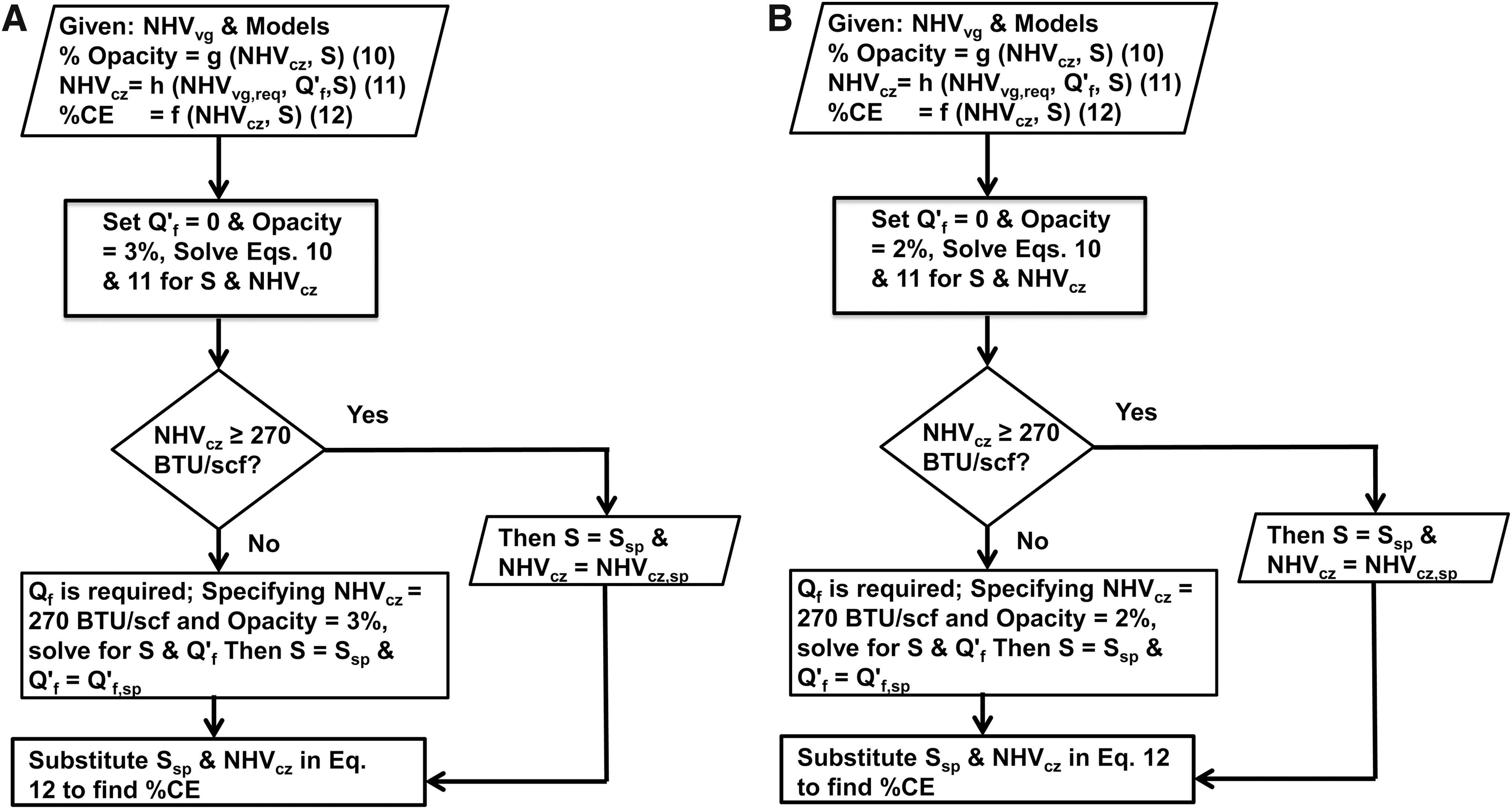
Setpoint determination for air-assisted flares

O p a c i t y = g (N H V_{d i l}, A)

(13)

N H V_{d i l} = h (N H V_{v g, r e q}, {Q'}_{f}, A)

(14)

C E = f (N H V_{d i l}, A)

(15)

Equations (13) and (14) were solved for A and NHV_dil by specifying ${Q'}_{f} = 0$ and Opacity = 3%. If the calculated NHV_dil < 22 BTU/ft², then ${Q'}_{f}$ is required to increase the vent gas heating value, thereby increasing the NHV_dil. Then by specifying NHV_dil = 22 BTU/scf and Opacity = 3%, A and ${Q'}_{f}$ were determined. The resulting setpoints were substituted in Equation (15) to find CE. The detailed procedure is shown in Fig. 2A. Opacity is specified at 2% for SLF conditions, and the setpoints are determined by the same procedure as shown in Fig. 2B.

FIG. 2.

(A) Flow chart for setpoint determination of ${Q'}_{f}$ , NHV_dil, and A for air-assisted flares at ISP. (B) Flow chart for setpoint determination of ${Q'}_{f}$ , NHV_dil, and A for air-assisted flares at SLF. NHV_dil, net heating value dilution parameter.

Results and Discussions

General quadratic response surface models

Response surface models for steam-assisted flares

Response surface models were developed for the transformed response variables Log Abs and Logit (100–CE) to fit the steam-assisted flare data range shown in Table 2. As the parameters representing vent gas species, CHR, and Pi_vg are highly correlated (Pearson's correlation coefficient >0.7), two sets of models were developed for Opacity and CE, one with CHR and other with Pi_vg. Table 3 shows the final models with N (number of data points), R², and R² _(Adj), including VE% and MAE% values for the back-calculated Opacity and CE. Based on the accuracy measure expressed as VE%, error measure expressed as MAE%, R², and number of terms, the best model was chosen for further analysis and setpoint determination.

Table 3.

General Quadratic Model Equations for Steam-Assisted Flares

Model equations	Model			%CE (%Opacity)
Model equations	N	R²	R²_(Adj)	MAE (%)	VE (%)
Logit (100–CE) = 0.237 − 7.06E-03 NHV_cz + 1.88 CN +1.6E-06 NHV_cz² − 8.7E-06 S² − 12.3 CHR² + 3.3E-03 R ^* u − 3.68E-04 R ^* S − 2.9E-05 u ^* NHV_cz − 6.6E-05 NHV_cz ^* S + 9.3E-03 NHV_cz ^* CHR −9.28E-04 NHV_cz ^* CN +0.054 S ^* CHR −6.77E-03 S ^* CN	203	0.93	0.92	2.1	90
Logit (100–CE) = −2.852 − 0.1825 R + 0.0173 u + 1.5E-04 NHV_cz + 0.0111 S + 0.4022 Pi_vg − 1.6E-05 S² + 0.0069 R ^* u + 2.9E-04 R ^* NHV_cz − 3.4E-05 u ^* NHV_cz − 0.0283 u ^* Pi_vg + 0.0029 S ^* Pi_vg	203	0.88	0.87	2.8	84
Log Abs = −2.36 − 2.4E-03 NHV_cz − 8.1E-03 S − 0.034 V + 0.0777 u + 1.67 CN +1.4E-05 S² + 4.4E-05 V² − 3.02 u² − 0.3774 CN² + 6.7E-05 NHV_cz ^* V + 3.5E-03 NHV_cz ^* CHR +6.6E-04 NHV_cz ^* CN +5.4E-04 S ^* V − 5.7E-03 S ^* CHR −2.4E-03 V ^* u − 0.039 V ^* CN	184	0.91	0.90	0.94	96
Log Abs = −2.46 − 0.0172 V + 0.0635 u − 1.76E-03 NHV_cz − 7.72E-03 S + 0.850 Pi_cz + 0.0516 MW +2.7E-05 V² − 0.0025 u² + 1.1E-05 S² − 0.0018 MW² − 0.0446 u ^* Pi_CZ + 8E-06 NHV_cz ^* S + 8.3E-05 NHV_cz ^* MW	184	0.90	0.89	1.1	93

Units and the data range for the models are provided in Table 1; R² and R²_(Adj) represent the correlation between experimental and predicted Logit functions, while MAE% and VE% are between the experimental and the predicted CE or Opacity.

MAE, mean absolute error; MW, molecular weight; VE, variance explained.

Figure 3 indicates good correlation between the experimental and predicted values for the Logit (100–CE) model. Table 4 shows the parameter estimates and their coefficients with 95% confidence interval and p-values for Logit (100–CE) model. The significance of the parameters was determined from their p-values <0.001 and standard error values smaller than the estimated coefficient values (Ghoreishian et al., 2016). Likewise, the parameters and their coefficients in Log Abs model were validated based on 95% confidence interval and p-values.

FIG. 3.

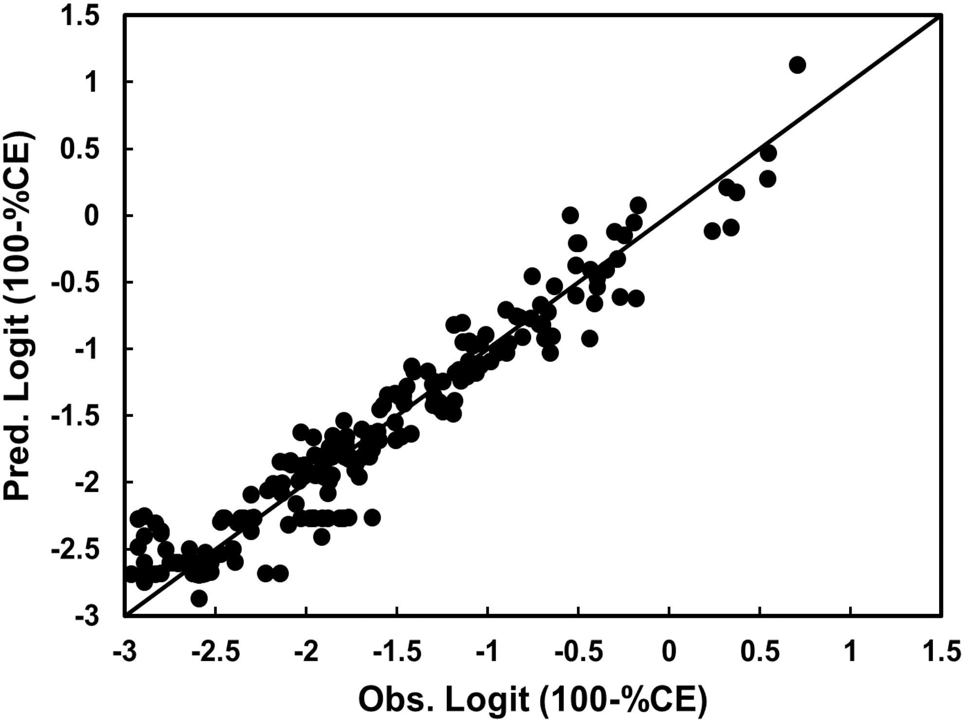
Comparison of experimental and predicted values of the Logit (100–CE) model for steam-assisted flares.

Table 4.

Coded Coefficients of the General Quadratic Model Logit (100–CE) for Steam-Assisted Flare Test Data

Variable	Coeff	SE Coeff	95% CI	p-Value
Constant	0.2370	0.2052	−0.1677 to 0.6418	0.249
NHV_cz	−7.1E-03	4.7E-04	−8E-03 to −6.1E-03	0.000
CN	1.8795	0.1906	1.503 to 2.255	0.000
NHV_cz²	1.6E-06	2.9E-07	1.1E-06 to 2.2E-06	0.000
S²	−8.7E-06	1.5E-06	−1.2E-05 to −5.8E-06	0.000
CHR²	−12.31	0.9692	−14.23 to −10.40	0.000
R ^* u	0.0033	4.5E-04	0.0024 to 0.0042	0.000
R ^* S	−3.7E-04	4.2E-05	−4.5E-04 to −2.9E-04	0.000
u ^* NHV_cz	−2.9E-05	5.1E-06	−3.9E-05 to −1.9E-05	0.000
NHV_cz ^* S	−6.6E-05	5.7E-06	−7.7E-05 to −5.5E-05	0.000
NHV_cz ^* CHR	9.3E-03	7.1E-04	7.9E-03 to 0.0107	0.000
NHV_cz ^* CN	−9.3E-04	1.8E-04	−0.0013 to −5.7E-04	0.000
S ^* CHR	0.0538	2.8E-03	0.0482 to 0.0593	0.000
S ^* CN	−6.8E-03	8.2E-04	−0.0084 to −0.0053	0.000

CI, confidence interval; SE, standard error.

Effect of operating parameters on Opacity and CE for steam-assisted flares

The effect of major parameters on the predicted Opacity from the Log Abs model was illustrated by 2D contour plots, while other parameters were fixed at certain values. Figure 4A and B show the 2D contour plot for predicted Opacity versus NHV_cz, V at two different levels of CHR (0.38 for 100% propane and 0.43 for propylene and Tulsa natural gas [TNG] mixture), while S, u, and CN are fixed. The contour lines in the 2D plots are intended to show the effect of the operating parameters based on proposed models, while the black dots represent the experimental data.

FIG. 4.

(A) Two-dimensional contour plot for Log Abs model showing predicted Opacity versus NHV_cz, V at CHR = 0.38, S = 20 lb/MMBTU, u = 20 ft/s, and CN = 2.7. (B) Two-dimensional contour plot for Log Abs model showing predicted Opacity versus NHV_cz, V at CHR = 0.43, S = 20 lb/MMBTU, u = 20 ft/s, and CN = 2.7. BTU, British thermal unit; CHR, carbon to hydrogen molar ratio; CN, carbon number; MMBTU, millions of BTU.

Figure 4A and B shows Opacity decreases at a high V (∼400 ft/s). At a low value of V (V < 5 ft/s), the Opacity increases even when there is an increase in NHV_cz. Higher flare tip exit velocity leads to better fuel-air mixing compared with lower flare tip exit velocity, which results in poor fuel-air mixing and soot formation. Furthermore, Opacity is higher for propylene and TNG mixture than propane due to the relatively high soot formation potential of alkenes compared with alkanes.

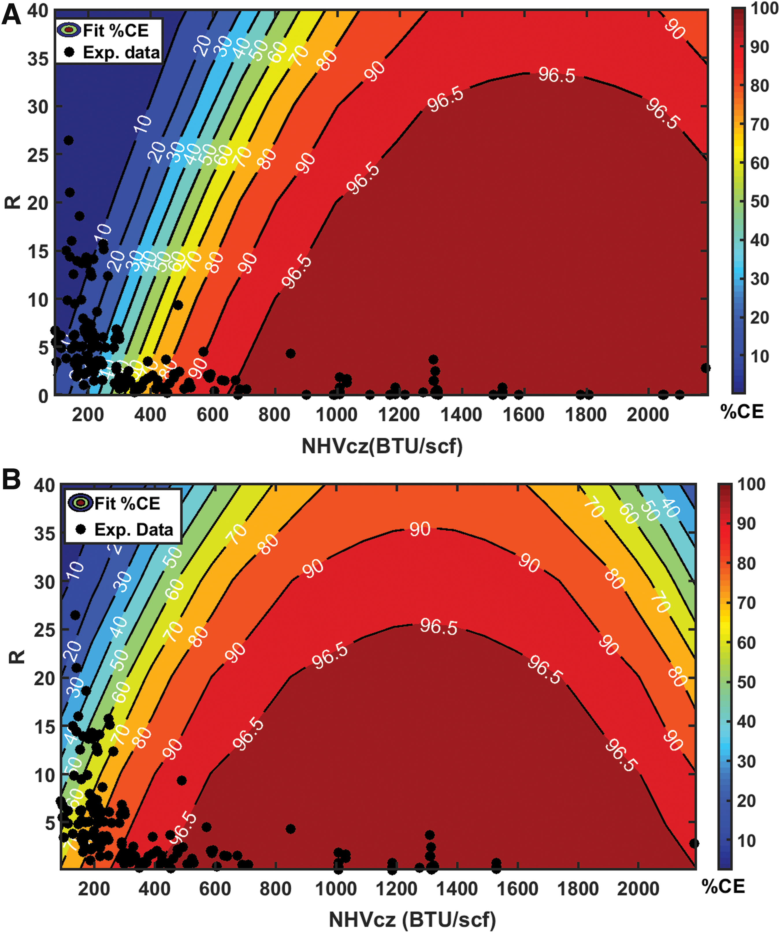
Figure 5A and B shows the 2D contour plot for predicted CE from the Logit (100–CE) model versus NHV_cz, R at two different levels of CHR (0.5 for 100% propene and 0.38 for 100% propane), while S, u, and CN are fixed. Figure 5A and B shows that CE decreases with increase in R for the range of NHV_cz, which substantiates the conclusion that CE increases with increase in exit velocity at a constant crosswind speed for the available data range, and the factors promoting mixing of fuel with steam have a significant effect on combustion. The proposed response surface models are simple quadratic equations applied to predict wide range of experimental data flaring different vent gas mixtures.

FIG. 5.

(A) Two-dimensional contour plot for Logit (100–CE) model showing predicted CE versus NHV_cz, R at CHR = 0.5, S = 0 lb/MMBTU, u = 15 ft/s, and CN = 1.5. (B) Two-dimensional contour plot for Logit (100–CE) model showing predicted CE versus NHV_cz, R at CHR = 0.38, S = 0 lb/MMBTU, u = 15 ft/s, and CN = 1.5.

Response surface models for air-assisted flares

Similarly, response surface models were developed for Logit Opacity and Logit (100–CE) to fit the air-assisted flare test data shown in Table 5. As in the steam-assisted flares, only one of CHR and Pi_vg or Pi_cz is selected for modeling Opacity and CE for air-assisted flares. Table 6 shows the models, N (number of data points), R², and R² (Adj) values, including VE% and MAE% values for the back-calculated Opacity and CE. From the models shown in Table 6, it is clear that A, V, and u (factors influencing mixing), D (laboratory-scale to industrial size flare tips), CHR (for vent gas species), and NHV_dil (dilution parameter) have a significant effect on Logit Opacity, while R (replacing u and V), D, A, CHR, and NHV_dil have a significant effect on Logit (100–CE). The coefficients of assist air in the models imply that increase in assist air decreases the soot emission but increases the emission of unburned VOCs, thereby reducing the CE (Allen and Torres, 2011a, 2011b).

Table 5.

Data Ranges Used in Response Surface Models: Air-Assisted Flares

%Opacity	%CE	NHV_dil (BTU/ft²)	CHR	A (lb/MMBTU)	V (ft/s)	Pi_vg (mol ⁻ ¹)	Pi_cz (mol ⁻ ¹)
0.01–56	80.9–99.9	4–1930	0.275–0.5	0–26238	0.36–72	0–1.8	0–1

Source: Data are from references (McDaniel, 1983; Aerodyne Research Inc., 2010; Allen and Torres, 2011a, 2011b; Fortner et al., 2012; Corbin and Johnson, 2014a, 2014b; Zeng et al., 2016).

NHV_dil, net heating value dilution parameter.

Table 6.

General Quadratic Model Equations for Air-Assisted Flares

Model equations	N	R²	R²_(Adj)	%CE (%Opacity)
Model equations	N	R²	R²_(Adj)	MAE (%)	VE (%)
Logit (100–CE) = −6.53 − 1.9E-09 A² + 2.9E-06 NHV_dil² + 19.3 CHR −19.3 CHR² + 9.4E-05 A − 6.9E-03 NHV_dil ^* D + 0.1767 R − 0.2549 R ^* CHR −0.029 R ^* D	78	0.97	0.96	1.0	90
Logit (100–CE) = −5.392 + 5.46E-04 V² − 1.9E-09A² + 1.4E-05 A ^* V + 1.4E-05 V ^* NHV_dil + 3.6E-04 A − 0.0473 V + 0.1964 MW −6.9E-05 A ^* Pi_vg − 5E-06 A ^* MW −4.4E-03 u ^* Pi_vg + 1.6E-03 NHV_dil ^* Pi_vg − 2.8E-03 MW²	78	0.97	0.97	1.0	90
Logit Opacity = −9.77 − 1.0E-05 A ^* V − 8.3E-06 NHV_dil ^* A +7.96E-04 A ^* CHR +0.0809 u ^* CHR −5E-05 A ^* D + 3.3E-09 A² − 41.04 CHR² − 3.8E-04 A + 39.5 CHR	78	0.96	0.96	1.0	94
Logit Opacity = −1.8865 + 1.73E-06 A ^* u − 2.1E-05 A ^* V + 1.9E-04 NHV_dil − 6.1E-05 A − 0.4966 D − 0.1097 u ^* D + 12.39 Pi_cz − 0.0048 NHV_dil ^* Picz −9.734 Pi_cz² + 0.1890 u − 0.0119 V	78	0.96	0.95	1.1	95

Units and the data range for the models are provided in Table 4; R² and R²_(Adj) represent the correlation between experimental and predicted Logit functions, while MAE% and VE% are between the experimental and the predicted %CE or %Opacity.

Effect of operating parameters on Opacity and CE for air-assisted flares

Opacity predicted by the Logit Opacity model is plotted against NHV_dil and CHR at two levels of A (1,000 and 4,000 lb/millions of BTU [MMBTU]), while other variables were fixed, to analyze the response for change in predictors. Figure 6A and B shows that Opacity increases in the direction toward high CHR and low NHV_dil. Opacity can be higher at a lower NHV_dil due to a lower flame temperature caused by a lower NHV_vg since air assist is fixed at a certain value. Opacity is higher for alkenes (CHR = 0.5) at lower NHV_dil than for alkanes. The contour lines in the 2D plots are intended to show the effect of the operating parameters based on proposed models, while the black dots represent the experimental data.

FIG. 6.

(A) Two-dimensional contour plot for Logit Opacity model showing predicted Opacity versus NHV_dil, CHR at A = 1,000 lb/MMBTU, u = 22 ft/s, and V = 5 ft/s. (B) Two-dimensional contour plot for Logit Opacity model showing predicted Opacity versus NHV_dil, CHR at A = 4,000 lb/MMBTU, u = 22 ft/s, and V = 5 ft/s.

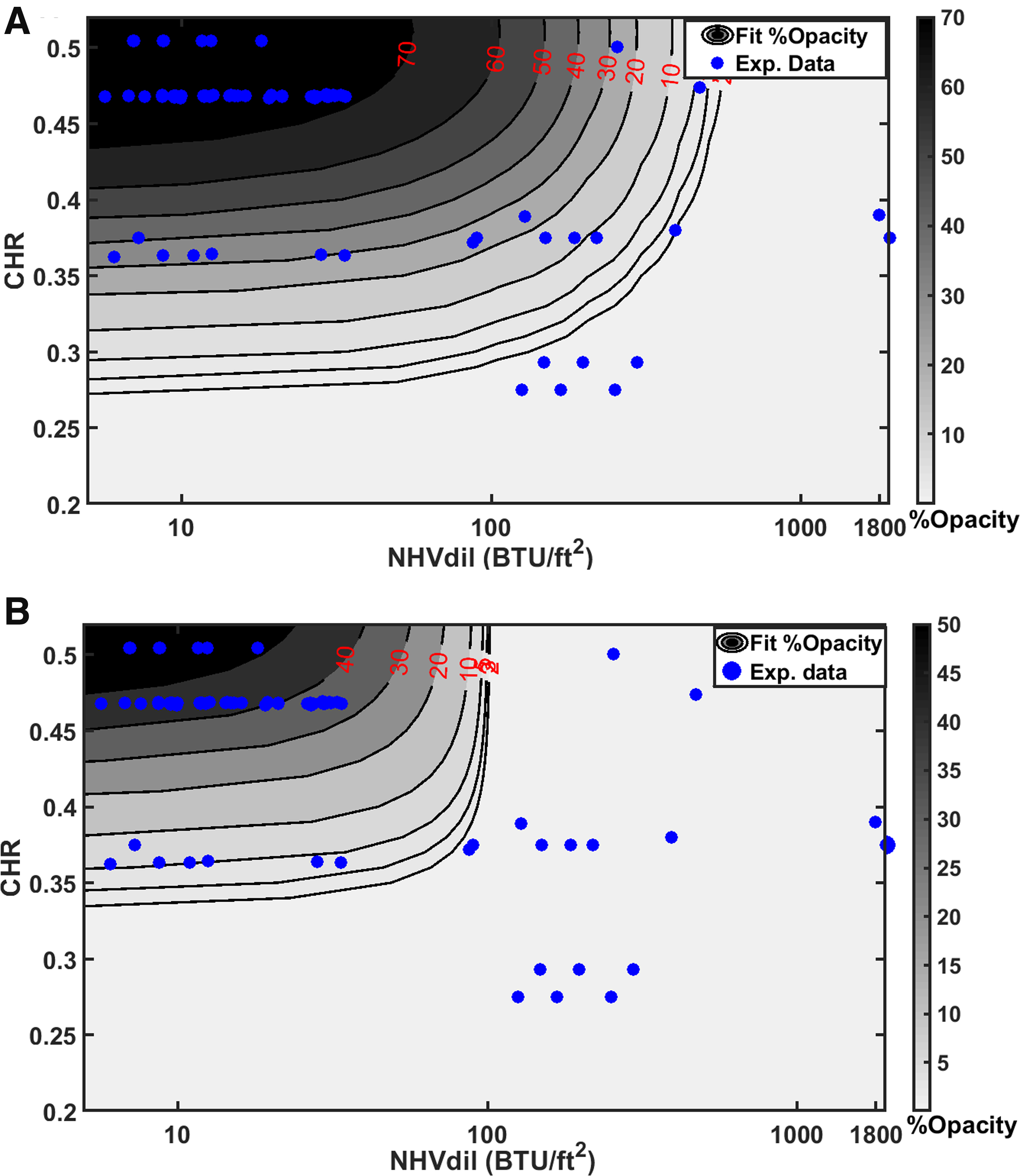
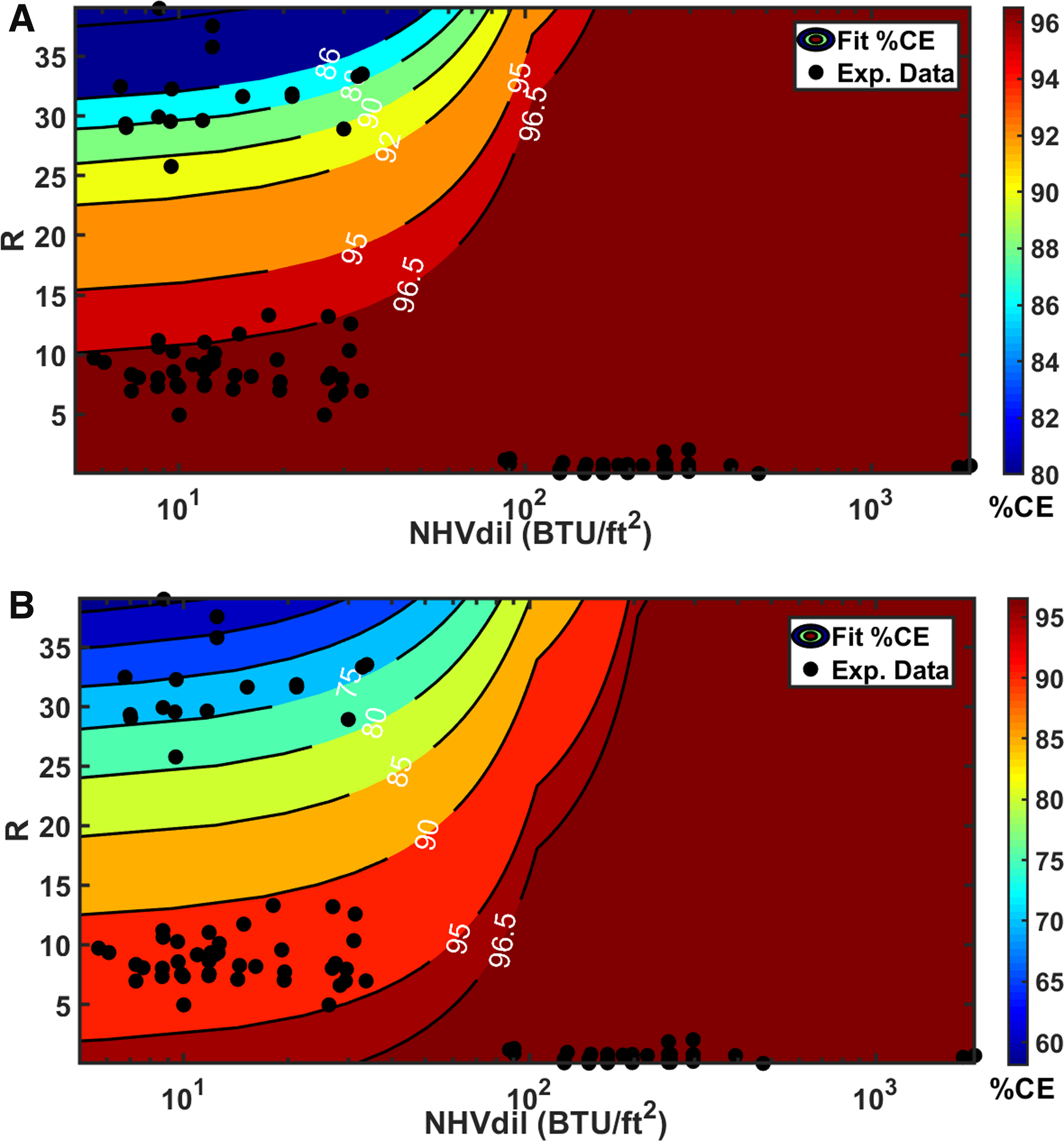
Figure 7A and B shows the 2D contour plot for predicted CE from the Logit (100–CE) model versus NHV_dil, R at two different levels of A, while other variables are fixed. From the Fig. 7A and B, it is observed that CE decreases with an increase in A. Also, increasing R, that is, increasing u or decreasing V, or decreasing NHV_dil lowers CE. Hence, the factors influencing the mixing of fuel with air (R and A) have a significant effect on combustion.

FIG. 7.

(A) Two-dimensional contour plot for Logit (100–CE) model showing predicted CE versus NHV_dil, R at A = 100 lb/MMBTU, CHR = 0.46, and D = 1 ft. (B) Two-dimensional contour plot for Logit (100–CE) model showing predicted CE versus NHV_dil, R at A = 5,000 lb/MMBTU, CHR = 0.46, and D = 1 ft.

Sigmoid models

Sigmoid models for steam-assisted flares

Table 7 shows the univariate and bivariate sigmoid models for CE and corresponding model statistics. The data range for CE, NHV_cz, and V used in these models is shown in Table 2. Twenty-three outliers were removed out of 280 total data points, and the remaining 257 data points were used in univariate models. The univariate sigmoid function is presented to show the derivation of bivariate quadratic equation from a simple sigmoid function. Figure 8 shows a curvature for the univariate model. Since the response variable CE showed a curvature when plotted against NHV_cz, a quadratic form of bivariate sigmoid function was developed further to analyze the effect of important predictors (NHV_cz and V) on the response using response surfaces. Figure 9 shows the 2D contour plot for the response CE versus NHV_cz, V. The proposed quadratic bivariate form of sigmoid function produced reasonable contours for CE versus NHV_cz and V.

FIG. 8.

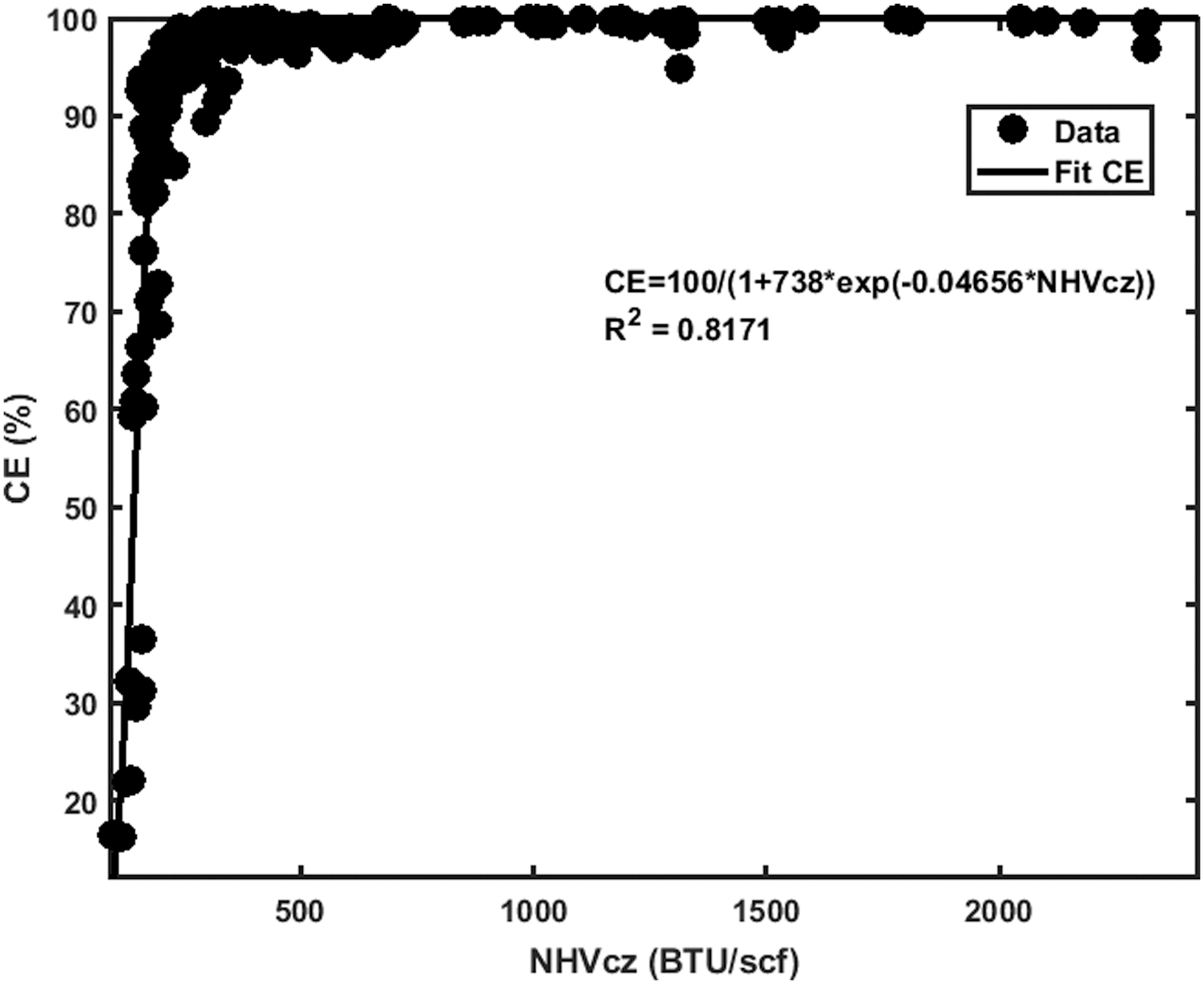
CE versus NHV_cz sigmoid fit for steam-assisted flares.

FIG. 9.

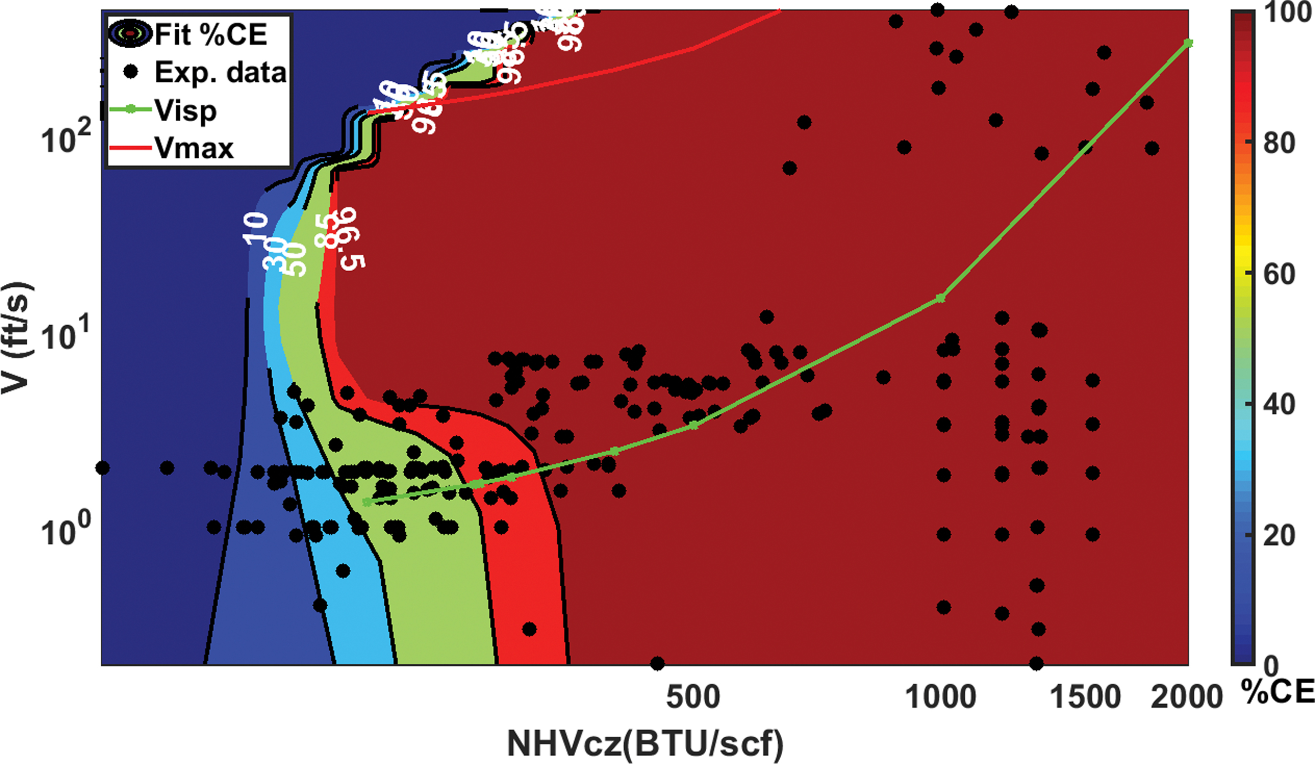
Two-dimensional contour plot of CE versus NHV_cz, V, V_max, and V_ISP for steam-assisted flares.

Table 7.

Univariate and Bivariate Sigmoid Model Equations for Steam-Assisted Flares

Model equation	R²	R²_Adj	RMSE	VE (%)	MAE (%)
CE^a = 100/[1 + 738 ^* exp(−0.04656 ^* NHV_cz)]	0.82	0.81	6.04	81.7	0.78
CE^b = 100/[1 + 1.992 exp (−(0.01697NHV_cz − 4.149V + 0.02NHV_cz ^* V − 0.01V²))]	0.87	0.87	7.48	87.6	2.6

Two hundred fifty-seven data points are used in these models.

Two hundred thirty-three data points are used in these models.

RMSE, root mean square error.

A correlation for maximum exit velocity and NHV_cz is derived from the EPA relation (ECFR, 2015; U.S. EPA, 2015). $\begin{matrix} l o g V_{m a x} & = 1 . 1 E - 03 * N H V_{c z} \\ + 1 . 888 (s t e a m ∕ n o n a s s i s t e d f l a r e s) . \end{matrix}$ (16)

According to Chen and Alphones (2019), the exit velocity at the ISP is expressed as $\begin{matrix} l o g V_{I S P} & = 1 . 3 E - 03 * N H V_{c z} \\ - 1 . 34 E - 01 (s t e a m - a s s i s t e d f l a r e s) . \end{matrix}$ (17)

V_max and V_ISP have been calculated for various values of NHV_cz using these correlations and plotted on the contours of CE in Fig. 9.

V_max and V_ISP for various values of NHV_cz obtained from the above correlations are substituted in the CE model, and the results are shown in Supplementary Table S2 and S3. Figure 9 shows that CE drops at a low velocity (V < 3 ft/s) for NHV_cz < 260 BTU/scf. Furthermore, there is approximately one order of magnitude difference between V_max and V_ISP at the same NHV_cz (Chen and Alphones, 2019). The graph also indicates that CE remains high for NHV_cz > 350 BTU/scf even if the exit velocity exceeds V_max specified by EPA.

Sigmoid models for air-assisted flares

Table 5 shows the data range of V, NHV_dil, and CE used to develop the univariate and bivariate sigmoid models for CE shown in Table 8. Figure 10 shows the sigmoid plot for the univariate model. Since the response variable CE showed a curvature when plotted against NHV_dil, a quadratic form of bivariate sigmoid function was developed further to analyze the effect of important predictors (NHV_dil and V) on the response. Table 8 indicates significant improvement from univariate to bivariate sigmoid function with two parameters (R²_(Adj) changes from 0.83 to 0.91 for bivariate sigmoid with the same number of data points). Figure 11 shows the 2D contour plot of response variable CE on NHV_dil and V plane. The proposed quadratic bivariate form of sigmoid function produced reasonable contours for CE versus NHV_dil and V. To maintain CE ≥96.5%, NHV_dil must be greater than the threshold value ranging from 22 to 500 BTU/ft² over a range of exit velocities as shown in Fig. 11.

FIG. 10.

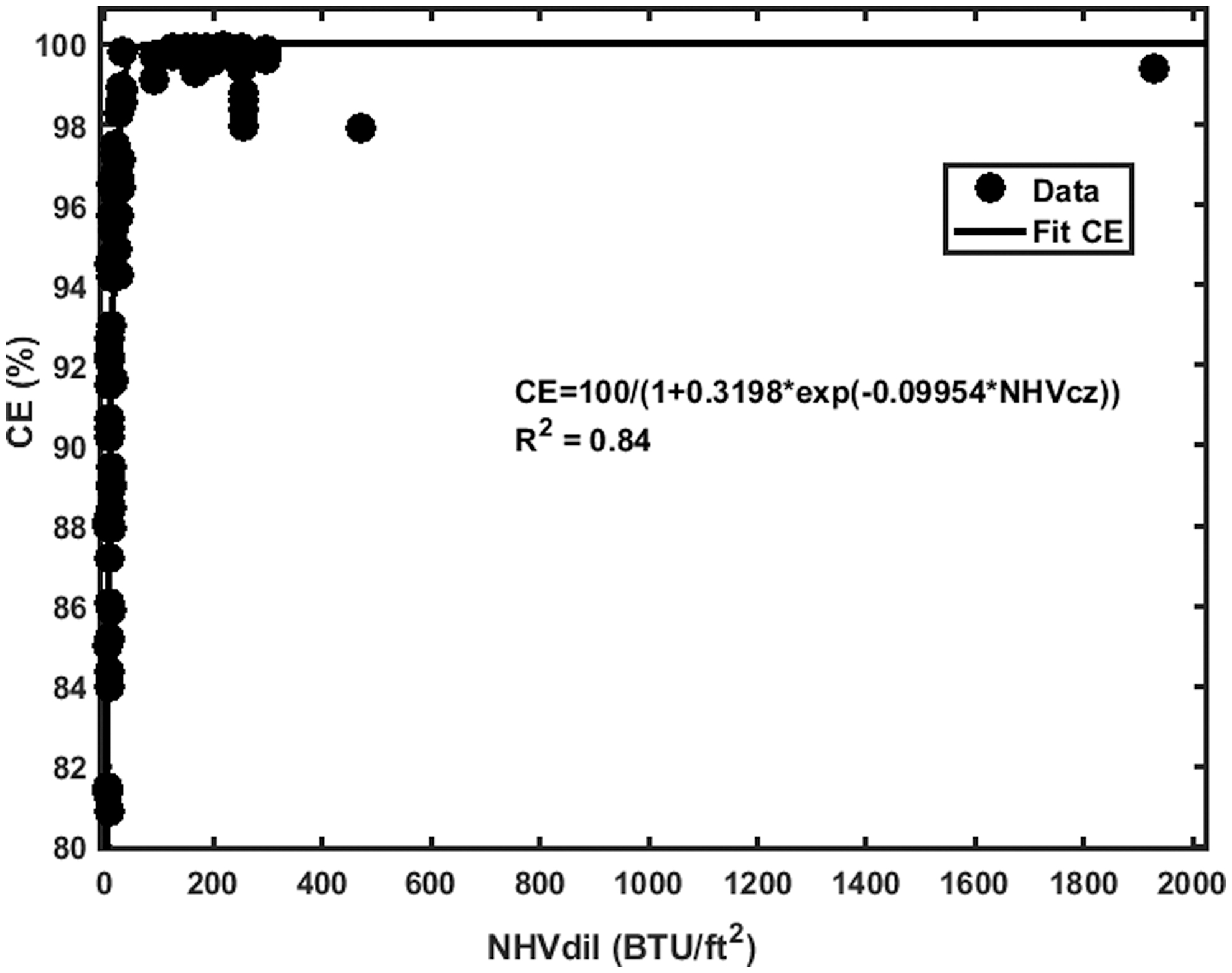
CE versus NHV_dil sigmoid fit for air-assisted flares.

FIG. 11.

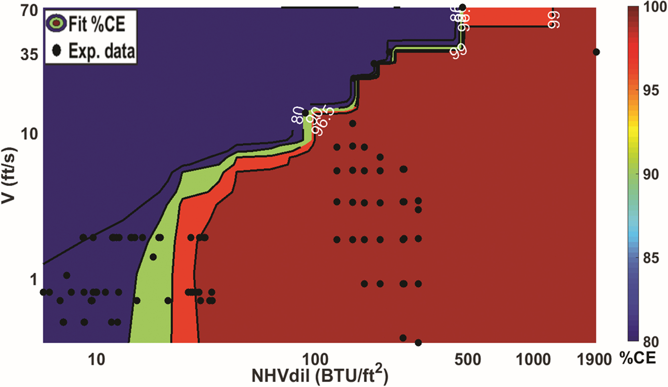
Two-dimensional contour plot of CE versus NHV_dil, V for air-assisted flares.

Table 8.

Univariate and Bivariate Sigmoid Model Equations for Air-Assisted Flares

Model equation	R²	R²_Adj	RMSE	VE (%)	MAE (%)
CE = 100/[1 + 0.3198 ^* exp (−0.09954 ^* NHV_dil)]	0.83	0.83	2.17	83.77	1.48
CE = 100/[1 + 0.4435 ^* exp (−(0.1432 ^* NHV_dil − 0.1234 ^* V + 0.01665 ^* NHV_dil ^* V − 0.12V²))]	0.91	0.91	2.14	85.9	1.32

One hundred two data points are used in these models.

Setpoint determination for steam/air-assisted flares

Based on the ISP characterization for steam- and air-assisted flares, the calculated Opacity range was 1.5–6.6% with an average of 3% Opacity. Ringelmann number 1 corresponds to 20% Opacity, 0.5 corresponds to 10%, and 0.25 corresponds to 5% (Stockham and Betz, 1971; Terry and Ashley, 2013). As the recent EPA regulations require SLF, Opacity <5% is preferred at the discretion of the flare operators.

Setpoint determination for steam-assisted flares

Table 9 shows the comparison of experimental and predicted S, NHV_cz, the required ${Q'}_{f}$ , and CE values for 1984 EPA and 2010 TCEQ test cases at ISP. Test cases S4.1.A, S5.1.A, and S6.1.A represent the average values of the three runs for those tests. The calculated NHV_cz >270 BTU/scf implied that no makeup fuel is required for all steam-assist ISP cases. The predicted steam assist is less than the experimental values for 3% Opacity and NHV_cz ≥ 270 BTU/scf. At a visible emissions rating of 2 (corresponding to 2% Opacity), some tests with high CE produced no visible emissions and the flame was yellowish orange (Cade and Evans, 2010). Hence, Opacity is specified as 2% for SLF conditions based on the VE rating. Table 10 shows the comparison of experimental and predicted values at SLF. Since NHV_cz is a function of S and NHV_vg,req with ${Q'}_{f}$ in its definition, the calculated NHV_cz has multiple solutions satisfying the inequality constraints based on the initial guess for S. However, from an economic standpoint, that is, to minimize the use of makeup fuel and steam, ${Q'}_{f} = 0$ is preferred. Furthermore, minimization of S to increase NHV_cz ≥ 270 BTU/scf is desired. The predicted NHV_cz > 270 BTU/scf at ${Q'}_{f} = 0$ implies that no makeup fuel is required with minimum steam assist. The average setpoints for steam assist (45 lb/MMBTU at SLF and 31 lb/MMBTU at ISP) are less than the experimental average (83 lb/MMBTU) for ISP test cases (Chen and Alphones, 2019). This implies that lower steam assist may be used comparatively to achieve ISP and SLF while complying with the regulations.

Table 9.

Summary of Setpoints for Steam-Assisted Flares at Incipient Smoke Point

Test cases	S (lb/MMBTU)		NHV_cz (BTU/scf)		VG/Fuel (scf/hr)		%Opacity		%CE
Test cases	Exp	Pred	Exp	Pred	Q_vg	$Q'_{f}$	Exp	Pred	Exp	Pred
S.1.5.1	94	64	405	545	21440	0	0.2	3	99.9	97.2
S.4.1.A	101	18	202	306	30260	0	0.1	3	95.8	99.6
S.5.1.A	111	56	251	345	11580	0	4.3	3	95.5	98.8
S.6.1.A	84	56	293	354	29660	0	3	3	99.1	99.4
S.8.3.1	84	19	219	308	18318	0	7.2	3	95.9	96.5
105	2.4	2.3	1531	2104	13913	0	2.5	3	99.7	99.7
94	3.0	2.7	2045	2065	14020	0	2.2	3	99.8	99.7

Exp, experimental; MMBTU, millions of BTU; Pred, predicted.

Table 10.

Summary of Setpoints for Steam-Assisted Flares at Smokeless Flaring

Test cases	S (lb/MMBTU)		NHV_cz (BTU/scf)		VG/fuel (scf/hr)		%Opacity		%CE
Test cases	Exp	Pred	Exp	Pred	Q_vg	$Q'_{f}$	Exp	Pred	Exp	Pred
S.1.5.1	94	75	405	481	21440	0	0.2	2	99.9	95.8
S.4.1.A	101	40	202	270	30260	0	0.1	2	95.8	99.3
S.5.1.A	111	79	251	295	11580	0	4.3	2	95.5	98.2
S.6.1.A	84	79	293	288	29660	0	3	2	99.1	98.8
S.8.3.1	84	39	219	271	18318	0	7.2	2	95.9	95.9
105	2.4	2.5	1531	2091	13913	0	2.5	2	99.7	99.7
94	3.0	3.0	2045	2049	14020	0	2.2	2	99.8	99.7

Comparison of setpoints at ISP and SLF for steam-assisted flares

Figure 12A–C shows the comparison of predicted S, NHV_cz, and CE (at ISP and SLF) with experimental values for steam-assisted flares. The average of predicted setpoints for steam assist (31 lb/MMBTU at the ISP and 45 lb/MMBTU at SLF) lies below the experimental steam assist, 57 lb/MMBTU (geometric mean, x₅₀) for ISP test cases. Since no makeup fuel is required at ISP and SLF, the NHV_vg,req remains the same. The discrepancy between the predicted ISP steam/makeup fuel and experimental data can be attributed to (1) the simplicity of the quadratic form even with the transforms; (2) the observed ISP's uncertainties caused by human observation errors (as seen by the wide variations in characterized Opacity, CE, heating value, etc. at the ISP); and (3) the ISP or SLF can be achieved in multiple states experimentally by simultaneously increasing NHV_vg,req (NHV_vg and makeup fuel) and the diluent (steam) for better mixing. Due to minimization of steam assist at ISP and SLF, the predicted CE is maximized (98.6% at ISP and 98% SLF) compared with 97.6% for the experimental ISP cases.

FIG. 12.

(A) Comparison of setpoints of steam assist in compliance with EPA regulations for steam-assisted flares. (B) Comparison of setpoints of NHV_cz in compliance with EPA regulations for steam-assisted flares. (C) Comparison of setpoints of CE (%) in compliance with EPA regulations for steam-assisted flares. EPA, Environmental Protection Agency.

Setpoint determination for air-assisted flares

Table 11 shows the comparison of experimental and predicted values of A, NHV_dil, CE, and the required ${Q'}_{f}$ when calculated NHV_dil < 22 BTU/ft² for the 2010 TCEQ test cases at ISP. Letter “A” at the end (e.g., A2.1.A, A3.1.A, etc.) denotes the average values of the three experimental runs. Since the experimental Opacity values were >3% for cases A1.1.1, A2.1.A, and A6.1.A, the solution converged to 4% with ${Q'}_{f} = 0$ . Hence, ${Q'}_{f}$ is required to maintain NHV_dil at 22 BTU/ft² for 3% Opacity. For other cases with the experimental Opacity ≤3%, air assist decreases to increase Opacity to 3%. Hence, those cases require assist air less than the experimental value. For example, in case A7.1.A the assist air decreases to increase the Opacity to 3%, thereby increasing NHV_dil from 31 to 322 BTU/ft².

Table 11.

Summary of Setpoints for Air-Assisted Flares at the Incipient Smoke Point

Test cases	A (lb/MMBTU)		NHV_dil (BTU/ft²)		VG/Fuel (scf/hr)		%Opacity		%CE
Test cases	Exp	Pred	Exp	Pred	Q_vg	$Q'_{f}$	Exp	Pred	Exp	Pred
A1.1.1	8247	7166	18.2	22	8602	1004	4.1	3	96.7	97.2
A2.1.A	12000	7400	12.5	22	3295	635	3.9	3	96.1	98.3
A3.1.A	4952	4882	29.2	30	11768	0	3.1	3	98.1	98.1
A4.1.A	7601	4253	19.4	34	11657	0	2.1	3	97	98.5
A5.1.A	5251	2208	27.5	62	4613	0	1.8	3	95.9	99.6
A6.1.A	4553	7060	32.2	22	4413	140	6.2	3	98.8	96.6
A7.1.A	5104	261	31	322	4758	0	0.04	3	99.8	99.9

Table 12 shows the comparison of experimental and predicted values at SLF. Since NHV_dil is a function of A and NHV_vg,req with ${Q'}_{f}$ in its equation, the calculated NHV_dil has multiple solutions based on the initial guess for A. However, from an economic standpoint, that is, to minimize the use of makeup fuel, $Q'_{f} = 0$ is preferred. Furthermore, minimization of A to increase NHV_dil ≥ 22 BTU/ft² is desired. Lowest values of assist air and makeup fuel were chosen as the solution. Similar to the ISP conditions, for cases A1.1.1, A2.1.A, and A6.1.A, ${Q'}_{f}$ is required to maintain NHV_dil at 22 BTU/ft², whereas for other cases predicted assist air increases or decreases compared with experimental value to maintain Opacity at 2% and NHV_dil ≥ 22 BTU/ft². The average of predicted A and ${Q'}_{f}$ at ISP and SLF are 4,747 lb/MMBTU and 254 scf/h and 5,737 lb/MMBTU and 659 scf/h, respectively.

Table 12.

Summary of Setpoints for Air-Assisted Flares at Smokeless Flaring

Test cases	A (lb/MMBTU)		NHV_dil (BTU/ft²)		VG/Fuel (scf/hr)		%Opacity		%CE
Test cases	Exp	Pred	Exp	Pred	Q_vg	$Q'_{f}$	Exp	Pred	Exp	Pred
A1.1.1	8247	7931	18.2	22	8602	3100	4.1	2	96.7	96.9
A2.1.A	12000	7841	12.5	22	3295	1098	3.9	2	96.1	98.1
A3.1.A	4952	6644	29.2	22	11768	0	3.1	2	98.1	96.8
A4.1.A	7601	5973	19.4	25	11657	0	2.1	2	97	97.3
A5.1.A	5251	3575	27.5	40	4613	0	1.8	2	95.9	98.9
A6.1.A	4553	7768	32.2	22	4413	415	6.2	2	98.8	96.2
A7.1.A	5104	430	31	237	4758	0	0.04	2	99.8	99.9

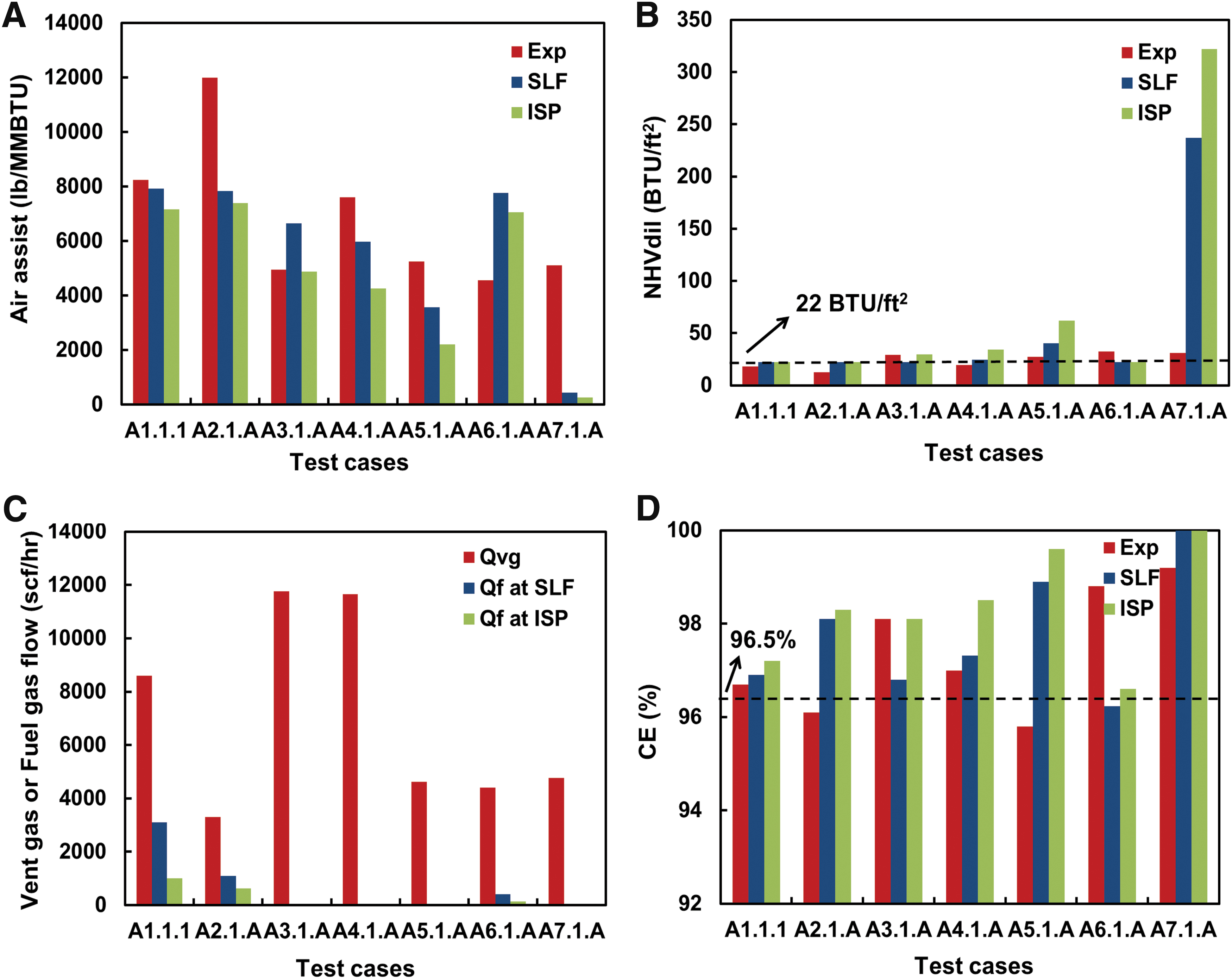
Comparison of setpoints at ISP and SLF for air-assisted flares

Figure 13A–D shows the comparison of predicted and experimental values of A, NHV_dil, ${Q'}_{f}$ , and CE (at ISP and SLF) for air-assisted flares. The average predicted setpoints of assist air (4,747 lb/MMBTU at ISP and 5,737 lb/MMBTU at SLF) lie below the experimental value (6,170 lb/MMBTU, (x₅₀)) for ISP test cases. Since minimum makeup fuel is required at ISP and SLF, NHV_vg,req is calculated. The average of predicted NHV_vg,req (879 BTU/scf at ISP and 842 BTU/scf at SLF) is lower than the experimental average (920 BTU/scf). The discrepancy between the predicted assist air/makeup fuel and the experimental data can be attributed to (1) the simplicity of the quadratic form even with the transforms; (2) the observed ISP's uncertainties caused by human observation errors (as seen by the wide variations in characterized Opacity, CE, heating value, etc. at the ISP); and (3) the ISP or SLF can be achieved in multiple states experimentally by simultaneously increasing NHV_vg,req (NHV_vg and makeup fuel) and the diluent (air) to influence better mixing. Therefore, ISP or SLF is achieved by simultaneously adding makeup fuel and assist air or by reducing air assist alone. Due to the minimization of air at ISP and SLF, predicted CE increases (98.3% at ISP and 97.8% SLF) compared with 97.1% for the experimental ISP test cases (Chen and Alphones, 2019).

FIG. 13.

(A) Comparison of setpoints of assist air in compliance with EPA regulations for air-assisted flares. (B) Comparison of setpoints of NHV_dil in compliance with EPA regulations for air-assisted flares. (C) Comparison of setpoints of ${Q'}_{f}$ in compliance with EPA regulations for air-assisted flares. (D) Comparison of setpoints of CE (%) in compliance with EPA regulations for air-assisted flares.

Conclusions

General quadratic response surface models for transformed Opacity (Log Abs for steam and Logit Opacity for air) and CE were developed for both steam- and air-assisted flares based on the experimental flare study data collected from 1983 through 2016 for which soot and CE values were available. Reported CE in the literature was corrected for soot emissions. The major conclusions of this study are as follows: 1.

The goodness-of-fit (R²) values for CE and Opacity models with the operation parameters were 0.93 and 0.91 for steam-assisted flares and 0.98 and 0.95 for air-assisted flares, respectively.

Best subsets regression method was used to determine the best set of variables for the Opacity and CE models. The parameters that influence mixing with ambient air for the flares with tips ranging from laboratory scale to industrial scale burning vent gas species with natural gas mixtures (C₁) to olefin mixtures (C₂ and C₃) and the NHV_dil were found to have a significant effect on Opacity and CE models developed for air-assisted flares. The parameters that influence mixing with ambient air for the flares burning vent gas species with natural gas mixtures (C₁) to olefin mixtures (C₂ and C₃) and the NHV_cz were found to have a significant effect on Opacity and CE models developed for steam-assisted flares.

Bivariate sigmoid models for steam- and air-assisted flares showed a good agreement with the experimental data with the goodness of fit >0.9. Two-dimensional contours developed to analyze the effect of major parameters on the response variable CE showed that the NHV_cz >270 BTU/scf (for steam-assisted flares) and NHV_dil > 22 BTU/ft² (for air-assisted flares) are required to achieve CE >96.5%.

The discrepancy between the predicted steam assist/air assist/makeup fuel and experimental data may arise from (1) the simplicity of the quadratic form of the response surface models; and (2) the uncertainties caused by human observation errors of Opacity as seen from the wide variations in characterized Opacity values at the ISP; and (3) the existence of multiple states experimentally with simultaneous increase of vent gas heating values and steam/air assists.

Setpoints would help flare operators to establish ISP or SLF conditions either by adding makeup fuel to the vent gas with low heating value along with the assist or by minimizing the air or steam assist alone. From an economic standpoint, ${Q'}_{f} = 0$ with low air or steam assist is preferred.

Footnotes

Acknowledgments

We specially thank Ed Fortner and Scott Herndon of Aerodyne Research Inc., Scott Evans from Clean Air Engineering, Dr. Darcy Corbin and Dr. Matthew Johnson from Carleton University, and Dr. Yousheng Zeng from Providence Photonics for providing the flare test data.

Author Disclosure Statement

No competing financial interests exist.

Disclaimer Language

The content, findings, opinions, and conclusions are the work of the author(s) and do not necessarily represent findings, opinions, or conclusions of the TCEQ.

Funding Information

The authors gratefully acknowledge the financial support from TCEQ Grant for Activities Program (Project # 582-10-94307-FY14-06), TCEQ Supplemental Environmental Program (SEP Agreement No. 2009-009), and the Texas Air Research Center (TARC Grant #079LUB0096A).

Supplementary Material

Nomenclature

Subscripts:

References

Aerodyne Research, Inc. (2010). APPENDIX Aerodyne Research Mobile Laboratory Particulate Measurements TCEQ 2010 Flare Study. Prepared for TCEQ: Austin, TX.

Allen

D.T.

, and Torres

V.M.

(2011a). TCEQ 2010 Flare Study Final Report; The University of Texas at Austin, The Center for Energy and Environmental Resources; TCEQ PGA No. 582-8-86245-FY09-04 and Task Order No. UTA10-000924-LOAT-RP9; Austin, TX.

Allen

D.T.

, and Torres

V.M.

(2011b). 2010 Flare study final appendices. Available at: https://www.tceq.texas.gov/assets/public/implementation/air/rules/Flare/2010flarestudy/2010-flare-study-final-appendices.pdf (accessed March 8, 2014).

Anenberg

S.C.

, Schwartz

, Shindell

, Amann

, Faluvegi

, Klimont

, Jansenns-Maenhout

, Pozzoli

, van Dingenen

, Vignati

, Emberson

, Muller

N.Z.

, West

J.J.

, Williams

, Demkine

, Hicks

W.K.

, Kuylenstrina

, Raes

, and Ramanathan

(2012). Global air quality and health co-benefits of mitigating near-term climate change through methane and black carbon emission controls. Environ. Health Perspect. 120, 831.

Bates

, and Watts

(1988). Nonlinear Regression Analysis and Its Applications. New York: Wiley & Sons.

Bates

D.M.

, and Chambers

J.M.

(1992). Nonlinear models. In J.M. Chambers, and T.J. Hastie, Eds., Statistical Models in S. California: Wadsworth, p. 421.

Bond

T.C.

, Doherty

S.J.

, Fahey

D.W.

, Forster

P.M.

, Berntsen

, Deangelo

B.J.

, Flanner

M.G.

, Ghan

, Kärcher

, Koch

, Kinne

, Kondo

, Quinn

P.K.

, Sarofim

M.C.

, Schultz

M.G.

, Schulz

, Venkataraman

, Zhang

, Bellouin

, Guttikunda

S.K.

, Hopke

P.K.

, Jacobson

M.Z.

, Kaiser

J.W.

, Klimont

, Lohmann

, Schwarz

J.P.

, Shindell

, Storelvmo

, Warren

S.G.

, and Zender

C.S.

(2013). Bounding the role of black carbon in the climate system: A scientific assessment. J. Geophys. Res. Atmos. 118, 5380.

Cade

, and Evans

(2010). Performance Test of a Steam–Assisted Elevated Flare with Passive FTIR. Marathon Petroleum Company, Texas City Main Flare; Project No: 10810; Final Report prepared by Clean Air Engineering, Inc.: Texas City, TX.

Castiñeira

, and Edgar

T.F.

(2006). CFD for simulation of steam-assisted and air-assisted flare combustion systems. Energy Fuels. 20, 1044.

10.

Chen

D.H.

, and Alphones

(2019). Characterization of the incipient smoke point for steam-/air-assisted and non-assisted flares. J. Air Waste Manag. Assoc. 69, 119.

11.

Corbin

D.J.

, and Johnson

M.R.

(2014a). Interim Report: Summary of Flare Efficiency and Soot Emission Rate Measurement Results to Date at Carleton University Energy & Emissions Research Lab. Introduction & Test Overview; No. 582, 1.

12.

Corbin

D.J.

, and Johnson

M.R.

(2014b). Detailed expressions and methodologies for measuring flare combustion efficiency, species emission rates, and associated uncertainties. Ind. Eng. Chem. Res. 53, 19359.

13.

CyboSoft. Model-Free Adaptive Control of Flare Heating Value Process. Available at: http://www.cybosoft.com/pdf/ATS_50_MFA-Flare-Heating-Value-Process-Control.pdf (accessed October 20, 2016).

14.

Damodara

, Chen

D.H.

, Lou

H.H.

, Rasel

K.M.A.

, Richmond

, Wang

, and Li

(2017). Reduced combustion mechanism for C1–C4 hydrocarbons and its application in computational fluid dynamics flare modeling. J. Air Waste Manag. Assoc. 67, 599.

15.

ECFR. (2015). General Control Device and Work Practice Requirements. Available at: http://www.ecfr.gov/cgi-bin/text-idx?SID = a70febff19f3282c2e40d939bf61f72c&mc = true&node = se40.7.60_118&rgn = div8 (accessed December 20, 2015).

16.

ENVIRON International Corporation. (2008). Cost Analysis of HRVOC Controls on Polymer Plants and Flares, Project 2008–104, Work Order 582-07-84005-FY-08-12; Prepared for Texas Commission on Environmental Quality: Austin, TX.

17.

ENVIRON International Corporation. (2009). Cost Analysis of Highly Reactive Volatile Organic Compound Controls on Refineries and Chemical Plants-Project 2009–52; Control of HRVOC Emissions in Flares at Low Flow Conditions-Project 2009–53; Prepared for Texas Commission on Environmental Quality: Austin, TX. Available at: https://www.tceq.texas.gov/assets/public/implementation/air/rules/contracts/2009-hrvoc-cost-analysis-final.pdf (accessed February 20, 2016).

18.

Fortner

E.C.

, Brooks

W.A.

, Onasch

T.B.

, Canagaratna

M.R.

, Massoli

, Jayne

J.T.

, Franklin

J.P.

, Knighton

W.B.

, Wormhoudt

, Worsnop

D.R.

, Kolb

C.E.

, and Herndon

(2012). Particulate emissions measured during the TCEQ comprehensive flare emission study. Ind. Eng. Chem. Res. 51, 12586.

19.

Fox

(2008). Applied Regression Analysis and Generalized Linear Models. California: Sage.

20.

Fry

C.R.

, and Coburn

(2012). Peer review of “Parameters for Properly Designed and Operated Flares”, Memorandum. Prepared for A. Bouchard and B. Shine, EPA/OAQPS. Available at: https://www.epa.gov/sites/production/files/2016-06/documents/2012flarepeerreviewmemo.pdf (accessed August 21, 2016).

21.

Gallant

A.R.

(1975). Nonlinear regression. Am Stat. 29, 73.

22.

Gallik

Transmittance and Absorbance. Available at: http://cellbiologyolm.stevegallik.org/node/7 (accessed March 29, 2017).

23.

Ghoreishian

S.M.

, Badii

, Norouzi

, and Malek

(2016). Effect of cold plasma pre-treatment on photocatalytic activity of 3D fabric loaded with nano-photocatalysts: Response surface methodology. Appl. Surf. Sci. 365, 252.

24.

Homayoonfal

, Khodaiyan

, and Mousavi

(2015). Modeling and optimizing of physicochemical features of walnut-oil beverage emulsions by the implementation of response surface methodology: Effect of preparation conditions on emulsion stability. Food Chem. 174, 649.

25.

Jacobson

, Bond

T.C.

, Lam

N.L.

, and Hultman

(2013). Black Carbon and Kerosene Lighting: An opportunity for rapid action on climate change and clean energy for development. Washington, DC: The Brookings Institution. Available at: https://www.brookings.edu/wp-content/uploads/2016/06/04_climate_change_clean_energy_development_hultman.pdf (accessed October 10, 2019).

26.

Jäger

, Henning

, Schlögl

, and Spillecke

(1999). Spectral properties of carbon black. J. Non Cryst. Solids, 258, 161.

27.

Korppoo

(2018). Russian associated petroleum gas flaring limits: Interplay of formal and informal institutions. Energy Policy. 116, 232.

28.

Levitsky

(2011). Climate change series black carbon and climate change—Considerations for international development agencies. Environ. Dep. Pap. 112, 52.

29.

(2017). Assessing the accuracy of predictive models for numerical data: Not r nor r², why not? Then what?. PLoS One, 12, e0183250.

30.

, Han

, Sun

, Lu

, and Ding

(2015). Optimization of acidified oil esterification catalyzed by sulfonated cation exchange resin using response surface methodology. Energy Convers. Manag. 98, 46.

31.

MathWorks, Inc. (2015). MATLAB and Curvefitting Toolbox R2015b. Natick, Massachusetts.

32.

McDaniel

(1983). Flare Efficiency Study; EPA-600/2-83-052; EPA Contract 68-02-3541-6; Prepared for U.S. Environmental Protection Agency, Office of Research and Development, Washington, DC; Industrial Processes Branch, Industrial Environmental Research Laboratory: Research Triangle Park, NC.

33.

Minitab. (2018). Customize the probability plot. Available at: http://support.minitab.com/en-us/minitab-express/1/help-and-how-to/graphs/probability-plot/create-the-graph/customize-the-probability-plot/ (accessed December 17, 2018).

34.

Pan

, Choi

, Roy

, Li

, Jeon

, and Souri

A.H.

(2015). Modeling the uncertainty of several VOC and its impact on simulated VOC and ozone in Houston, Texas. Atmos. Environ. 120, 404.

35.

Pohl

; Payne

, and Lee

(1984). Evaluation of the efficiency of industrial flares: Test Results; EPA-600/2-84-095; Prepared for U.S. EPA Office of Research and Development; Energy and Environmental Research Corporation: California.

36.

Ratkowsky

D.A.

(1990). Handbook of Nonlinear Regression Models. New York: Marcel Dekker.

37.

Roesler

, Evans

, Schmid

, and Wright

(2010). Performance Test of a Steam—Assisted Elevated Flare with Passive FTIR—Detroit Table of Contents. Marathon Petroleum Company, Detroit; Project No: 10971; Final Report prepared by Clean Air Engineering, Inc.: Detroit, MI.

38.

Schwartz

J.P.

, Holloway

J.S.

, Katich

J.M.

, Mckeen

, Kort

E.A.

, Smith

M.L.

, Ryerson

T.B.

, Sweeney

, and Peischl

(2015). Black carbon emissions from the Bakken Oil and Gas development region. Environ. Sci. Technol. Lett. 2, 281.

39.

Schwartz

, White

, and Bussman

(2001). The John Zink Combustion Handbook. (C.E.J. Baukal and R. Schwartz, Eds.). New York: CRC Press.

40.

Singh

K.D.

, Dabade

, Vaid

, Gangadharan

, Chen

, Lou

H.H.

, Li

, and Martin

C.B.

(2012). Computational fluid dynamics modeling of industrial flares operated in stand-by mode. Ind. Eng. Chem. Res. 51, 12611.

41.

Singh

K.D.

, Gangadharan

, Chen

D.H.

, Lou

H.H.

, Li

, and Richmond

P.C.

(2014a). CFD modeling of laboratory flames and industrial flares. J. Air Waste Manag. Assoc. 64, 1328.

42.

Singh

K.D.

, Gangadharan

, Dabade

, Shinde

, Chen

, Lou

H.H.

, Richmond

P.C

, and Li

(2014b). Parametric study of ethylene flare operations using numerical simulation. Eng. Appl. Comp. Fluid Mech. 8, 211.

43.

Smith

(2012). Modeling Flare Destruction and Removal Efficiency, Southeast Texas Photochemical Modeling Technical Committee, Houston, TX.

44.

Srinivasarao

, and Krishna

K.M.

(2015). A brief overview of soot formation theory and soot reduction methods in steam-assisted flares. Int. J. Environ. Sci. Toxicol. Res. 3, 49.

45.

Srinivasarao

, and Krishna

K.M.

(2017). Feed forward control method to reduce soot from steam assisted flares. J. Environ. Res. Dev. 11, 558.

46.

Stockham

, and Betz

(1971). Study of visible exhaust smoke from aircraft jet engines. FAA-RD-71-22. IIT Research Institute. Chicago, IL. Prepared for Department of Transportation, Federal Aviation Administration, Washington D.C.

47.

Stohl

, Klimont

, Eckhardt

, Kupiainen

, Shevchenko

V.P.

, Kopeikin

V.M.

, and Novigatsky

A.N.

(2013). Black carbon in the Arctic: The underestimated role of gas flaring and residential combustion emissions. Atmos. Chem. Phys. 13, 8833.

48.

Terry

, and Ashley

(2013). Visible Emissions Observer Training Manual. Garner, NC: Eastern Technical Associates, Inc.

49.

U.S. EPA. (2009). Stationary point and area sources. AP 42, Compilation of Air Pollutant Emissions Factors, 1, 13.5-1–13.5-5.

50.

U.S. EPA. (2012). Office of Civil Enforcement. Enforcement Alert, EPA 325-F-012-002. Available at: https://www.epa.gov/sites/production/files/documents/flaringviolations.pdf (accessed March 31, 2018).

51.

U.S. EPA. (2015). Petroleum refinery sector risk and technology review and new source performance standards. Vol. 80, No. 230. Available at: https://www.govinfo.gov/content/pkg/FR-2015-12-01/pdf/2015-26486.pdf (accessed October 10, 2017).

52.

U.S. EPA. (2018a). AP 42, Fifth Ed. Volume I. Chapter 13: Miscellaneous Sources. Available at: https://www3.epa.gov/ttn/chief/ap42/ch13/final/C13S05_02-05-18.pdf (accessed October 10, 2019).

53.

U.S. EPA. (2018b). National emission standards for hazardous air pollutants and new source performance standards: Petroleum refinery sector amendments. Vol. 83, No. 227. 60696-60728. Available at: https://www.govinfo.gov/content/pkg/FR-2018-11-26/pdf/2018-25080.pdf (accessed January 10, 2019).

54.

World Bank. (2018). Gas Flaring Data 2013–17. Available at: www.worldbank.org/en/programs/gasflaringreduction#7 (accessed May 23, 2018).

55.

Zeng

, Morris

, and Dombrowski

(2016). Validation of a new method for measuring and continuously monitoring the efficiency of industrial flares. J. Air Waste Manag. Assoc. 66, 76.

Supplementary Material

Please find the following supplemental material available below.

For Open Access articles published under a Creative Commons License, all supplemental material carries the same license as the article it is associated with.

For non-Open Access articles published, all supplemental material carries a non-exclusive license, and permission requests for re-use of supplemental material or any part of supplemental material shall be sent directly to the copyright owner as specified in the copyright notice associated with the article.

0.00 MB

0.13 MB