Prediction of PM 2.5 Concentrations Using Principal Component Analysis and Artificial Neural Network Techniques: A Case Study: Urmia,Iran

Abstract

Forecasting PM_2.5 concentration in ambient air quality is of great concern to urban management administrative due to its harmful health consequences and interference with the safe and comfortable use of the environment. In this study, the prediction of PM_2.5 concentration using three artificial neural network models, including multi-layer perceptron (MLP), radial basis function (RBF), and generalized regression neural network was investigated. The effect of principal component analysis (PCA) technique on improving the results was studied as well. Urmia City, Iran, was selected as the case study. Air pollution parameters, that is, NO₂, CO, PM₁₀, and PM_2.5 were obtained from Urmia air quality monitoring station No. 3 and meteorological data, including temperature, relative humidity, and wind speed, were collected from the Urmia airport synoptic station. Three scenarios of input data were proposed to address the effect of time lag. According to the results, the highest correlation coefficient (R²) and the minimum values of mean squared error and mean absolute error parameters were obtained from RBF network with input data scenario No. 2 (including the data of 1 and 2 days before the forecasting). PCA application not only reduced the number of input data in MLP network but also increased the correlation coefficient between real data and the predicted one by 3.8%. Due to the fact that NO₂, as the major source of nitrate aerosols, has low retention time in the atmosphere (1–2 days), and considering the significant relationship between PM_2.5 and NO₂ concentrations in Urmia city, it can be concluded that the data of 3 days before the forecasting day might not contribute meaningfully in PM_2.5 prediction.

Introduction

Nowadays, air pollution as an emerging phenomenon, has become one of the most important environmental issues of many cities throughout the world. According to the World Health Organization (WHO, 2018), 91% of the world's population lives in places where air quality levels exceed WHO limits. The U.S. Environmental Protection Agency (U.S. EPA) has determined six pollutants, including particulate matter (PM_2.5 and PM₁₀), NO₂, SO₂, CO, O₃, and Lead, as “criteria air pollutants” among them; particulate matter has gained the most researchers' attention due to its adverse effects on human health. According to WHO, airborne PM is a complex mixture of solid and liquid particles suspended in the air that varies continuously in size and chemical composition in space and time.

The major components of PM are sulfates, nitrates, ammonia, sodium chloride, black carbon, mineral dust, and water (WHO, 2018). Particulate matter is classified based on different criteria. Aerodynamic diameter is an important characteristic to explain the ability of particles to transport in the atmosphere and their penetration in the respiratory tract. The USEPA classifies particulate matter based on aerodynamic diameter into two major groups: particles with an aerodynamic diameter <10 μm (PM₁₀) and units with an aerodynamic diameter <2.5 μm (PM_2.5).

Studies on particulate matter show that PM_2.5 is more likely to affect human health than PM₁₀ (Spurny, 1998; Klemm et al., 2000; Schwartz and Neas, 2000). An important characteristic of PM_2.5 is their lifetimes (from 1 day to 1 week) and their ability to be transported from hundreds to thousands of kilometers (Kim et al., 2015). Major sources of PM_2.5 emissions in urban environments include fossil fuel combustion gases in motor vehicles, heating systems of residential buildings, power plants, and industries (Martins and da Graça, 2018). Particles deposition in the lungs and their high potential for adsorption of toxic air pollutants such as organic compounds and heavy metals may cause cardiovascular and respiratory diseases and lung cancer (Brook et al., 2002; Pope et al., 2002). WHO air quality control guidelines estimate that if annual average of PM_2.5 concentrations is reduced from level of 35 μg/m³ to 10 (10 equals to the WHO guideline level), in many developed cities, air pollution-related deaths will be reduced around 15% (WHO, 2018). In a study, Jung et al. (2015) showed that a 4.34 μg/m³ increase in PM_2.5 concentration might lead to a 138% increase in the risk of Alzheimer's disease. Therefore, developing a model to forecast the concentration of this pollutant for the next days is necessary to manage the air pollution in metropolises.

Several methods have been developed recently to predict the concentration of air pollutants, which could be divided into two main groups: deterministic and statistical approaches. One of the advantages of the deterministic methods is that no large quantity of measured data required. However, this approach necessitates computations of complex mathematical equations, demands sound knowledge of pollution sources, and fails in modeling the temporal changes in the emission quantity and chemical composition (Hrust et al., 2009). Box, Gaussian, Eulerian, and Lagrangian models are classified in this group (Collett and Oduyemi, 1997; Jorquera, 2002; McHenry et al., 2004; Jerrett et al., 2005; Holmes and Morawska, 2006; Brzozowska, 2013). On the contrary, statistical methods have gained more attention because of their ease of application and lack of the need for complex calculations. This approach requires a large quantity of statistical data and is generally confined to a specific area and site-specific conditions (Cortina-Januchs et al., 2015). Persistence, Box-Jenkins, Linear Regression, and Single Point Areal Estimation models, as well as the models based on artificial intelligence, are of this type (Shi and Harrison, 1997; Sharma et al., 2009; Banja et al., 2012; Wang et al., 2013; D'Amico et al., 2014).

The artificial neural network (ANN) as a statistical method has been inspired by the biological brain system. The main purpose of these networks is to solve problems in the same way that the human brain does. A neural network learns by exemplification and transmits the rule behind the data to the network architecture by processing the experimental data. These networks are called smart systems because they learn general rules based on computations on numerical data or examples. In other words, the ANN learns the relationship between the input and corresponding output datasets through the training process and then predicts the outputs corresponding to the new input data based on the defined pattern. The ANN methods have been used by several authors for prediction of air pollutants (Kukkonen et al., 2003; Grivas and Chaloulakou, 2006; Fernando et al., 2012), especially fine particulate matter (Perez and Reyes, 2001; Ordieres et al., 2005; Perez and Salini, 2008; Perez and Menares, 2018). In a study, Ibarra-Berastegi et al. (2008) focused on the prediction of five pollutants (SO₂, CO, NO₂, NO, and O₃) in Spain. They used air pollution, traffic, and meteorological data as inputs in the purposed model. Comparison of the data obtained from the simulated model with the real data showed that the ANN models are a powerful tool to simulate air pollution parameters and the results obtained by these models are in good agreement with the observed values. In another study, Memarianfard and Hatami (2017) predicted PM_2.5 concentrations in Tehran, Iran, using ANN. They used air pollution parameters, including NO₂, CO, and SO₂, as well as the meteorological variables, such as relative humidity, temperature, and wind speed, over 4 years period as inputs to the neural network. The results indicated that the predictive power of neural networks depends on several basic parameters such as the number of input data, the number of hidden layers, learning algorithm, and types of cessation criteria. Pérez et al. (2000) predicted PM_2.5 concentrations using a neural network model, several hours in advance, in Santiago, Chile. They showed that there was a negative correlation between PM_2.5 concentrations, wind velocity, and relative humidity. In this study, the prediction errors were reported from 30% to 60%. In a research by Perez and Menares (2018), it was found that the two input parameters, NO₂ and wind direction, would significantly improve the performance of the neural network.

Several studies have been performed by other researchers for comparing the performance of different types of neural networks in predicting the air pollutant concentrations. For instance, Ordieres et al. (2005) indicated a neural network model for forecasting fine particulate matter (PM_2.5) on the US-Mexico border. They compared three different architectures of neural networks, including multi-layer perceptron (MLP), square multilayer perceptron (SMLP), and radial basis function (RBF). The mean and maximum of PM_2.5 concentrations, average temperature, relative humidity and wind velocity (first 8 h), as well as wind direction index, were used as inputs to the network. The results showed that RBF neural network could be considered as more suitable option than the MLP and SMLP networks, it presented the best behavior with the shortest training times, combined the greater stability during the prediction stage. Yadav and Nath (2018) compared two different neural network architectures, including RBF and generalized regression neural network (GRNN), to predict PM₁₀ concentrations. The root mean square error (RMSE) parameter was calculated for both architectures (7.86 × 10⁻⁴ and 0.0085, respectively). The results showed that RBF predicts PM₁₀ concentration better than GRNN.

In recent decades, some combined techniques have been suggested by researchers to improve the efficiency of neural networks. For example, Franceschi et al. (2018) used the principal component analysis (PCA) method to determine the variables that most influenced the behavior of the data. Lu et al. (2004) predicted concentrations of RSP, NO_x, and NO₂ in Mong Kok city, Hong Kong. In this study, they assessed the PCA/RBF approach as their proposed model compared to the simple RBF method. The results showed that using PCA method reduces the number of network inputs and enhances the speed of network learning. In addition, the prediction results of PCA/RBF model were more accurate than simple RBF network.

Gao et al. (2020) developed a neural network model to estimate PM_2.5 personal exposure in Tianjin, China. Four modeling techniques, including time-integrated activity modeling, Monte Carlo simulation, ANN modeling, and combined use of PCA and ANN model, were used to evaluate their ability for predicting real exposure values of PM_2.5. They concluded that the combined use of PCA and ANN model produced the most accurate result with R² of 0.99 and RMSE lower than 15.

Urmia, the capital of West Azerbaijan province and one of the major metropolises of Iran, is now faced with air pollution problems. Hence, monitoring the air pollutants and forecasting the future concentrations in this city is essential from the crisis management point of view. For this purpose, using the statistical methods, including forecasting approaches, along with the application of stationary measuring devices, established in different parts of the city would be promising. This article attempts to evaluate the effect of input parameters of the last 1, 2, and 3 days on prediction of the current day concentrations of PM_2.5. In addition, the role of PCA in improving the efficiency of neural network models in prediction of PM_2.5 concentrations around one of the stationary monitoring stations in Urmia was evaluated.

Study Area

Urmia County in West Azerbaijan province is the center of Urmia city. It is located in the Urmia plain on the slopes of Mount Sir, 20 km of Lake Urmia. Indeed, Urmia is surrounded by Lake Urmia and the western mountains of the West Azerbaijan Province (Fig. 1). In terms of geographical location, Urmia is located in northwestern Iran in 37° 33″ N and 45° 4″ E with an altitude of 1,332 m above sea level. According to the 2016 Census, the population of Urmia city is 736,224 capita, and its area is over 10,000 hectares. In terms of climate, the Urmia county has a relatively warm summer and a cold winter. The maximum and the minimum temperatures occur in August and in January, respectively. The prevailing wind direction is from west to east. In Urmia, the annual average temperature and wind velocity are 9.8°C and 10.5 m/s, respectively. The maximum wind velocities occur in May and March and the minimum velocities are recorded in January and February. The rainy season in Urmia begins in late October and early November and ends in June. The long-term mean precipitation is 238.2 mm. In recent years, air pollution in Urmia tends to be increased as a severe air pollution due to the increase in PM_2.5 concentrations, and it was experienced in December 2017 (for more detail, please see Supplementary Table S2). The average concentration of PM_2.5 in December 2017 was 65.49 μg/m³. In 6 days of this month (15 to 19 December), the concentration of PM_2.5 exceeds to 100 μg/m³. During this time, the highest mean daily concentration recorded for PM_2.5 was 142.13 μg/m³. This led to the closure of schools and many public and private organizations (Nouri et al., 2018).

FIG. 1.

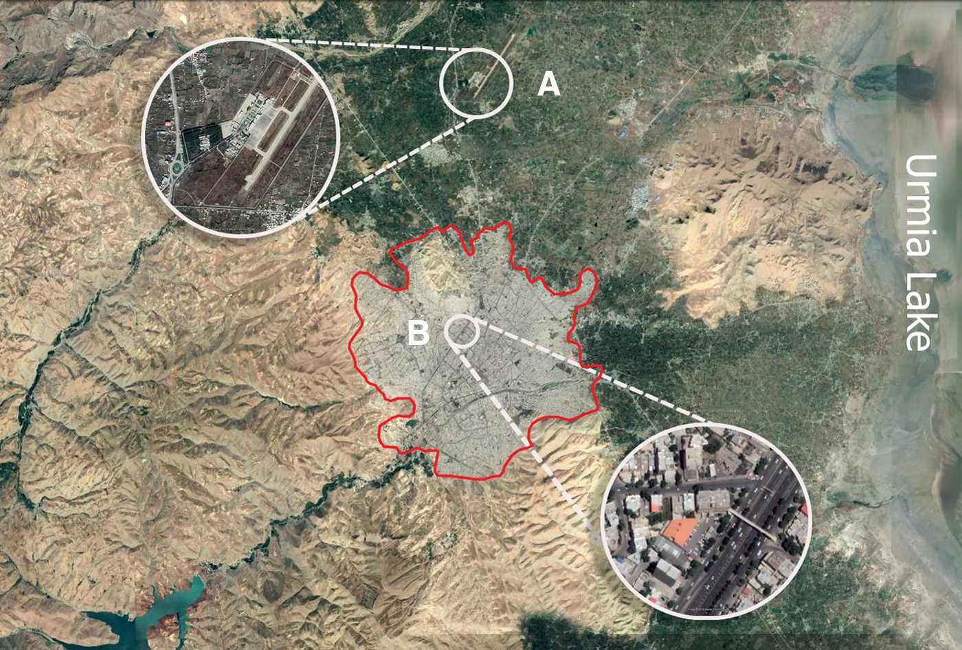
Location of air quality monitoring and meteorological station in the Urmia City. (A: Urmia airport synoptic station; B: Urmia air quality monitoring station No. 3; the red line represents the city of Urmia).

Research Method

Variables selection

To predict the concentrations of the indicator, air pollution parameter (PM_2.5, here), network input variables must be determined at first. Generally, model inputs can be selected according to prior information on the variables' characteristics as well as to past researches (Ordieres et al., 2005; Memarianfard and Hatami, 2017; Perez and Menares, 2018). We started with a large amount of candidate input parameters (air pollutants and meteorological variables). Only those that improved predicted PM_2.5 values were kept.

Statistical data were collected over a 2-year period (from December 9, 2016 to December 9, 2018). Air pollution data were obtained from Urmia air quality monitoring station No. 3. These data include concentrations of SO₂, CO, PM₁₀, PM_2.5, and NO₂ on an hourly basis. Meteorological variables, including relative humidity, wind velocity, and air temperature, were selected as the meteorological parameters. They were obtained from the Meteorological Organization of West Azerbaijan Province as every 3 h a day basis (Urmia Airport Synoptic Station). Given that the guidelines for the concentration of PM_2.5 in ambient air quality standards are based on the daily averages, all input parameters averaged as daily means to predict the concentration of PM_2.5. They were obtained using spreadsheet (MS Excel).

To investigate the effective time period of input parameters, we used three input data scenarios in prediction process. The first scenario includes data of seven studied parameters from 1 day before the forecasting day, the second scenario includes the data of 1 and 2 days before the forecasting day, and finally, the third scenario includes the data of the 1, 2, and 3 days before the forecasting day. The distinguishing factor in these three scenarios is the impact of individual air pollutants and meteorological parameters of the previous days on the prediction of the indicator air pollution parameter (PM_2.5) for the current day.

Preparation of statistical data

To optimize network training, statistical data were normalized according to Equation (3.1) from 0 to 1 following the initial processing. One of the advantages of normalization of the input data is that neuron weight changes are minimized during computation. $X_{n o r m} = \frac{(X - X_{m i n})}{(X_{m a x} - X_{m i n})}$ (3.1)

where X_norm is the normalized values of data X, and X_min and X_max are the minimum and maximum values of X dataset, respectively.

ANN technique

Neural networks consist of a large number of simple processor components called neurons. Together, the set of neurons form a layer. Generally, these layers are divided into three categories: input, hidden, and output layers—the input layer that distributes the data in the network, the hidden layer that processes the data, and the output layer that extracts the results for specific inputs (Moustris et al., 2010).

Different structures of ANN models have been used by the researchers. In this article, MLP, RBF, and GRNN models (see below for description) are discussed among other neural networks widely used in air pollution forecasting. In addition, the impact of PCA method on these models is evaluated.

To train and evaluate the neural networks, the data of 2 years (627 data) were divided into three groups, including training (425 data), validation (101 data), and test (101 data) data set. MATLAB R2019a was used for implementation of neural networks. For reliable evaluation of the networks, training, validation, and test data sets were selected randomly 100 times and the evaluation parameters were calculated in each round, and the average of those evaluation parameters for 100 times assessment would be provided.

Multi-layer perceptron

MLP is the most common and successful type of neural network architecture with feed-forward network (FFN) topologies (Ordieres et al., 2005). These networks consist of several layers (one input layer, one or more hidden layers, and one output layer), each containing several neurons (Fig. 2).

FIG. 2.

Illustration of MLP artificial neural network. MLP, multi-layer perceptron.

In this architecture, all neurons (X₁, X₂, …, X_i) of a single layer are fully connected to the next layer neurons by weighted interface elements (ω_ji, ω_kj). Each neuron calculates its inputs weighted sum (total weighted inputs) and a fixed value which is called bias (b_j, b_k) and then passes it through a linear or nonlinear transfer function to create the output. Interface elements transmit the output of neurons to the next layer neurons. MLPs are typically trained using a supervised training algorithm. In these training algorithms, when input is applied to the network, its output is compared to the target. Then, the learning rules used to adjust the weights and biases to approximate the network output to the desired output. The most common type of supervised training algorithm is the Error Back-Propagation Algorithm (Haykin, 1994). In its learning cycle, this training algorithm consists of two steps: the forward and the backward steps. In the forward step, a specific input presented to the network passes through different layers and stimulates them. Its effect propagates from one layer to the next. Finally, its output is created based on the weights and biases of the network. In the backward step, all the weights and biases of the network are adjusted according to a training algorithm. The training algorithm adjusts the weights and biases such that the difference between the desired output and the network output is minimized. This learning method is an iterative approach and will continue until the cessation criterion is met. In this study, the structure of MLP neural network includes an input layer, a hidden layer and one output layer. The number of neurons in the input layer depends on the number of variables used for forecasting the output variable. For MLP neural networks, one hidden layer with a large number of neurons usually yield good results (Bishop, 1995). The number of nodes in the hidden layer was determined by trial and error in the training phase. Therefore, we tested the number of nodes from 6 to 12. The best result was obtained with nine neurons on the hidden layer. Sigmoid function was used as the transfer function in the hidden layer, and Levenberg-Marquardt algorithm was used for training.

Radial basis function

Like MLP neural networks, RBF networks are suited for applications such as pattern discrimination and classification, interpolation, predication, forecasting, and process modeling (Ordieres et al., 2005). Both the MLP and RBF models are feed-forward neural networks (FFNN). A RBF is composed of an input layer, a hidden layer, and an output layer (Fig. 3). It uses RBFs as activation functions.

FIG. 3.

Illustration of RBF neural network. RBF, radial basis function.

The input layer sends input data (X₁, X₂, …, X_n) to each neuron of the hidden layer. These neurons (φ₁, φ₂, …, φ_k) transmit input signal through a transfer function. Typically, the activation function in the hidden layer is the Gaussian function [Eq. (3.2)]. $a_{j} (X) = e x p [- \frac{{∥X_{i} - c_{j}∥}^{2}}{2 {σ_{j}}^{2}}]$ (3.2)

where σ_j is the width of the jth neuron, X_i and c_j are the network input and the center of the hidden layer neuron, respectively, and || || denotes Euclidean distance algorithm. The output layer also consists of an arbitrary number of computational units that perform a linear combination of the RBFs computed by the hidden layer units.

The RBF neural network performance is based on spread value and maximum number of neurons in hidden layer. In this network, neurons were added sequentially to the hidden layer until the desired performance was obtained. In this study, we examined different numbers of hidden layer neurons and spread values. The best results were obtained based on σ_j = 0.4.

Generalized regression neural network

These networks fall into the category of probabilistic networks. Their advantages are fast learning, consistency, and optimal regression with large number of samples (Ren et al., 2010). A GRNN structure is composed of four layers: input layer, pattern layer, summation layer, and output layer (Fig. 4).

FIG. 4.

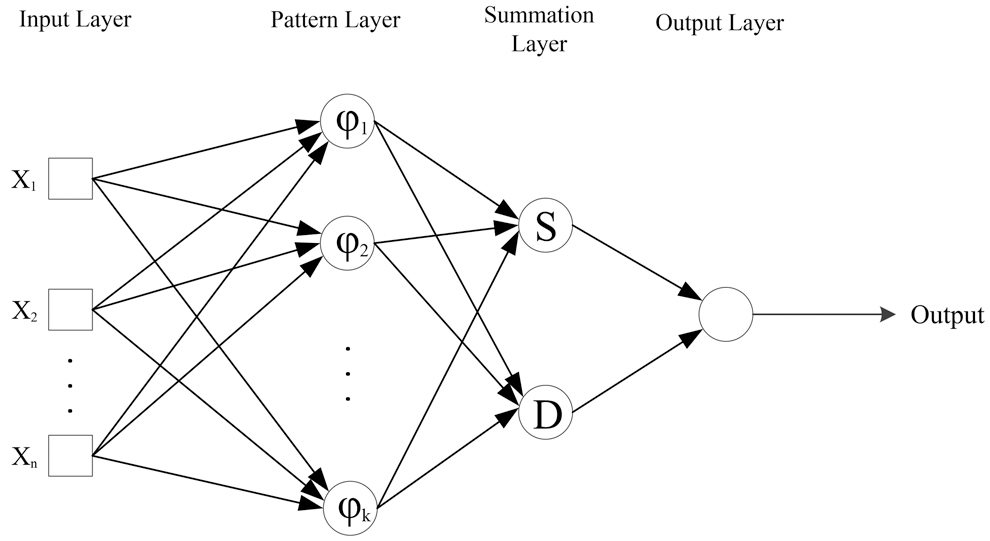
Illustration of GRNN. GRNN, generalized regression neural network.

The input layer is completely attached to the second layer (pattern layer). The input layer collects data and transmits them to the next layer (pattern layer). The pattern layer is used to perform clustering on the training process. Then information passes through summation layer. The summation layer consists of two neurons: S-Summation and D-Summation neuron. These two neurons are calculated according to Equation (3.3). Neuron S calculates the weighted sum of pattern layer outputs, while neuron D presents the nonweighted outputs of pattern layer neurons. The applied weight between a neuron in the pattern layer and the neuron S is the desired output of the training sample related to that neuron. In the case of neuron D, this value is equal to 1. The output layer divides the output of each neuron in the layer S by the output of the neuron D and obtains the final output of an unknown input vector [Eq. (3.4)]. $S = \sum_{i = 1}^{n} ω_{i} e x p [- D (X, X_{i})]$

D = \sum_{i = 1}^{n} e x p [- D (X, X_{i})]

(3.3)

Y (X) = \frac{S}{D} = \frac{\sum_{i = 1}^{n} ω_{i} e x p [- D (X, X_{i})]}{\sum_{i = 1}^{n} e x p [- D (X, X_{i})]}

(3.4)

where n is the number of training patterns and $ω_{i}$ is the weight of attaching the ith neuron of the pattern layer to the integration layer. The Gaussian function D is also defined as Equation (3.5). $D (X, X_{i}) = \sum_{j = 1}^{p} {[\frac{X_{j} - X_{i j}}{σ_{j}}]}^{2}$ (3.5)

where p represents the number of input layer elements, X_j and X_ij represent the jth element of X and X_i, respectively.

In GRNN model, the key parameter is ( $σ_{j}$ ), that is known as spread factor. Different spread factor values have been checked to find out the optimal spread value for predication of PM_2.5. In this study, we trained GRNN network with different ( $σ_{j}$ ) values in the Gaussian radial function. The best results were obtained based on σ_j = 0.1.

PCA method

PCA is among the multivariate statistical methods widely used in air pollution analysis (Sousa et al., 2007; Lu et al., 2011; Kumar and Goyal, 2013; Azid et al., 2014). The purpose of PCA is to reduce the number of predictor variables and convert them to new variables. Thereby, the initial variables (X_i) are transformed into new independent components (Z_i). These independent new variables illustrate different aspects of the initial variables. The newly created components are the result of a linear combination of the initial data [Eq. (3.6)]. $Z_{i} = {c_{i}}_{1} X_{1} + {c_{i}}_{2} X_{2} + \dots + c_{i n} X_{n}$ (3.6)

where Z_i is the new component, c_ij represents the coefficients of the initial variables (mapping), and X_i represents the initial variables. By solving [Eq. (3.7)], the coefficients of the initial variables (mapping) could be obtained. The mapping coefficients would be obtained from the covariance matrix eigenvectors. The components corresponding to the largest eigenvalue is considered as the best feature. Eigenvalues of the covariance matrix are obtained using the Equation (3.7). $| C - λ I | = 0$ (3.7)

where I is the identity matrix, λ is the eigenvalue, and | | indicates the determinant of the matrix. For each eigenvalue, an eigenvector is obtained using Equation (3.8) where v represents the eigenvector and is used as mapping coefficient. $C v = λ v$ (3.8)

Evaluation criteria

Since no neural network with a specific information architecture can generally be considered as the most appropriate network, networks need to be evaluated according to different criteria. In this article, the selection criteria for optimal architecture among the studied neural network models (i.e., MLP, RBF, and GRNN models) are minimum mean squared error (MSE), mean absolute error (MAE), and maximum correlation coefficient (R²) using Equations (3.9) to (3.11). $M S E = \frac{1}{N} \sum {(P_{i} - O_{i})}^{2}$ (3.9)

M A E = \frac{1}{N} \sum |P_{i} - O_{i}|

(3.10)

R^{2} = \frac{\sum_{i = 1}^{N} {[P_{i} - Ō]}^{2}}{\sum_{i = 1}^{N} {[O_{i} - Ō]}^{2}}

(3.11)

where N is the number of data points, O_i is the initial data, P_i is the prediction outcome, and $Ō$ is the mean of the initial data.

Results and Discussion

Investigating the effective time difference of input parameters in forecasting the PM_2.5 concentrations

All three scenarios were entered to the three MLP, RBF, and GRNN neural networks as inputs. The results are presented in Table 1. Examining the efficiency of three neural networks with three different input scenarios shows that the maximum correlation coefficient (R²) of 0.8038 between the actual values and the predicted outcomes was recorded by the input scenario No. 2. In addition, the minimum MSE and MAE were 110.1887 and 6.8454, respectively. Therefore, based on the results presented in Table 1, the RBF neural network with the second scenario inputs has the best performance in predicting PM_2.5 pollutant concentrations compared to other networks. This is consistent with the previous researchers (Ordieres et al., 2005; Yadav and Nath, 2018).

Table 1.

Performance Evaluation of Three Input Scenarios in Predicting PM_2.5 Concentration

Input data scenario	Values of evaluation criteria corresponding to each ANN model
	MSE			MAE			R²
	MLP	RBF	GRNN	MLP	RBF	GRNN	MLP	RBF	GRNN
Sc. #1	137.7545	137.8417	123.6249	7.2507	7.4851	7.0842	0.7710	0.7529	0.7787
Sc. #2	122.1435	110.1887	115.2296	7.1002	6.8454	6.9665	0.7845	0.8038	0.7949
Sc. #3	137.3746	117.4802	120.0242	7.6014	6.8558	7.0342	0.7521	0.7939	0.7757

ANN, artificial neural network; GRNN, generalized regression neural network; MAE, mean absolute error; MLP, multi-layer perceptron; MSE, mean squared error; RBF, radial basis function.

The comparison of the RBF neural network results for different input scenarios indicates that including the data of 2 days before the forecasting process into the first scenario has cased 6.76% improvement in the correlation coefficient (from 0.7529 for the first scenario to 0.8038 for the second scenario). However, a further increase in input data of the previous days (i.e., 3 days before the forecasting) resulted in a decrease of the correlation coefficient from 0.8038 for the second scenario to 0.7939 for the third scenario. In a study, Nouri et al. (2018) indicated that there is a significant relationship between PM_2.5 and NO₂ in Urmia city (with a Pearson coefficient of 0.85). It indicates that NO₂ has an effect on PM_2.5 concentrations. As shown in Fig. 5, the concentrations of PM_2.5 increased with the NO₂ concentrations (for more detail, please see Supplementary Table S2). Given the above findings, as well as the fact that most particles form in the atmosphere as a result of complex reactions of chemicals such as sulfur dioxide and nitrogen oxide, which are pollutants emitted from power plants, industries, and automobiles (U.S. EPA), they are called secondary particles. In the one hand, NO₂ is the main source of the nitrate aerosols, which form an important fraction of PM_2.5 (WHO, 2018), it is concluded that the changes of PM_2.5 and NO₂ concentration is basically synchronous. In addition, NO₂ is an important contributor to PM_2.5. Because of the low retention time of NO₂ in the atmosphere (1–2 days, Chang et al., 1979), the third scenario (including data of the last 3 days) fails to predict PM_2.5 concentrations. On the other hand, the lack of data for the network training in the first scenario could be the reason for the higher efficiency of the second scenario.

FIG. 5.

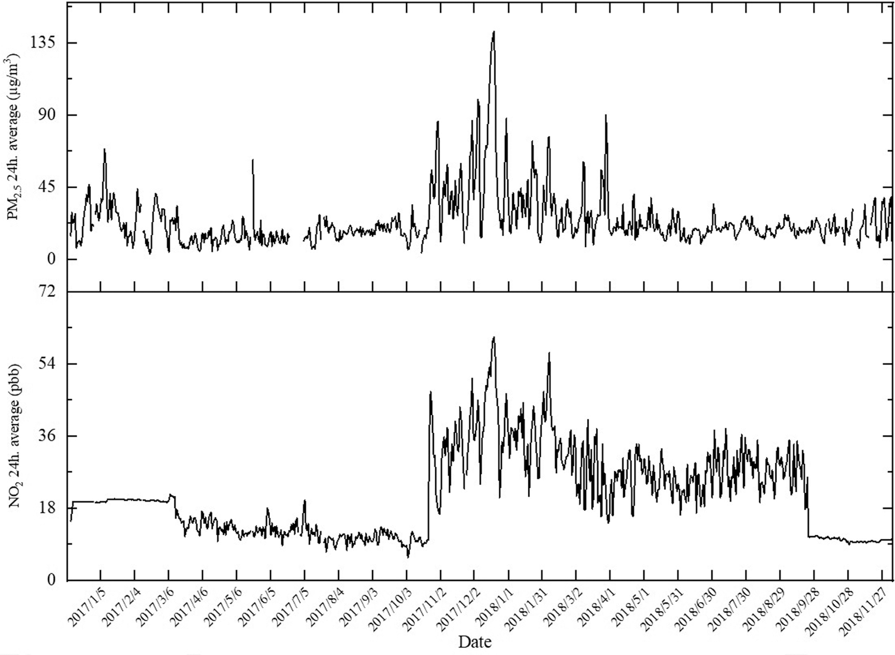
Daily mean concentrations of NO₂ and PM_2.5 during 2016–2018 period.

Investigation of the impact of the PCA approach on the efficiency of the three networks, MLP, RBF, and GRNN

Based on the results of Investigating the Effective Time Difference of Input Parameters in Forecasting the PM2.5 Concentrations section, the input data of the second scenario with the most efficiency in predicting PM_2.5 concentrations were selected as the network input. In the first step, all networks were executed without applying the PCA method. The results of the implementation of all neural networks based on three evaluation parameters, MSE, MAE, and R² are presented in Table 2. It should be noted that at this step, the values of the evaluation parameters are the average of network running for 100 times. As can be seen in Table 1 (or in the first row of Table 2), the maximum correlation coefficient (R²) for the network without applying the PCA was 0.8038. Furthermore, the minimum MSE and MAE values (110.19 and 6.84, respectively) were resulted from the RBF network.

Table 2.

Results of Evaluation Parameters for Three Multi-Layer Perceptron, Radial Basis Function, and Generalized Regression Neural Network Networks With/Without Applying Principal Component Analysis

Application of PCA method	Values of evaluation criteria corresponding to each ANN model
	MSE			MAE			R²
	MLP	RBF	GRNN	MLP	RBF	GRNN	MLP	RBF	GRNN
Without PCA	122.14	110.19	115.23	7.10	6.84	6.97	0.7845	0.8038	0.7949
With PCA	117.96	102.92	115.08	6.77	6.76	6.82	0.8145	0.8261	0.8060

PCA, principal component analysis.

In the second step, input variables were standardized and then, PCA method was applied to the data. According to the results presented in Table 2, it is shown that the effect of PCA method on the efficiency of all three networks is of incremental trend. MLP has the highest increase percentage based on the correlation coefficient parameter (3.8%) compared to the other networks (R² increased by 2.8% and 1.4% for RBF and GRNN networks, respectively). In other words, the application of the PCA method in the MLP network has increased the prediction accuracy by around 4%, which considered a significant value in forecasting the contaminants.

Then, the covariance matrix with 14 input parameters (equal to the number of input variables: 7 parameters of a day before the forecasting plus 7 parameters of 2 days before the forecasting) was formed. By applying the PCA technique, 14 new components as linear combinations of all the initial variables were obtained. The results of three evaluation parameters (based on testing values) were obtained for each MLP, RBF, and GRNN network by changing the number of input components (Table 3, a similar table using training values is presented in Supplementary Data, see Supplementary Table S1). According to Table 3, the features No. 1 to 8 (i.e., PC1 to 8) have the best efficiency in predicting PM_2.5 concentrations due to their desirable statistical index values. Therefore, it can be concluded—based on the above findings—that using PCA in the forecasting process made the network architecture simpler and faster (18.57 s without PCA and 18.04 s with PCA) despite a reduction in the number of input variables from 14 parameters to 8 new components. In addition, no effect of all main variables in the prediction process was ignored. It was because the components created by this method are linear combinations of all variables.

Table 3.

Performance evaluation of Principal Component

No. of features	Values of evaluation criteria corresponding to each ANN model
	MSE			MAE			R²
	MLP	RBF	GRNN	MLP	RBF	GRNN	MLP	RBF	GRNN
1	397.9947	2847838	269.8886	10.515	1453	10.166	0.4069	0.2740	0.4495
2	224.0328	2345527	191.8973	9.0931	846.29	8.8661	0.6027	0.2975	0.6308
3	145.2343	2413418	153.2764	7.6356	67.291	7.9930	0.7529	0.3083	0.7337
4	126.5696	211.6380	135.9600	7.2138	8.6838	7.5079	0.7881	0.6410	0.7685
5	123.6344	179.4767	148.8940	7.2285	8.4437	7.7262	0.7823	0.6987	0.7370
6	135.9509	168.4331	159.2728	7.2707	8.2088	7.6895	0.7606	0.7062	0.7116
7	213.2292	124.5780	131.0052	7.0887	7.3711	7.1478	0.7833	0.7836	0.7658
8	117.9572	102.9213	115.5819	6.7697	6.7628	6.8223	0.8145	0.8261	0.8060
9	125.8251	112.8341	127.2213	7.0255	6.8923	7.0842	0.7706	0.7816	0.7612
10	137.5989	107.7752	120.3011	7.1209	6.8339	7.0453	0.7846	0.8035	0.7791
11	134.2504	108.2325	126.5810	7.2200	6.8500	7.1631	0.7734	0.7976	0.7625
12	129.1865	110.4088	131.8695	7.2474	6.8540	7.2577	0.7918	0.8123	0.7767
13	133.0979	118.3277	133.3781	7.4566	7.0547	7.2984	0.7863	0.8064	0.7774
14	165.9979	119.3444	130.2254	7.5608	7.0799	7.3141	0.7600	0.7844	0.7663

Given the positive role of PCA approach in neural networks proved in previous research (Lu et al., 2004; Sousa et al., 2007), the results of this study also confirm the effect of PCA approach on ANNs.

Conclusions

Air pollution control, as one of the environmental science branches has gained the attention because of the potential for adverse effects on human health and interference with the comfortable and safe use of the environment, both at local and global levels. Hence, the prediction of the pollutants concentration is essential to take the necessary measures for reducing their harmful effects. The present study attempts to provide a precise model to forecast PM_2.5 concentrations. For this purpose, three different models of neural networks were studied. To investigate the effect of time difference on each input parameter, three input scenarios were defined for each neural network. Then, the impact of using the PCA approach on each neural network was evaluated. The following results are obtained in this study:

The RBF neural network with the second scenario inputs showed the best efficiency in forecasting PM_2.5 concentrations compared to other networks (MLP and GRNN). The highest correlation coefficient (R²) between the actual and the predicted outcomes is 0.8038.

The influence of input variables, including meteorological variables and air pollution data of 1 and 2 days before forecasting the PM_2.5 concentrations of the current day, was considerable on neural network efficiency.

Due to the NO₂ low retention time in the atmosphere (1–2 days) and to the fact that NO₂ is the major source of nitrate aerosols as an important part of PM_2.5, the data from 3 days before forecasting PM_2.5 concentrations showed inefficiency.

The small amount of information for training the network may be the reason for inefficiency of the first scenario.

Results of applying PCA method on each neural network showed that based on the correlation coefficient parameter (3.8%), MLP network had the highest increase percentage.

Although the PCA method did not have a significant effect on increasing the prediction accuracy, its main advantage is to reduce the number of input parameters, while all main parameters were involved in the prediction process.

Footnotes

Acknowledgment

The authors acknowledge Mr. Saeed Mousavi Moughanjogi, expert of West Azerbaijan Environmental Protection Organization, for his valuable supports throughout this research performance.

Author Disclosure Statement

The authors declare that there is no conflict of interests regarding the publication of this article. In addition, the ethical issues, including plagiarism, informed consent, misconduct, data fabrication and/or falsification, double publication and/or submission, and redundancy, have been completely observed by the authors.

Funding Information

No funding was received for this study.

Supplementary Material

References

Azid

, Juahir

, Toriman

M.E.

, Kamarudin

M.K.A.

, Saudi

A.S.M.

, Hasnam

C.N.C.

, Aziz

NAA

, Azaman

, Latif

, Zainuddin

SFM

, and Osman

M.R.

(2014). Prediction of the level of air pollution using principal component analysis and artificial neural network techniques: A case study in Malaysia. Water Air Soil Pollut. 225, 2063.

Banja

, Papanastasiou

D.K.

, Poupkou

, and Melas

(2012). Development of a short-term ozone prediction tool in Tirana area based on meteorological variables. Atmos. Pollut. Res. 3, 32.

Bishop

C.M.

(1995). Neural Networks for Pattern Recognition. Great Britain: Oxford University Press.

Brook

R.D.

, Brook

J.R.

, Urch

, Vincent

, Rajagopalan

, and Silverman

(2002). Inhalation of fine particulate air pollution and ozone causes acute arterial vasoconstriction in healthy adults. Circulation, 105, 1534.

Brzozowska

(2013). Validation of a Lagrangian particle model. Atmos. Environ. 70, 218.

Chang

T.Y.

, Norbeck

JM.

, and Weinstock

(1979). An estimate of the NOx removal rate in an urban atmosphere. Environ. Sci. Tech. 13, 1534.

Collett

R.S.

, and Oduyemi

(1997). Air quality modelling: A technical review of mathematical approaches. Meteorol. Appl. 4, 235.

Cortina-Januchs

M.G.

, Quintanilla-Dominguez

, Vega-Corona

, and Andina

(2015). Development of a model for forecasting of PM10 concentrations in Salamanca, Mexico. Atmos. Pollut. Res. 6, 626.

D'Amico

, Petroni

, and Prattico

(2014). Wind speed and energy forecasting at different time scales: A nonparametric approach. Phys. A Stat. Mech. Appl. 406, 59.

10.

Fernando

H.J.

, Mammarella

M.C.

, Grandoni

, Fedele

, Di Marco

, Dimitrova

, and Hyde

(2012). Forecasting PM10 in metropolitan areas: Efficacy of neural networks. Environ. Pollut. 163, 62.

11.

Franceschi

, Cobo

, and Figueredo

(2018). Discovering relationships and forecasting PM10 and PM2. 5 concentrations in Bogotá, Colombia, using artificial neural networks, principal component analysis, and k-means clustering. Atmos. Pollut. Res., 9, 912.

12.

Gao

, Zhao

, Bai

, Han

, Xu

, Zhao

, Zhang

, Chen

, Lei

, Shi

, Zhang

, Li

, and Yu

(2020). Combined use of principal component analysis and artificial neural network approach to improve estimates of PM_2.5 personal exposure: A case study on older adults. Sci. Total Environ. 726, 138533.

13.

Grivas

, and Chaloulakou

(2006). Artificial neural network models for prediction of PM10 hourly concentrations, in the Greater Area of Athens, Greece. Atmos. Environ. 40, 1216.

14.

Haykin

(2007). Neural networks: a comprehensive foundation. Prentice-Hall, Inc., USA.

15.

Holmes

N.S.

, and Morawska

(2006). A review of dispersion modelling and its application to the dispersion of particles: An overview of different dispersion models available. Atmos. Environ. 40, 5902.

16.

Hrust

, Klaić

Z.B.

, Križan

, Antonić

, and Hercog

(2009). Neural network forecasting of air pollutants hourly concentrations using optimised temporal averages of meteorological variables and pollutant concentrations. Atmos. Environ. 43, 5588.

17.

Ibarra-Berastegi

, Elias

, Barona

, Saenz

, Ezcurra

, and de Argandoña

J.D.

(2008). From diagnosis to prognosis for forecasting air pollution using neural networks: Air pollution monitoring in Bilbao. Environ. Model. Softw. 23, 622.

18.

Jerrett

, Arain

, Kanaroglou

, Beckerman

, Potoglou

, Sahsuvaroglu

, Morrison

, and Giovis

(2005). A review and evaluation of intraurban air pollution exposure models. J. Expo. Sci. Environ. Epidemiol. 15, 185.

19.

Jorquera

(2002). Air quality at Santiago, Chile: A box modeling approach—I. Carbon monoxide, nitrogen oxides and sulfur dioxide. Atmos. Environ., 36, 315.

20.

Jung

C.R.

, Lin

Y.T.

, and Hwang

B.F.

(2015). Ozone, particulate matter, and newly diagnosed Alzheimer's disease: A population-based cohort study in Taiwan. J Alzheimer's Dis. 44, 573.

21.

Kim

K.H.

, Kabir

, and Kabir

(2015). A review on the human health impact of airborne particulate matter. Environ. Int. 74, 136.

22.

Klemm

R.J.

, Mason, Jr

R.M.

, Heilig

C.M.

, Neas

L.M.

, and Dockery

D.W.

(2000). Is daily mortality associated specifically with fine particles? Data reconstruction and replication of analyses. J. Air Waste Manage. Assoc. 50, 1215.

23.

Kukkonen

, Partanen

, Karppinen

, Ruuskanen

, Junninen

, Kolehmainen

, Niska

, Dorling

, Chatterton

, Foxall

, and Cawley

(2003). Extensive evaluation of neural network models for the prediction of NO2 and PM10 concentrations, compared with a deterministic modelling system and measurements in central Helsinki. Atmos. Environ. 37, 4539.

24.

Kumar

, and Goyal

(2013). Forecasting of air quality index in Delhi using neural network based on principal component analysis. Pure Appl. Geophys. 170, 711.

25.

W.Z.

, He

H.D.

, and Dong

L.Y.

(2011). Performance assessment of air quality monitoring networks using principal component analysis and cluster analysis. Build. Environ. 46, 577.

26.

W.Z.

, Wang

W.J.

, Wang

X.K.

, Yan

S.H.

, and Lam

J.C.

(2004). Potential assessment of a neural network model with PCA/RBF approach for forecasting pollutant trends in Mong Kok urban air, Hong Kong. Environ. Res. 96, 79.

27.

Martins

N.R.

, and da Graça

G.C.

(2018). Impact of PM_2.5 in indoor urban environments: A review. Sustain. Cities Soc. 42, 259.

28.

McHenry

J.N.

, Ryan

W.F.

, Seaman

N.L.

, Coats, Jr

C.J.

, Pudykiewicz

, Arunachalam

, and Vukovich

J.M.

(2004). A real-time Eulerian photochemical model forecast system: Overview and initial ozone forecast performance in the northeast US corridor. Bull. Am. Meteorol. Soc. 85, 525.

29.

Memarianfard

, and Hatami

A.M.

(2017). Artificial neural network forecast application for fine particulate matter concentration using meteorological data. Global J. Environ. Sci. Manage. 3, 333.

30.

Moustris

K.P.

, Ziomas

I.C.

, and Paliatsos

A.G.

(2010). 3-day-ahead forecasting of regional pollution index for the pollutants NO2, CO, SO2, and O3 using artificial neural networks in Athens, Greece. Water Air Soil Pollut. 209, 29.

31.

Nouri

, Ghanbarzade lak

, and Mosavi Moghanjogi

(2018). Investigation of the source of air poiiution crisis in Urmia city in December 2017. 1ST National Conference on Infrastructure Engineering, Urmia University. (in Persian)

32.

Ordieres

J.B.

, Vergara

E.P.

, Capuz

R.S.

, and Salazar

R.E.

(2005). Neural network prediction model for fine particulate matter (PM2. 5) on the US-Mexico border in El Paso (Texas) and Ciudad Juárez (Chihuahua). Environ. Model. Softw., 20, 547.

33.

Perez

, and Menares

(2018). Forecasting of hourly PM2. 5 in south-west zone in Santiago de Chile. Aerosol Air Qual. Res., 18, 2666.

34.

Perez

, and Reyes

(2001). Prediction of particulate air pollution using neural techniques. Neural Comput Appl. 10, 165.

35.

Perez

, and Salini

(2008). PM2. 5 forecasting in a large city: Comparison of three methods. Atmos. Environ., 42, 8219.

36.

Pérez

, Trier

, and Reyes

(2000). Prediction of PM2. 5 concentrations several hours in advance using neural networks in Santiago, Chile. Atmos. Environ., 34, 1189.

37.

Pope

III

, C.A., Burnett

R.T.

, Thun

M.J.

, Calle

E.E.

, Krewski

, Ito

, and Thurston

G.D.

(2002). Lung cancer, cardiopulmonary mortality, and long-term exposure to fine particulate air pollution. JAMA, 287, 1132.

38.

Ren

, Yang

, Ji

, and Tian

(2010). Application of generalized regression neural network in prediction of cement properties. In 2010 International Conference on Computer Design and Applications, Vol. 2. Qinhuangdao, China: IEEE, pp. V2–V385.

39.

Schwartz

, and Neas

L.M.

(2000). Fine particles are more strongly associated than coarse particles with acute respiratory health effects in schoolchildren. Epidemiology, 11, 6.

40.

Sharma

, Chandra

, and Kaushik

S.C.

(2009). Forecasts using Box–Jenkins models for the ambient air quality data of Delhi City. Environ. Monit. Assess. 157, 105.

41.

Shi

J.P.

, and Harrison

R.M.

(1997). Regression modelling of hourly NOx and NO2 concentrations in urban air in London. Atmos. Environ. 31, 4081.

42.

Spurny

K.R.

(1998). On the physics, chemistry and toxicology of ultrafine anthropogenic, atmospheric aerosols (UAAA): New advances. Toxicol. Lett. 96, 253.

43.

Sousa

S.I.V.

, Martins

F.G.

, Alvim-Ferraz

M.C.M.

, and Pereira

M.C.

(2007). Multiple linear regression and artificial neural networks based on principal components to predict ozone concentrations. Environ. Model. Softw. 22, 97.

44.

Wang

J.F.

, Hu

M.G.

, Xu

C.D.

, Christakos

, and Zhao

(2013). Estimation of citywide air pollution in Beijing. PLoS One, 8, e53400.

45.

World Health Organization (WHO). (2018). Ambient (outdoor) air quality and health, Key Facts. Available at (accessed on September, 2019): https://www.who.int/en/news-room/fact-sheets/detail/ambient-(outdoor)-air-quality-and-health (accessed September, 2019).

46.

Yadav

, and Nath

(2018). Daily prediction of PM 10 using radial basis function and generalized regression neural network. In 2018 Recent Advances on Engineering, Technology and Computational Sciences (RAETCS). Allahabad, India: IEEE, pp. 1–5.

Supplementary Material

Please find the following supplemental material available below.

For Open Access articles published under a Creative Commons License, all supplemental material carries the same license as the article it is associated with.

For non-Open Access articles published, all supplemental material carries a non-exclusive license, and permission requests for re-use of supplemental material or any part of supplemental material shall be sent directly to the copyright owner as specified in the copyright notice associated with the article.

0.00 MB

0.21 MB

0.30 MB

Prediction of PM 2.5 Concentrations Using Principal Component Analysis and Artificial Neural Network Techniques: A Case Study: Urmia,Iran

Abstract

Introduction

Study Area

Research Method

Variables selection

Preparation of statistical data

ANN technique

Multi-layer perceptron

Radial basis function

Generalized regression neural network

PCA method

Evaluation criteria

Results and Discussion

Investigating the effective time difference of input parameters in forecasting the PM2.5 concentrations

Investigation of the impact of the PCA approach on the efficiency of the three networks, MLP, RBF, and GRNN

Conclusions

Footnotes

Acknowledgment

Author Disclosure Statement

Funding Information

Supplementary Material

References

Supplementary Material

Investigating the effective time difference of input parameters in forecasting the PM_2.5 concentrations