Groundwater Pollution Sources Identification Based on Hybrid Homotopy-Genetic Algorithm and Simulation Optimization

Abstract

Genetic algorithm (GA) is often used to solve the optimization model of groundwater pollution source identification. However, GA is prone to premature convergence and fall into local optimum. Thus, homotopy algorithm and GA are used in combination to improve the disadvantage. Then hybrid homotopy-genetic algorithm (HGA) was applied to solve the optimization model. A 0–1 mixed integer nonlinear optimization model (0–1MINLP) based on kriging surrogate model was used to simultaneously identify hydraulic conductivity, location, and release history of pollution sources. The results showed that the 0–1MINLP based on a kriging surrogate model could simultaneously identify the hydraulic conductivity and information of pollution sources, while maintaining a certain level of precision and reducing calculation load. The combination of homotopy algorithm and GA can improve the shortcomings of GA that is easy to fall into premature convergence. The identification results obtained by the HGA were closer to the true values of the pollution source characteristics compared with GA.

Introduction

Groundwater is located underground, and thus groundwater pollution is generally characterized by concealment and a delay before its discovery. As a consequence, there is a poor understanding of the status of groundwater pollution sources, including the number, location, and release history of groundwater pollution sources in aquifers, which can hinder the design of groundwater pollution remediation schemes, risk assessments, and determining liability for pollution (Snodgrass and Kitanidis, 1997; Lapworth et al., 2012). Therefore, investigating the identification for groundwater pollution is particularly important.

Groundwater pollution source identification (GPSI) is based on measured groundwater pollution values as well as auxiliary information obtained from field investigations and professional experience. Solving numerical simulation models of groundwater pollution using various mathematical methods can identify relevant information about the groundwater pollution sources in aquifers, including the number, location, and release history (the release history refers to the release intensity of contaminants in each period) (Sun et al., 2006).

Effective GPSI can provide the basic conditions for the rational formulation of a groundwater pollution remediation plan, pollution risk assessments, and determining the liability for pollution. Thus, it has important theoretical significance and possible practical applications (Bagtzoglou and Atmadja, 2005).

The problem of GPSI was formulated in the 1980s. Gorelick et al. (1983) identified the location and release intensity of groundwater pollution sources by using least squares regression and linear programming. Mahar and Datta (2000) proposed a identification method for GPSI based on a nonlinear optimization model, and they studied the effects of the relative locations of observations on the identification accuracy. Mahinthakumar and Sayeed (2005) applied a genetic algorithm-local search (GA-LS) method to identify the location and release intensity of groundwater pollution sources. Their results showed that the identification results obtained using the GA-LS method were better than those produced with a single GA method or a local search method. Sun et al. (2006) used a constrained robust least squares method to identify the release history for pollution sources. Singh and Datta (2007) used an artificial neural network model to identify the release intensity of groundwater pollution sources and the missing concentration data for pollutants. Mirghani et al. (2009) used a parallel evolutionary search strategy to solve the simulation optimization model for a groundwater pollution source and identified the location and initial release intensity of the pollution source. Ayvaz (2010) embedded the MODFLOW and MT3DMS simulation models in an optimization model, and then used the heuristic harmony search algorithm to solve the optimization model to identify the number, location, and release history of pollution sources. Tamer Ayvaz (2016) used a combination of a GA and generalized simplified gradient algorithm to identify the location and release intensity of groundwater pollution source.

GA is a heuristic search method and is often used to solve the optimization model of GPSI. However, the GA is affected by the risk of premature convergence (An et al., 2009; Guo and Zhou, 2009). Therefore, it is important to improve the problem of GA in terms of premature convergence and fall into local optimum. The GA needs to initialize the population at the beginning of the iteration. The initialization methods of the population include random method and fixed value setting method. Using random methods to generate initial population cannot control the quality of initial population. The selection of the initial population for the GA will affect the identified result of the optimization problem. If the initial population is far from the true value, the algorithm is affected by the risk of premature convergence and the real pollution source information is not obtained. Thus, combining the homotopy algorithm with the GA and applying the homotopy method to generate the initial population (fixed value setting method) for the GA through path tracking can make the initial population more appropriate. Thus, combining the homotopy algorithm with GA can improve the disadvantages of premature convergence (fall into local optimum) for GA.

The simulation optimization method is used to perform GCSI in this study. A 0–1MINLP was established to simultaneously identify the hydraulic conductivity, location, and release history of pollution sources. The surrogate model of the simulation model was linked to 0–1MINLP to reduce the calculation load and time required when solving the optimization model while ensuring the inversion accuracy (Xing et al., 2019). The homotopy-genetic algorithm (HGA) was used to solve the 0–1MINLP, thereby preventing GA itself becoming trapped by a local optimal solution.

Methodology

In this study, the hydraulic conductivity, location and release history of pollution sources were identified based on simulation-optimization method.

Homotopy algorithm

Many studies have considered the existence and effective solutions of nonlinear equations, but these methods have an inevitable shortcoming because whether they can search for the optimal solution of the optimization problem has a certain relationship with the choice of the initial population. If the appropriate initial population is not selected at the beginning of the iteration process, the optimal solution may not be obtained (Puangdownreong et al., 2004; Bei, 2014). However, for most nonlinear equations, it is difficult to find appropriate initial population, which can make it difficult or impossible to solve the nonlinear problem. The homotopy algorithm is a method for obtaining the solutions of nonlinear equations, and it has previously been applied to topology problems in the field of algebra. Due to the complexity of the nonlinear system, the traditional solution method often has difficulty obtaining the exact solutions for the equations that need to be solved. Thus, a system of equations is constructed, which are simple to solve. The path track is finally obtained by solving these simple equations. Finding a solution for the system of equations is the basic idea of the homotopy algorithm (Garrigues and Ghaoui, 2008). This method imposes no strict limit on the initial population and it requires a small amount of calculations. This simple algorithm has a high success rate (Watson and Wang, 1981). The principle of the homotopy algorithm is as follows: $\{\begin{matrix} F (X) = {(f_{1} (x), f_{2} (x), f_{3} (x), \dots f_{n} (x))}^{T} i = 1, 2, 3, \dots n \\ f_{i} (x) = f (x_{1}, x_{2} \dots x_{n}) x = (x_{1}, x_{2} \dots x_{n}) \in R^{n} \\ F (x) = 0 \end{matrix},$ (1) $\{\begin{matrix} G (X) = {(g_{1} (x), g_{2} (x), g_{3} (x), \dots g_{n} (x))}^{T} i = 1, 2, 3, \dots n \\ g_{i} (x) = g (x_{1}, x_{2} \dots x_{n}) x = (x_{1}, x_{2} \dots x_{n}) \in R \\ G (x) = 0 \end{matrix},$ (2)

\{\begin{matrix} H (X, λ) = λ G (X) + (1 - λ) F (X) λ = [0, 1] \\ H (X, 0) = F (X) \\ H (X, 1) = G (X) \end{matrix} .

(3)

where $F (X) = 0$ is a nonlinear equation with known solutions, $G (x) = 0$ is a nonlinear equation with unknown solutions, $λ$ is a homotopy parameter, and $H (X, λ)$ is a cluster of homotopy nonlinear equations constructed for $F (x)$ and $G (x)$ by applying the linear homotopy concept.

$λ$ changes from 0 to 1, so the solution of the homotopy nonlinear equations changes from the solution of $F (x)$ to the solution of $G (x)$ . By constructing a linear homotopy nonlinear equation, the solution of the unknown nonlinear equations is transformed into solving a cluster of homotopy nonlinear equations by starting from a simple solution and finally obtaining the solutions of the nonlinear equations by path tracking.

Genetic algorithm

GA is an optimization method for random global search, which mimics the evolutionary mechanism of biological evolution in nature (Zwickl, 2008). In this algorithm, a new population is generated that is more adaptable to the environment than the previous group by applying random genetic operators such as selection, crossover, and mutation to an arbitrarily selected initial population (Guo et al., 2018). After evolution for several generations, the new population gradually evolves into better areas of the search space. Finally, the population converges until it is the best adapted to the environment and this individual is the optimal solution to the problem. The principle of GA is detailed in Guo et al. (2018) article. The GA is simply explained as follows.

(1)

Coding: Before the GA performs the search, the solution to the actual problem is converted into binary data called code.

(2)

Generating the initial population: The evolution algebra counter and maximum evolution algebra are set, and M individuals are randomly generated as the initial population P(0).

(3)

Fitness evaluation test: The fitness function is defined according to the specific practical problem and the fitness is calculated for each of the individuals in the group P(t).

(4)

Evolution: The selection operator, crossover operator, and mutation operator are applied to the group. The group P(t) is selected, crossed, and mutated to obtain the next generation P(t + 1).

(5)

Termination condition judgment: If $t \leq T$ , then t + 1 replaces t and go to step (2). If $t > T$ , then the individual with the greatest fitness obtained during the evolution process is used as the optimal solution output and the operation is terminated.

Kriging method

The kriging method is an interpolation method proposed by the Georges Matheron. The kriging method was applied to establish a surrogate model in recent years (Hemker et al., 2008; Coetzee et al., 2012; Guo et al., 2018). The principle of kriging method was as follows: $Y (x) = \sum_{i = 1}^{p} β_{i} f_{i} (x) + Z (x)$ (4)

where $f (x)$ is determinate regression functions, $β$ is the coefficient of the corresponding regression functions, $p$ is the number of determinate regression function, and $Z (x)$ is Gaussian random function, and $Z (x)$ satisfies the following conditions: $\{\begin{matrix} E (Z (x)) = 0 \\ D (Z (x)) = σ^{2} \\ c o v (Z (x_{i}), Z (x_{j})) = σ^{2} R (θ, x_{i}, x_{j}) \end{matrix}$ (5) $R (θ, x_{i}, x_{j}) = exp (- \sum_{i = 1}^{n} θ_{k} {|x_{i}^{k} - x_{j}^{k}|}^{p_{k}})$ (6)

where R is the spatial correlation function matrix, θ denotes the correlation parameter, n denotes the number of dimensions in the set of design variables, $x_{i}^{k}$ is the k-dimensional coordinate of the ith sample, and $p_{k}$ is undetermined coefficient.

Based on the input and output data for the n known sample points, the output value corresponding to any point x in the predicted feasible domain is: $Y (x) = f^{T} β^{*} + r^{T} (x) R^{- 1} (y - f β^{*})$ (7)

R = [\begin{matrix} \begin{matrix} R (x_{1}, x_{1}) & \dots & R (x_{1}, x_{n}) \\ ⋮ & ⋱ & ⋮ \\ R (x_{n}, x_{1}) & \dots & R (x_{n}, x_{n}) \end{matrix} \end{matrix}]

(9)

where r(x) is the correlation vector of the point x and n sampling points is the matrix $n \times m, n$ is the number of sampling points, m is the dimension of the output value, R is a correlation matrix comprising the correlation coefficients of n sampling points, and $β^{*}$ is the undetermined coefficient of the linear regression part, which can be obtained with the optimal linear unbiased estimation.

The variance estimate value $σ^{2}$ is determined as follows.

{max}_{θ_{k}} \{- [n ln σ^{2} + ln |R|]\}

(11)

The surrogate model can be established by solving the nonlinear unconstrained optimization problem defined above. After obtaining the undetermined parameters $θ_{k}$ , the response value can be produced with the established surrogate model. $θ_{k}$ can be obtained with the unconstrained optimization formula (11) (Xu et al., 2007).

Method application

Site overview

The study considered two hypothetical cases. The advantage of a hypothetical case is that it does not require much time to study the complex conditions in the actual problem, thereby decreasing the time needed to identify and verify the simulation model. Moreover, it is possible to test the identified results.

Case 1 is a situation that many scholars have used (shown in Fig. 1a), which involves irregular geometry, inhomogeneous media, and transient flow (Ayvaz, 2010; Xing et al., 2019). Case 2 is a two-dimensional heterogeneous isotropic phreatic aquifer model with an irregular boundary. Three parameter partitions were defined (shown in Fig. 1b). The movement in the phreatic aquifer was transient flow. The vertical direction of the study area received uniform recharge of atmospheric rainfall with a recharge amount of 680 mm/a. Four pollution sources were present in the study area. The total simulation time for pollutant transport was 16 months and divided into eight stress periods (the computational time intervals for a MODFLOW simulation are called “stress periods”). Each stress period contained 2 months. Pollutant was released from the source within 8 months of the first four stress periods. Five observation wells were located in the study area.

FIG. 1.

(a) Hypothetical aquifer model for case 1. (b) Hypothetical aquifer model for case 2.

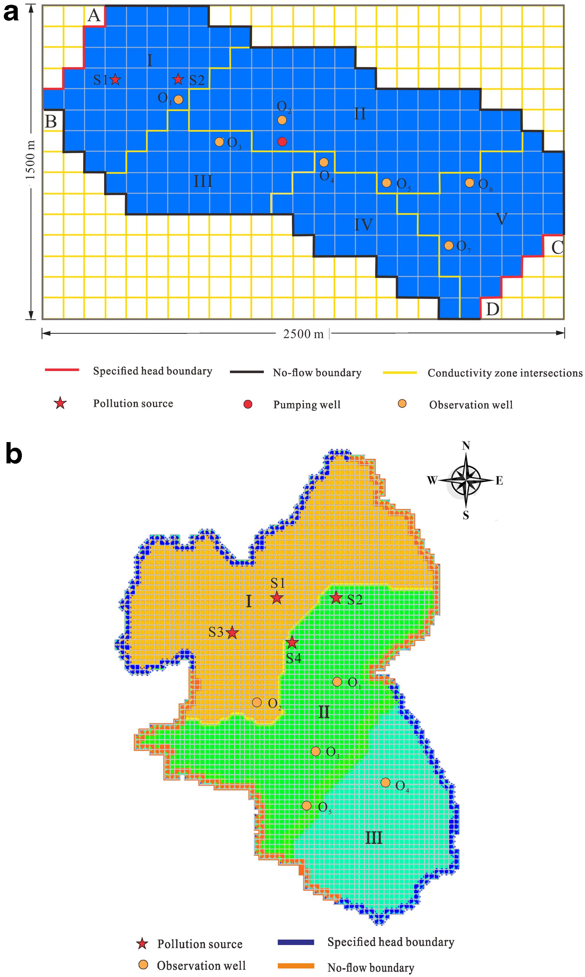
The boundary conditions and other related parameters for the two cases are listed in Tables 1 and 2, respectively. The initial concentration of the pollutants and the release intensities of the sources in for two cases are shown in Tables 3 and 4, respectively.

Table 1.

Aquifer Parameters for Case 1

Parameters values	I	II	III	IV	V
Hydraulic conductivity, K (m/d)	34.56	8.64	17.28	25.92	46.2
Specific yield, μ	0.25	0.16	0.18	0.20	0.30
Effective porosity, n	0.25	0.16	0.18	0.20	0.30
Volume flux per unit area, Q (m/d)	0.0000864
Longitudinal dispersivity, α_L (m)	40
Transverse dispersivity, α_T (m)	9.6
Initial concentration (mg/L)	100
Grid spacing in x-direction, Δx (m)	100
Grid spacing in y-direction, Δy (m)	100
Saturated thickness, b (m)	30.5

Table 2.

Aquifer Parameters for Case 2

Parameters values	I	II	III
Hydraulic conductivity, K (m/s)	0.00048	0.00032	0.00024
Specific yield, μ	0.29	0.25	0.21
Effective porosity, n	0.3	0.26	0.22
Volume flux per unit area, Q (m/d)	0.000372	0.000328	0.000276
Longitudinal dispersivity, α_L (m)	42	36	30
Transverse dispersivity, α_T (m)	8.4	7.2	6
Initial concentration (mg/L)	0.2	0.2	0.2
Grid spacing in x-direction, Δx (m)	8
Grid spacing in y-direction, Δy (m)	8
Saturated thickness, b (m)		42

Table 3.

Pollution Source Release Intensities in the Four Release Periods for Case 1

Pollution source	Release intensity of pollution source at each period (g/d × 10⁵)
Pollution source	SP1	SP2	SP3	SP4
S1	74.56	56.22	38.66	21.12
S2	54.44	47.5	33.65	23.64

Table 4.

Pollution Source Release Intensities in the Four Release Periods for Case 2

Pollution source	Release intensity of pollution source at each period (g/d × 10⁵)
Pollution source	SP1	SP2	SP3	SP4
S3	13	20	12	9
S4	26	33	18	14

The application of the identification method is shown in Fig. 2.

FIG. 2.

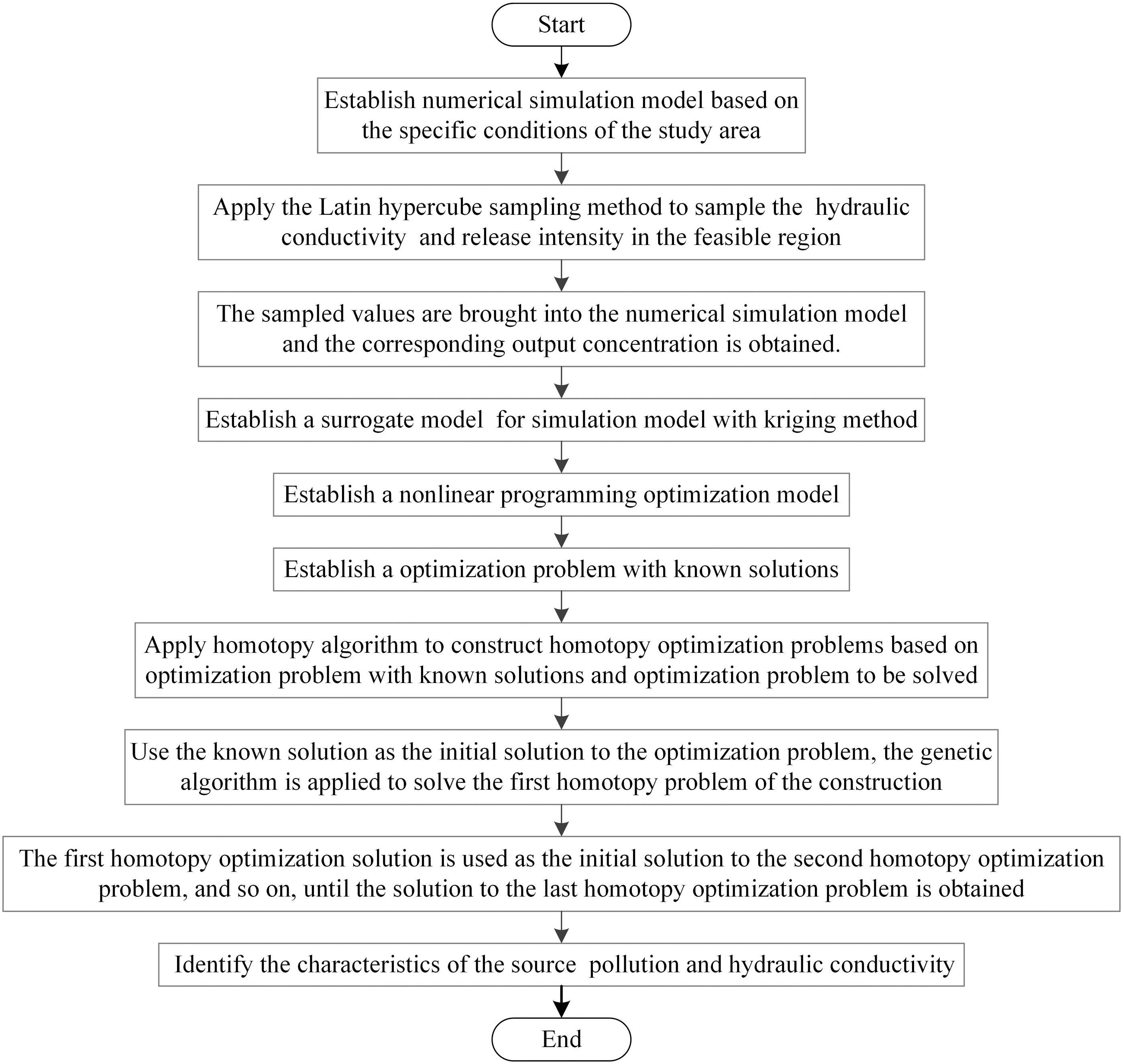
Application of the proposed method to the case study.

Numerical simulation model

The numerical simulation models of the groundwater flow and pollutant transport migration for case 1 and case 2 were established based on the specific conditions in the area. The governing partial differential equation for the transient flow in a two-dimensional aquifer system according to Darcy's law and the water balance principle can be given as follows: (Singh and Datta, 2007): $\frac{\partial}{\partial x_{i}} (K_{i j} \frac{\partial H}{\partial x_{j}}) + W = μ \frac{\partial H}{\partial t} i, j = 1, 2,$ (12)

where K_ij is the hydraulic conductivity, H is the hydraulic head, W is the volumetric flux per unit volume, and x are the Cartesian coordinates. $μ$ is specific yield, dimensionless.

The partial differential equation that describes the transport of a contaminant in a two-dimensional aquifer system established by Fick's law is expressed as follows. $\frac{\partial C}{\partial t} - \frac{\partial}{\partial x_{i}} (D_{i j} \frac{\partial C}{\partial x_{j}}) + \frac{\partial}{\partial x_{i}} (u_{i} C) - \frac{R}{θ} = 0 i, j = 1, 2,$ (13)

Darcy's law can be used to determine u_i in Equation (15): $u_{i} = - \frac{K_{i j}}{θ} \frac{\partial H}{\partial x_{j}} i, j = 1, 2 .$ (14)

where $θ$ is the porosity, C is the contaminant concentration, u_i is the average linear velocity of the groundwater flow, D_ij is the dispersion coefficient, and R is the source or sink term.

The MODFLOW and MT3DMS toolboxes in GMS software were used to simulate the groundwater flow and contaminant transport processes.

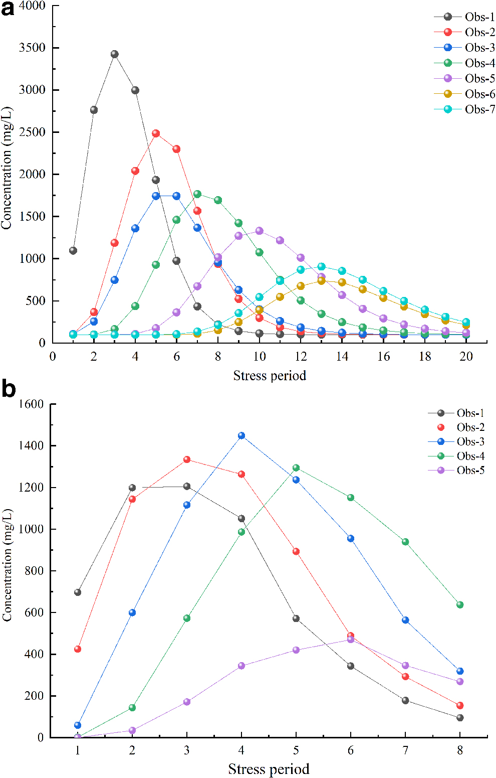
Unlike the actual problem, the hypothetical case contained no actual measured data. Therefore, it was necessary to forward run the pollutant transport simulation model of the cases (input the aquifer parameters and real information of pollution sources into the model) and obtain the pollutant concentration data for the observation wells in each stress period after operation as the measured data for identification. The simulated concentration data were disturbed by artificial noise to simulate the situation where the concentration measurements contained noise (the value of noise intensity is 0.05). Refer to the study of Mahar and Datta (1997; 2000) for the specific method of adding noise in simulated concentration. Figures 3 and 4 show the contaminant plume distributions and obtained pollutant concentration values, respectively.

FIG. 3.

(a) Contaminant plume distributions for case 1. (b) Contaminant plume distributions for case 2.

FIG. 4.

(a) Measured values in the observation wells in each stress period for case 1. (b) Measured values in the observation wells in each stress period for case 2.

Kriging surrogate model of the simulation model

During the iterative calculation process conducted to solve the GPSI problem with the 0–1MINLP, it was necessary to call the simulation model hundreds of times, thereby leading to a high computational load and long calculation period. This problem was solved effectively by establishing a surrogate model of the simulation model and linking the surrogate model as an equality constraint to the 0–1MINLP.

A surrogate model of the simulation model was established using the kriging method. The hydraulic conductivity and release intensities for the pollution sources in each release period were used as the input variables to establish the surrogate model and the concentration data for the observation wells were used as the output variables in the surrogate model. First, the Latin hypercube method was used to sample the hydraulic conductivity (the probability distribution of the hydraulic conductivity are shown in Tables 5 and 6) and release intensities for the pollution sources in their feasible regions. In total, 200 groups were sampled. Then, the sampled data were input to the simulation model, and the corresponding output concentration data for the 200 groups were obtained by running the simulation model. One hundred sixty groups of input and output data sets were prepared to train the surrogate model. According to the kriging method, the training code for the kriging surrogate model was written using MATLAB, and then the surrogate model was established by using kriging method.

Table 5.

Probability Distribution and Value Ranges of Hydraulic Conductivity for Case 1

Parameter partitions	Probability distributions	Mean	Ranges
I	Lognormal distribution	32.5	(30, 35)
II	Lognormal distribution	7.5	(5, 10)
III	Lognormal distribution	17.5	(15, 20)
IV	Lognormal distribution	27.5	(25, 30)
V	Lognormal distribution	42.5	(45, 50)

Table 6.

Probability Distribution and Value Ranges of Hydraulic Conductivity for Case 2

Parameter partitions	Probability distributions	Mean	Ranges
I	Lognormal distribution	32.5	(30, 35)
II	Lognormal distribution	27.5	(25, 30)
III	Lognormal distribution	17.5	(15, 20)

After obtaining the trained surrogate model, it is necessary to test the approximation degree of the surrogate model output to the simulation model output. Forty input and output data sets were used to test the accuracy of the surrogate model. The following two indicators were used to test the accuracy of the surrogate model.

The mean relative error (MRE) was calculated as follows. $M R E = \frac{1}{n} \sum_{i = 1}^{n} \frac{|y_{i} - ŷ_{i}|}{y_{i}} \times 100 % .$ (15)

The coefficient of determination (R²) was calculated as follows. $R^{2} = 1 - \frac{\sum_{i = 1}^{n} {(y_{i} - ŷ_{i})}^{2}}{\sum_{i = 1}^{n} {(y_{i} - ȳ_{i})}^{2}} .$ (16)

In these formulae, y_i is the output value of the ith sample in the pollution transport simulation model, $ŷ_{i}$ is the output value of the ith sample in the surrogate model, and $ȳ$ is the average of the output values for n samples in the pollution transport simulation model. Smaller values for MRE and R² values closer to 1 indicated that the surrogate model obtained higher precision at simulating the output of the simulation model, and thus the surrogate model could be used instead of the simulation model.

Optimization model

After establishing the surrogate model of the simulation model, an optimization model was established for identifying the hydraulic conductivity and characteristics of the groundwater pollution sources by comprehensively applying various mathematical methods, numerical simulation models (using surrogate models instead of simulation models), and limited data measurements to identify groundwater pollution source characteristics.

The sum of squared error between the monitored concentrations in the observation wells and the simulated calculated concentrations in the observation wells were minimized as the objective function. The location (regard as 0–1 integer variable), the hydraulic conductivity and release intensity of the pollution sources (regard as continuous variables) were used as the decision variables in the optimization model. The surrogate model for the simulation model was used as the pollution transport law constraint. A 0–1MINLP was established for identifying the hydraulic conductivity and information of pollution sources: $\begin{matrix} min z (β, K, Q) = \sum_{t = t_{0}}^{T} \sum_{k = k_{0}}^{N} {(C_{k}^{t} (t) - C_{k}^{t} (0))}^{2} \\ \{\begin{matrix} \begin{matrix} β_{i} = \{\begin{matrix} 1 \\ 0 \end{matrix} i = 1, 2, \dots n \\ \sum_{i} β_{i} = M \end{matrix} \\ K_{min} \leq K \leq K_{max} \\ Q_{min} \leq Q \leq Q_{max} \\ C_{k}^{t} (t) = f (K, Q) \end{matrix} \end{matrix} .$ (17)

where $β_{i}$ is the location of pollution sources, 1 represents the current location that is the real pollution source location, 0 represents the current location that is not the real pollution source location, Mis total number of real pollution sources, Kis hydraulic conductivity of each zone, Q is the release intensity of the contaminant sources during each release period, N is the number of observation wells, T is the total number of periods, $C_{k}^{t} (t) = f (β, K, Q)$ is the surrogate model of simulation model used to simulate the contaminant concentration, $C_{k}^{t} (t)$ is the simulated concentration of the contaminant at the observation point, and $C_{k}^{t} (0)$ is the measured value of the contaminant concentration at the observation point.

The ill-posedness of the two inverse problems in this study were evaluated by refering to Carrera and Neuman (1986), Draper and Smith (1998), Carrera et al. (2005) and Tarantola (2005), and it was found that the ill-posedness of the two GPSI inverse problems were weak and had little effect on solving the optimization model to obtain the optimal identification results.

Hybrid mixed HGA

The GA is a heuristic search method. However, there is some issues that GA is easy to lead premature convergence and into the plight of local optimum (Li and Tong, 1999; An et al., 2009; Guo and Zhou, 2009). The combination of homotopy algorithm and GA can avoid this shortcoming to a certain extent. The homotopy algorithm constructs a series of homotopy equations using known solution equations and equations to be solved, and then applies the GA to solve the homotopy equations step by step, so as to achieve the goal of “tracking” the solution of the equation to be solved from the known solution equation; therefore avoiding the drawbacks of the heuristic algorithm into local convergence to a certain extent (Abbasbandy et al., 2007; He and Li, 2013). The homotopy algorithm was combined with the GA to improve the disadvantages of its dependence on the initial population selection and preventing it from becoming trapped by a local optimum (premature convergence).

The principle of the combined use of homotopy method and GA is as follows: (1)

Based on the simulation model, an optimization problem $F (X)$ with a known solution was established. The specific method is to randomly give a set of hydraulic conductivity and information of pollution sources, then input them to the simulation model, and obtain the measured value of the contaminant concentration. The optimization problem $G (X)$ to be solved is the hydraulic conductivity and pollution sources identification problem of this study.

(2)

Determine the variation form of homotopy parameter $λ$ . Using homotopy algorithm to construct a cluster of homotopy equations based on $F (X)$ and $G (X)$ . The constructed homotopy equations are transformed into optimization problems.

The principle of constructing the homotopy equation is as follows: $\{\begin{matrix} H (X, λ) = λ \cdot G (X) + (1 - λ) \cdot F (X) λ \in [0, 1] \\ F (X) = f (x) - C_{0} \\ G (X) = f (x) - C_{o b s} \end{matrix} .$ (18)

where X is the hydraulic conductivity and information of pollution sources, $λ$ is the homotopy parameter, $f (x)$ is the surrogate model, C₀ is the calculated contaminant concentration obtained in the observation wells by substituting the assumed groundwater pollution source characteristics into the surrogate model, $C_{o b s}$ is the actual measured contaminant concentration in the observation well.

(3)

Take the solution of the optimization problem corresponding to $λ = 0$ as the initial solution of the homotopy optimization problem corresponding to $λ = 0.1$ , and apply GA to solve the optimization problem. Then take the solution of the optimization problem corresponding to $λ = 0.1$ as the initial solution of the homotopy optimization problem corresponding to $λ = 0.2$ . Perform the same procedure until the homotopy optimization problem $F (X)$ transformed into $G (X)$ , that is, the optimization problem corresponding to $λ = 1.0$ .

The path tracking process evolved gradually in the solution process, so the solutions of two optimization problems located adjacent to each other were also very close. Applying the solution of the (i-1)-th optimization problem as the initial solution for the i-th optimization problem ensured that the optimization process evolved gradually, thereby avoiding the premature convergence problem caused by selecting an inappropriate initial population.

By performing the above operations, we can start from the optimization problem with the known solution, and finally obtain the hydraulic conductivity and pollution source information to be identified through path tracking.

Results and Discussion

Accuracy of the surrogate model

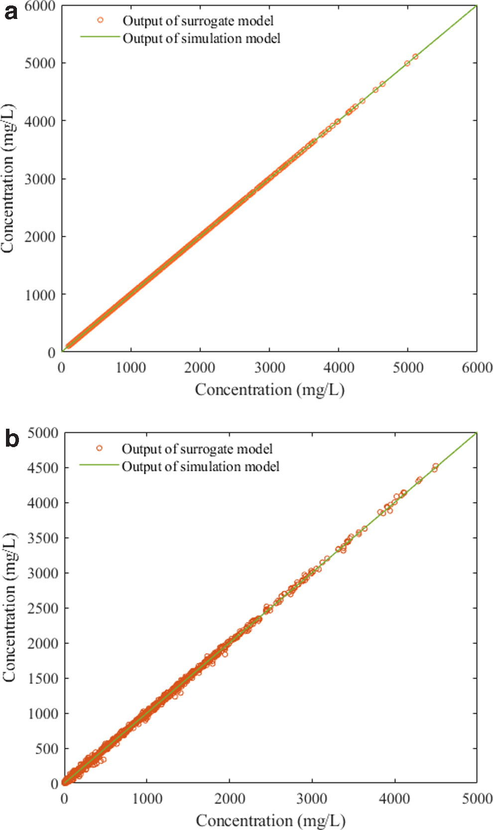
Forty sets of concentration data were obtained by entering 40 sets of hydraulic conductivity and release intensity data into the surrogate model. The fitting diagram for output concentrations of the surrogate model and simulation model are shown in Fig. 5. The accuracy evaluation indexes comprising R² and MRE for the surrogate model are shown in Tables 7 and 8.

FIG. 5.

(a) Contaminant concentration fitting diagram of surrogate model for case 1. (b) Contaminant concentration fitting diagram of surrogate model for case 2.

Table 7.

Accuracy of the Surrogate Model for Case 1

Observation well	R²	MRE
1	0.9999	0.42%
2	0.9999	0.67%
3	0.9998	1.00%
4	0.9999	0.76%
5	0.9999	0.60%
6	0.9997	0.67%
7	0.9996	1.08%

MRE, mean relative error.

Table 8.

Accuracy of the Surrogate Model for Case 2

Observation well	R²	MRE
1	0.9994	4.02%
2	0.9989	2.54%
3	0.9988	1.94%
4	0.9983	3.15%
5	0.9976	8.39%

Figure 5 clearly shows that the outputs from the surrogate model were very close to the outputs from the simulation model. Tables 7 and 8 show that the MRE values for the observation wells of case 1 were less than 1.5% and the MRE values for the observation wells of case 2 were less than 8.5%. The surrogate model approximated the simulation model very well and the accuracy was also satisfactory. Moreover, the R² were close to 1, thereby indicating that the accuracy of the surrogate model was very high. Thus, the surrogate model could be applied instead of the simulation model to linked to the 0–1MINLP.

Pollution source identification analysis results

The HGA was used to solve the 0–1MINLP. The homotopy equation was constructed by using the optimization problem for the known solution and the optimization problem for the unknown solution. The homotopy equations obtained by the transformation were transformed into the corresponding optimization problems and the optimization models for each optimization problem were established in turn, before applying the GA to solve each optimization model. The GA toolbox in MATLAB was used to solve the optimization model for each homotopy equation corresponding to the optimization problem. The main parameters of the GA were set as shown in Table 9, the meaning and settings of all the parameters in Table 9 can be found in the optimization toolbox of the MATLAB software.

Table 9.

Parameter Settings for the Genetic Algorithm

Parameter	Setting
Population size	20
Scaling function	Rank
Selection function	Stochastic uniform
Mutation function	Constraint dependent
Crossover function	Scattered
Direction	Forward
Generations	800
Other parameter settings	Default

The path was tracked from the known solution, so the initial population selection of each optimization model was appropriate, thus, the disadvantage that GA is easy to fall into premature convergence is avoided.

The identification results obtained using the HGA are shown in Tables 10 and 11. As the homotopy parameter $λ$ changed from 0 to 1, the optimization problem gradually changed from the optimization problem with known solution to the optimization problem to be solved. At the same time, the identified results gradually approached the true value of location, hydraulic conductivity, and release intensity. When $λ = 1$ , the location, hydraulic conductivity, and release intensity of the two cases were identified finally.

Table 10.

Results Obtained Using the Homotopy-Genetic Algorithm for Case 1

Homotopy parameter	Location		Hydraulic conductivity (m/d)					Release intensity (1 × 10⁵ mg/d)—S1				Release intensity (1 × 10⁵ mg/d)—S2
Homotopy parameter	S1	S2	I	II	III	IV	V	SP1	SP2	SP3	SP4	SP1	SP2	SP3	SP4
λ = 0	1	1	32.5	7.5	17.5	27.5	47.5	20	20	20	20	20	20	20	20
λ = 0.1	1	1	32.82	7.65	17.43	26.82	47.78	26.64	22.24	23.01	19.53	23.33	22.04	22.77	20.09
λ = 0.2	1	1	32.44	7.86	17.50	26.60	47.54	32.42	24.67	25.56	19.69	26.59	24.60	26.10	19.56
λ = 0.3	1	1	32.02	8.06	17.57	26.69	47.00	37.87	27.77	27.70	19.79	29.97	27.27	28.44	19.70
λ = 0.4	1	1	32.25	8.19	17.56	26.74	46.10	43.56	31.65	29.48	19.75	33.51	29.62	29.73	20.58
λ = 0.5	1	1	32.97	8.21	17.48	26.35	46.13	51.90	32.65	32.41	19.66	36.83	29.96	32.99	21.17
λ = 0.6	1	1	33.02	8.37	17.43	26.24	45.88	54.36	39.58	32.82	20.01	40.34	35.23	32.80	22.02
λ = 0.7	1	1	32.69	8.56	17.47	26.37	45.31	57.63	43.72	35.47	19.93	43.78	39.59	35.32	20.98
λ = 0.8	1	1	31.92	8.67	17.57	26.46	46.00	63.26	47.51	36.98	20.64	47.05	42.00	37.33	21.21
λ = 0.9	1	1	32.07	8.59	17.56	26.08	46.98	74.05	46.76	40.19	20.86	50.00	41.27	40.91	21.77
λ = 1.0	1	1	32.16	8.69	17.56	26.11	46.07	77.67	52.45	41.14	21.16	53.48	45.51	41.44	22.47

Table 11.

Results Obtained Using the Homotopy-Genetic Algorithm for Case 2

Homotopy parameter	Location				Hydraulic conductivity (m/d)			Release intensity (1 × 10⁵ mg/d) – S3				Release intensity (1 × 10⁵ mg/d) – S4
Homotopy parameter	S1	S2	S2	S4	I	II	III	SP1	SP2	SP3	SP4	SP1	SP2	SP3	SP4
λ = 0	0	0	1	1	32.50	27.50	17.50	10	10	10	10	10	10	10	10
λ = 0.1	0	0	1	1	32.20	27.99	17.96	12.23	12.45	11.10	10.41	12.10	11.61	11.01	10.16
λ = 0.2	0	0	1	1	32.26	27.76	18.09	15.28	13.30	14.05	9.47	14.32	13.17	11.98	9.91
λ = 0.3	0	0	1	1	32.33	27.48	18.14	17.46	16.05	14.45	9.70	16.63	14.56	13.19	9.61
λ = 0.4	0	0	1	1	32.38	27.62	18.18	19.85	18.43	15.81	10.01	18.60	16.28	14.13	10.23
λ = 0.5	0	0	1	1	32.53	27.53	18.09	22.33	20.56	17.07	10.13	20.77	17.76	15.27	10.07
λ = 0.6	0	0	1	1	32.81	27.55	17.96	25.01	22.18	19.00	10.17	22.79	19.33	16.24	10.07
λ = 0.7	0	0	1	1	32.95	27.26	17.98	27.56	24.18	20.26	9.92	24.98	20.71	17.37	9.88
λ = 0.8	0	0	1	1	32.93	27.17	17.98	30.12	26.35	21.41	9.91	27.14	22.19	18.54	9.87
λ = 0.9	0	0	1	1	33.03	26.99	18.10	32.69	28.32	22.94	9.71	29.20	23.75	19.50	10.01
λ = 1.0	0	0	1	1	33.10	26.96	18.05	35.28	30.36	24.33	9.69	31.29	25.27	20.59	10.07

Comparison of HGA and GA

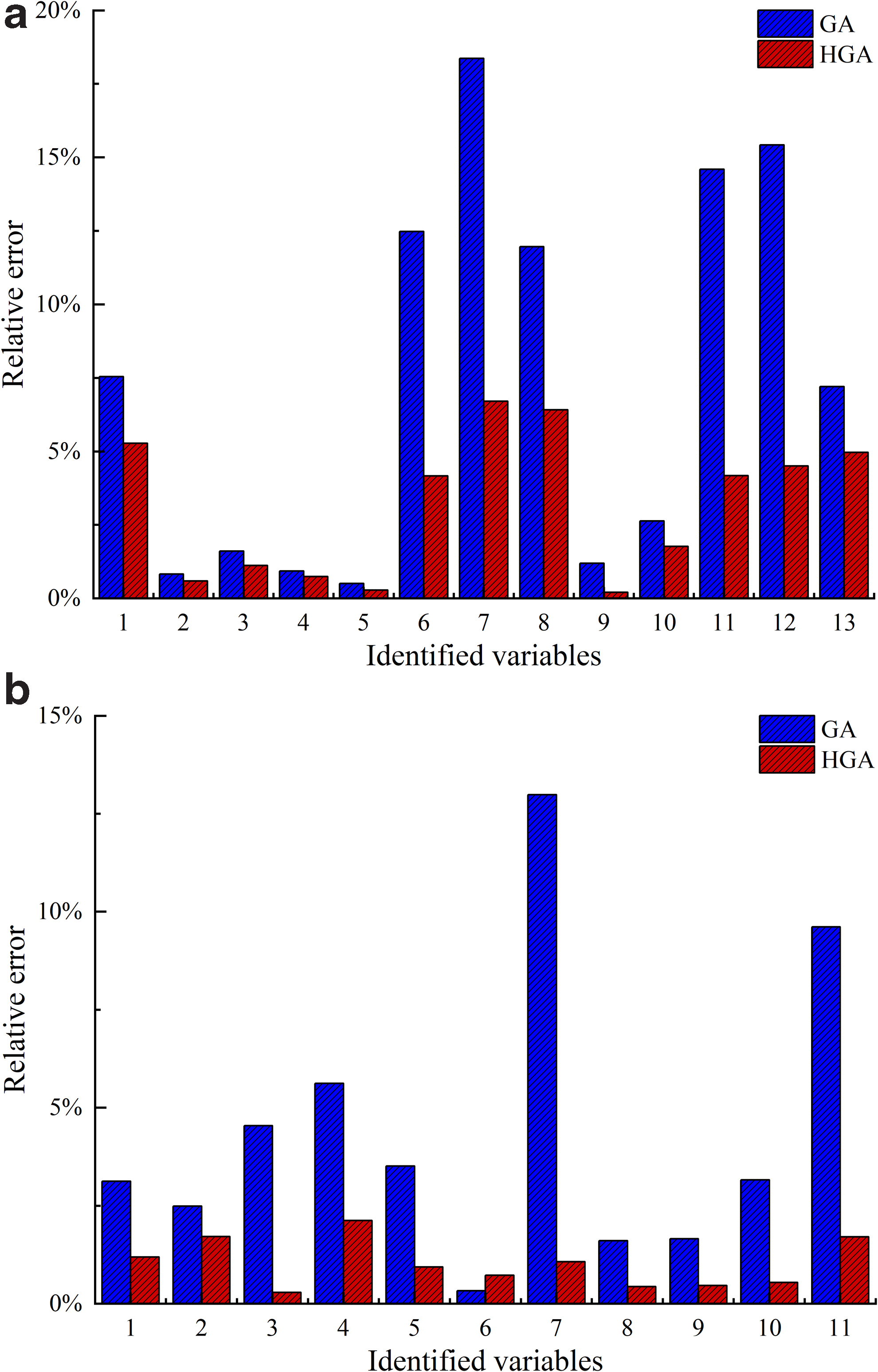
Tables 12 and 13 and Fig. 6 show that the identification results calculated using the HGA were closer to the true values of the pollution sources than those calculated using the GA alone. For case 1, when the GA was used to identify aquifer parameters and groundwater pollution source information, the maximum relative error of the identified results exceeded 17.5%, while the maximum relative error of the identified results obtained using the HGA did not exceed 7.5%. For case 2, the maximum relative errors of the identified results obtained by the HGA and GA exceed 12.5% and 2.5%, respectively. It can be seen from Fig. 6 that for any variable to be identified, the accuracy of the identified results obtained by the HGA is higher than that of the GA.

FIG. 6.

(a) Relative error histogram for case 1. (b) Relative error histogram for case 2.

Table 12.

Identification Results Obtained Using the Homotopy-Genetic Algorithm and Genetic Algorithm for Case 1

Method	Hydraulic conductivity (m/d)					Release intensity-S1 (1 × 105 mg/d)				Release intensity-S2 (1 × 105 mg/d)
Method	I	II	III	IV	V	SP1	SP2	SP3	SP4	SP1	SP2	SP3	SP4
GA	31.95	8.57	17.56	26.16	45.96	83.87	45.90	43.29	20.87	53.01	40.57	45.76	21.94
HGA	32.74	8.69	17.47	26.11	46.07	77.67	52.45	41.14	21.16	53.48	45.51	41.44	22.47
True value	34.56	8.64	17.28	25.92	46.2	74.56	56.22	38.66	21.12	54.44	47.5	39.65	23.64

GA, genetic algorithm; HGA, homotopy-genetic algorithm.

Table 13.

Identification Results Obtained Using the Homotopy-Genetic Algorithm and Genetic Algorithm for Case 2

Method	Hydraulic conductivity (m/d)			Release intensity-S3 (1 × 10⁵ mg/d)				Release intensity-S4 (1 × 10⁵ mg/d)
Method	I	II	III	SP1	SP2	SP3	SP4	SP1	SP2	SP3	SP4
GA	32.45	27.16	17.18	36.49	29.57	24.07	8.53	31.65	24.73	21.35	8.95
HGA	33.10	26.96	18.05	35.28	30.36	24.33	9.69	31.29	25.27	20.59	10.07
True value	33.5	26.5	18	34.55	30.65	24.15	9.8	31.15	25.15	20.7	9.9

This shows that the HGA is an efficient solution for a nonlinear optimization model because it can converge on a large scale and it does not depend on the initial population selected. The HGA has more advantages than the GA when solving the optimization model. The combination of homotopy algorithm and GA can improve the shortcoming of GA that is easy to converge prematurely.

Conclusions

After applying the proposed methods to GPSI, the following conclusions can be made. The combined application of homotopy algorithm and GA improves the shortcomings of GA that is easy to converge prematurely. The homotopy optimization problem is equivalent to a tracker, which evolves from the optimization problem with known solution to the optimization problem with unknown solution. Similarly, the solution evolves gradually as the homotopy optimization problem changes gradually. The solution to the previous homotopy optimization problem can be used as the initial population of the solution for the next homotopy optimization problem, and the solutions of two adjacent homotopy optimization problems are very close. In this way, an appropriate initial solution can be selected for the next homotopy optimization problem, thereby avoiding the problem caused by the dependence on the initial population and becoming trapped by local optimum for GA, so the solution obtained is closer to the true value. The identification results obtained by applying the GA and HGA separately were compared and analyzed. The identification results obtained by the HGA were closer to the true values of the pollution source characteristics, and thus the identified results were more effective.

The kriging surrogate model with high accuracy was linked to the 0–1MINLP instead of the simulation model. The kriging surrogate model could be directly called during the iterative calculations when solving the optimization while reduced a lot of calculation load as well as the time required. The 0–1MINLP based on a kriging surrogate model could simultaneously identify the hydraulic conductivity, location, and release history of pollution sources while maintaining a certain level of precision.

Footnotes

Acknowledgments

Special thanks are given to the journal editors and anonymous reviewers for their valuable comments and suggested revisions.

Author Disclosure Statement

No competing financial interests exist.

Funding Information

This study was supported by the National Nature Science Foundation of China (no. 41672232) and Jilin Province Science and Technology Development Project (no. 20170101066JC).

References

Abbasbandy

, Tan

, and Liao

S.J.

(2007). Newton-homotopy analysis method for nonlinear equations. Applied Mathematics and Computation. 188, 1794.

C.J.

, Jin

H.J.

, and Liu

C.H.

(2009). Improved Real-coding Genetic Algorithm. Networks Security, Wireless Communications and Trusted Computing, NSWCTC ‘09. Los Alamitos, USA: International Conference on IEEE, 2009.

Ayvaz

M.T.

(2010). A linked simulation-optimization model for solving the unknown groundwater pollution source identification problems. J. Contam. Hydrol. 117, 46.

Bagtzoglou

A.C.

, and Atmadja

(2005). Mathematical methods for hydrologic inversion: The case of pollution source identification. Water Pollution. 3, 65.

Bei

(2014). An Improved Ant Colony Algorithm Based on Distribution Estimation[C]//2014 Fifth International Conference on Intelligent Systems Design and Engineering Applications (ISDEA). New York, NY: IEEE, 2014.

Carrera

, Alcolea

, Medina

, Hidalgo

, and Slooten

L.J.

(2005). Inverse problem in hydrogeology. Hydrogeol. J. 13, 206.

Carrera

, and Neuman

S.P.

(1986). Estimation of aquifer parameters under transient and steady state conditions: I. Maximum likelihood method incorporating prior information. Water Resources Res., 22, 199.

Coetzee

, Coetzer

R.L.

, and Rawatlal

(2012). Response surface strategies in constructing statistical bubble flow models for the development of a novel bubble column simulation approach. Comput. Comput. Chem. Eng. 36, 22.

Draper

N.R.

, and Smith

(1998). Applied regression analysis. New York, NY: John Wiley & Sons.

10.

Garrigues

, and Ghaoui

L.E.

(2008). An Homotopy Algorithm for the Lasso with Online Observations. International Conference on Neural Information Processing Systems. Vancouver, British Columbia, Canada: Curran Associates, Inc..

11.

Gorelick

S.M.

, Evans

, and Remson

(1983). Identifying sources of groundwater pollution: An optimization approach. Water Resources Res. 19, 779.

12.

Guo

, and Zhou

(2009). An Algorithm for Mining Association Rules Based on Improved Genetic Algorithm and its Application. International Conference on Genetic & Evolutionary Computing IEEE. Los Alamitos, CA: IEEE.

13.

Guo

J.Y.

, Lu

W.X.

, Yang

Q.C.

, and Miao

T.S.

(2018). The application of 0–1 mixed integer nonlinear programming optimization model based on a surrogate model to identify the groundwater pollution source. J. Contam. Hydrol. 220, 18.

14.

X.Q.

, and Li

H.Y.

(2013). Based on the improved homotopy perturbation method for solving nonlinear equations. Appl. Mech. Mater. 275, 836.

15.

Hemker

, Fowler

K.R.

, Farthing

M.W.

, and von Stryk

(2008). A mixed-integer simulation-based optimization approach with surrogate functions in water resources management. Optimization Eng. 9, 341.

16.

Lapworth

D.J.

, Baran

, Stuart

M.E.

, and Ward

R.S.

(2012). Emerging organic contaminants in groundwater: A review of sources, fate and occurrence. Environ. Pollut. 163, 287.

17.

, and Tong

(1999). Partheno-genetic algorithm and analysis on its global convergence. Zidong. Xuebao Acta Auto. Sin. 25, 68.

18.

Mahar

P.S.

, and Datta

(1997). Optimal monitoring network and ground-water–pollution source identification. J. Water Resources Plann. Manage. 123, 199.

19.

Mahar

P.S.

, and Datta

(2000). Identification of pollution sources in transient groundwater systems. Water Resources Manage. 14, 209.

20.

Mahinthakumar

G.K.

, and Sayeed

(2005). Hybrid genetic algorithm—Local search methods for solving groundwater source identification inverse problems. J. Water Resource Plann. Manage. 131, 45.

21.

Mirghani

B.Y.

, Mahinthakumar

K.G.

, Tryby

M.E.

, and Ranjithan

R.S.

(2009). A parallel evolutionary strategy based simulation–optimization approach for solving groundwater source identification problems. Adv Water Resources. 32, 1373.

22.

Puangdownreong

, Kulworawanichpong

, and Sujitjorn

(2004). Finite convergence and performance evaluation of adaptive Tabu search. Knowledge-based intelligent information and engineering systems. Berlin, Heidelberg: Springer.

23.

Snodgrass

M.F.

, and Kitanidis

P.K.

(1997). A geostatistical approach to contaminant source identification. Water Resources Res. 33, 537.

24.

Sun

A.Y.

, Painter

S.L.

, and Wittmeyer

G.W.

(2006). A constrained robust least squares approach for contaminant release history identification. Water Res. Res. 42, 263.

25.

Singh

R.M.

, and Datta

(2007). Artificial neural network modeling for identification of unknown pollution sources in groundwater with partially missing concentration observation data. Water Res. Manage. 21, 557.

26.

Tamer Ayvaz

M.T.

(2016). A hybrid simulation–optimization approach for solving the areal groundwater pollution source identification problems. J. Hydrol. 538, 161.

27.

Tarantola

(2005). Inverse Problem Theory and Methods for Model Parameter Estimation. Philadelphia: Society for Industrial and Applied Mathematics, Philadelphia.

28.

Watson

L.T.

, and Wang

C.Y.

(1981). A homotopy method applied to elastica problems. Int. J. Solids Struct. 17, 29.

29.

Xing

Z.X.

, Qu

R.Z.

, Zhao

, Fu

, Ji

, and Lu

W.X.

(2019). Identifying the release history of a groundwater contaminant source based on an ensemble surrogate model. J. Hydrol. 572, 501.

30.

Y.D.

, Qian

L.F.

, and Chen

L.M.

(2007). Structural approximate analysis for composite barrel by using Kriging method. China Mech. Eng. 18, 988.

31.

Zwickl

D.J.

(2008). Genetic algorithm approaches for the phylogenetic analysis of large biological sequence datasets under the maximum likelihood criterion. Dissertations & Theses-Gradworks. 3, 257. Austin, TX: The University of Texas at Austin.