Modeling Coupled Reactive Transport Through Fault Zones: A Critical Review

Abstract

Fault zones significantly influence the migration of fluids in the subsurface and can be important controls on the local as well as regional hydrogeology. Hence, understanding the evolution of fault porosity/permeability is critical for many engineering applications (like geologic carbon sequestration, enhanced geothermal systems, groundwater remediation, etc.), as well as geological studies (like sediment diagenesis, seismic activities, hydrothermal ore deposition, etc.). The highly heterogeneous pore structure of fault zones along with the wide range of hydrogeochemical heterogeneity that a fault zone can cut through make conduit fault zones a dynamic reactive transport environment that can be highly complex to accurately model. In this article, we present a critical review of the possible ways of modeling reactive fluid flow through fault zones, particularly from the perspective of chemically driven “self-sealing” or “self-enhancing” of fault zones. Along with an in-depth review of the literature, we consider key issues related to different conceptual models (e.g., fault zone as a network of fractures or as a combination of damaged zone and fault core), modeling approaches (e.g., multiple continua, discrete fracture networks, pore-scale models), and kinetics of water/rock interactions. Inherent modeling aspects related to dimensionality (e.g., one-dimensional vs. two-dimensional) and the dimensionless Damköhler number are explored. Moreover, we use a case study of the Little Grand Wash Fault zone from central Utah as an example in the review. Finally, critical aspects of reactive transport modeling like multiscale approaches and chemomechanical coupling are also addressed in the context of fault zones.

Introduction

Faults can be defined as narrow structural discontinuities occurring in geologic formations, and can be comprised of a wide range of physical features like cracks, bends, folds, gouges, etc. The term “fault” can encompass a wide range of spatial scales from single fractures (∼mm to cm scale) to subsidiary faults and fracture networks (∼cm to m scale) to large-scale fault zones (∼km scale). In this discussion, the focus is predominantly on fault zones of at least >100 m scale. Depending on the scale of the fault architecture, they can be a highly complex and heterogeneous hydrogeological unit (Caine et al., 1996; Faulkner et al., 2010).

Faults play a critical role in many geological and engineered processes, like hydrocarbon migration (e.g., Sorkhabi and Tsuji, 2005; Rotevatn and Fossen, 2011), seismic activities (e.g., Raleigh et al., 1972; Aki, 1979), geothermal systems (e.g., Goyal and Kassoy, 1980; Moore and Simmons, 2013), hydrothermal ore formation (e.g., Garven et al., 1999; Wilkinson et al., 2009), groundwater flow and remediation (e.g., Bredehoeft, 1997; Iskandar and Koike, 2011), nuclear waste disposal (e.g., Bodvarsson et al., 1999; Orellana et al., 2019), and geological carbon sequestration (GCS) (e.g., Kampman et al., 2014; Patil, 2016). Faults commonly serve as important controls on local and regional fluid flow and migration, and can also be sources of critical seismic activities. Thus, faults are a very important focus of study among hydrogeologists, structural geologists, seismologists, and geoenvironmental engineers.

The importance of characterizing fault behavior to understand fluid migration was recognized early on by the petroleum exploration community (Fox, 1959; Jacobs and Kerr, 1965). Depending on the structure of the fault zone, it can either act as a conduit for hydrocarbon migration or serve as a seal for creating effective petroleum traps. Thus, faults can either turn out to be a boon (in case of effective fault traps) or a curse (in case of hydrocarbon leakage) for oil and gas exploration. Additionally, avoiding unintended migration of hydrocarbons into overlying groundwater aquifers through faults is an important part of the environmental management of the oil and gas industry.

Recognizing this fact, early studies were directed toward developing conceptual methods for effectively characterizing a fault as a conduit, a barrier, or a combined conduit/barrier system (e.g., Smith, 1966; Stanley, 1970). Later on, more in-depth understanding of the physical structure and the chemical and mechanical behavior of fault zones emerged through core and down-hole logging, interpretation and analyses of seismic and well data, outcrop studies, and laboratory testing (Knipe et al., 1998; Aydin, 2000), leading to predictive numerical modeling analyses (e.g., Moretti, 1998; Zhang et al., 2009). It could arguably be stated that the initial understanding of and the technical analysis framework for determining fault structure and fluid flow behavior have originated from the knowledge base of hydrocarbon exploration research.

Faults and fracture systems also play a very critical role in the functioning of an enhanced geothermal system (EGS). Geothermal energy is one of the most important renewable sources of cost-effective and environment-friendly power (Glassley, 2014). The efficient functioning and commercial viability of an EGS to serve as a source of power supply hinges on the effective and strategic management of the faults and fracture systems. Some EGS exploit the natural fractures in the geothermal reservoirs (e.g., Simmons et al., 2018), while others use hydraulic fracking to create new fracture permeability for fluid circulation (e.g., Moore et al., 2018). However, the extreme temperature differences resulting from the injection of “cold” fluid into a “hot” reservoir typically lead to rapid mineral precipitation in the fractures, which can plug the permeability of the circulation pathways.

One of the main challenges in EGS is to maintain sufficient fracture permeability (Patil and Simmons, 2020). Reaction kinetics of mineral precipitation/dissolution tend to be faster at higher temperatures, making fluid flow of geothermal fluids in faults a highly complex process. Several reactive transport modeling studies have attempted to characterize the coupled thermal-hydro-chemical (THC) processes (e.g., Kiryukhin et al., 2004; Xu et al., 2009). More recent developments include coupled thermal-hydro-chemical-mechanical (THMC) models (e.g., Sonnenthal et al., 2015; Salimzadeh and Nick, 2019; Yuan et al., 2020).

Faults are also an important consideration in designing geological disposal of anthropogenic waste. For example, in GCS, leakage of the injected CO₂ into unintended subsurface formations, like groundwater aquifers, or to the surface is considered a major environmental risk (Patil et al., 2017). Natural analogs of CO₂ leakage along faults have paved way for enhanced understanding of the reactive transport processes associated with the leakage of CO₂-enriched fluids (Shipton et al., 2005; Heath et al., 2009; Jung et al., 2014; Kampman et al., 2014). Few studies have focused on reactive transport modeling of CO₂ leakage along faults (Ahmad et al., 2015, 2016; Patil et al., 2017; Patil and McPherson, 2020). Additionally, CO₂-induced alterations in caprocks (especially in the fractures) are also an important issue for the integrity of a GCS system (Gherardi et al., 2007; Tian et al., 2014; Xiao et al., 2020).

Similarly, in nuclear waste disposal, it is important to understand and model the associated coupled reactive transport processes in fractured rocks to ensure environmentally safe deployment of the nuclear waste repository (e.g., Xu et al., 2003; MacQuarrie and Ulrich Mayer, 2005).

Faults are also a high-priority geologic feature to be considered in groundwater remediation and management. Often acting as high-velocity conduits for cross-formational fluid migration, faults may act as highways for contaminant transport into freshwater aquifers e.g., petroleum leaks (Flewelling et al., 2013), CO₂ leaks (Zheng et al., 2009; Siirila et al., 2012), heavy metal contamination (Lachhab et al., 2020), etc. Fault and fracture zones can also play a critical role in remediating existing contamination in groundwaters (e.g., Chambers et al., 2010; Mercer et al., 2010). Thus, understanding the reactive transport processes in fault zones is critical to almost all aspects of subsurface environmental engineering and management.

While it has always been understood that fluid flow in the subsurface is deeply coupled with the associated thermal, chemical, mechanical, and biological processes, numerical models often ignore one or more of these processes in the interest of computational simplicity, depending on how transient these processes are for the system being modeled. However, faults and fractured rocks are structures where the fluid flow is highly transient and the reactive transport scenario is dynamic. Thus, reactive transport modeling is all the more critical for fault-based fluid flow.

In this article, we present a critical review of modeling reactive transport through fault zones. In contrast to other reactive transport reviews, which focus on single fractures or fracture networks (e.g., Berkowitz, 2002; MacQuarrie and Ulrich Mayer, 2005; Deng and Spycher, 2019), we focus on the processes at the scale of fault zones, giving special emphasis to the “self-sealing” versus “self-enhancing” of the fault zone permeability owing to mineral reactions. In the following sections, we discuss conceptual models, continuum-based flow models, kinetics of geochemical reactions, Damköhler numbers, and special topics like chemo-mechanical coupling and multiscale reactive transport models. While modeling reactive transport through fault zones can be a highly complex topic requiring advanced modeling skills, our hope through this review is that the readers feel inspired to adopt some ideas presented in this study to create a meaningful analysis of their own.

Conceptual Models

The modeling approach chosen for a particular fault system depends on (1) the characteristic length scale (e.g., mm vs. km scale), (2) the aim of the modeling work (e.g., theoretical investigation of fundamental reactive processes vs. risk assessment for an engineered application), and (3) the level of detail in the available information (e.g., distributions of fracture geometry, density and connectivity, fault core thickness, composition and spatial distribution of phyllosilicates, etc.). Two broad categories of flow modeling approaches are prevalent in reactive transport studies, namely “pore-scale” models and “continuum-scale” or continuum models.

Pore-scale models are a popular choice to model fracture processes at the micrometer to millimeter scale, for example, mass transfer and reactions across the fracture aperture (Deng and Spycher, 2019). In the pore-scale approach, the fluid and rock interfaces are explicitly resolved with mesh discretization and the governing flow equations are based on the Navier–Stokes equations (Molins, 2015; Deng and Spycher, 2019). Such models are useful for understanding some of the fundamental reactive transport processes in the pore spaces, like surface reaction controls on the rate of mineral dissolution (e.g., Molins et al., 2014), the impact of surface roughness (e.g., Deng et al., 2018a), etc. Also, the pore-scale reactive transport processes are studied over much smaller time scales (typically over minutes). Given the smaller spatial and temporal scales of such processes, some of these processes can be experimentally verified in the laboratory, offering the advantage of direct verification of the numerical pore-scale model results (e.g., Molins et al., 2014).

In contrast, continuum-scale flow models assume a combined fluid and rock representation in each discretized mesh cell and the governing flow equations are based on Darcy's law. Based on the conceptual representation of the fault permeability, continuum-scale models are subcategorized into Discrete Fracture Network (DFN) models and Continuum models. DFN models represent the domain as a set of fracture, with properties of each fracture individually defined (Jing and Stephansson, 2007). In contrast, continuum models adopt some form of aggregation strategy to represent the fracture permeability in the model. The primary difference between DFN and continuum models stems from the concept of representative elementary volume (REV), which can be defined as the smallest spatial scale at which the properties of the domain can be assumed to be homogeneous. DFN models usually operate at the sub-REV scale, whereas continuum models operate at or above the REV scale (Berkowitz, 2002). However, since they both deal with flow using Darcy's law, they fall under the “continuum-scale” category.

While DFN models tend to be more accurate for flow and transport calculations through fractured media, they are limited by the spatial and temporal scale that they can be typically applied to (Deng and Spycher, 2019). At the scale of fault zones (from hundreds of meters to few kilometers), the resolution in the available data and characterization of the fracture networks is usually not enough for developing DFN models for that scale. Therefore, the most common choice for long-term modeling of reactive transport through fault zones are continuum models. As rules of thumb, (1) pore-scale or DFN models are applied when information related to fracture geometrical properties, density, and interconnectivity is available, and continuum models are applied when only the effective porosity/permeability of the fault can be estimated, and (2) model complexity decreases with increasing spatial and temporal scale. Figure 1 presents the scale dependency of the choice of modeling approach in a schematic.

FIG. 1.

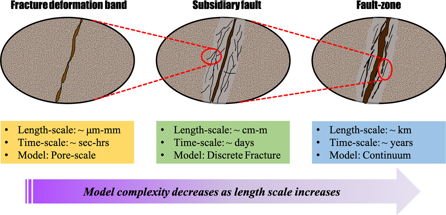
Schematic of the scale dependency of the flow modeling approach chosen for different fault types. Depending on the interest of the modeling exercise, fault processes can range in spatial scale from micrometers to kilometers and in time scale from seconds to thousands of years. Therefore, the spatiotemporal resolution in the data and models can vary tremendously. Model complexity will typically decrease with large spatiotemporal scale.

Continuum models can have either a single continuum or multiple continua (e.g., dual porosity, dual permeability, multiple interacting continua [MINC]). Single continuum models are the simplest in this category, wherein the entire fault zone is treated as an effective porous medium. The dual porosity approach was the first multiple continua approach that was developed early on to deal with fractured porous media (Warren and Root, 1963). This approach represents the fracture network in an idealized geometric pattern with different porosity values assigned for the fractures and the matrix (unfractured portion of the host rock). Fluid pressure and temperature interaction is considered between the matrix and fractures, but global flow is assumed only through the fractures (matrix is assumed to be relatively impermeable).

In concept, dual porosity models are similar to DFN models, which also assume flow through fractures only, and they both serve the same purpose (Lee et al., 1999). The main difference is that, unlike DFNs, dual porosity models do not simulate the actual fractures but rather approximate the aggregate flow through the fracture network through one of the continua representing the overall porosity of the fracture network. Several applications of the dual porosity approach are found in the literature (e.g., Gerke and Van Genuchten, 1993; Larsson and Jarvis, 1999; Delshad et al., 2002; Taron and Elsworth, 2009).

An important extension of the dual porosity model is the multiple interacting continua or “MINC” model (Narasimhan and Pruess, 1988). With this approach, several “hierarchies” of heterogeneity, or sets of parallel continua at a given hierarchy level, can be set depending on the data availability. This structure provides the ability to simulate the differences in the diffusivities in heterogeneity in a much refined and precise manner, and is useful to applications like geothermal systems (e.g., Xu and Pruess, 2004; Itoi et al., 2010) and contaminant transport in groundwater (Xu et al., 2001; Chen et al., 2015).

Both the dual porosity and the MINC approaches described above treat the transport through the fractures with advection and the matrix with diffusion. To treat global advective flow and transport through both the highly permeable and the low permeable materials, the dual-permeability approach can be used. With this approach, global flow is assumed through both the fractured continuum and the matrix.

To develop a conceptual model for fault zones, the “architecture” and permeability structure of a fault zone needs to be examined and understood. According to Caine et al. (1996), three regions within a fault zone have distinct fluid flow properties, namely the damaged zone, the fault core, and the protolith. Most of the displacement during faulting gets accommodated in the fault core. It is typically a region of low porosity and permeability. The damaged zone is a highly heterogeneous region that accommodates fractures, bends, and folds, and is typically a region of high porosity and permeability. The protolith is the unaltered reservoir rock surrounding the fault core and the damaged zone. The effective permeability and the flow behavior (e.g., conduit, barrier, mixed) of the fault can be roughly determined by the composition of these three fault elements.

Large regional scale fault zones are commonly composed of smaller faults and associated components. These smaller faults will have their own damaged zone within the damaged zone of the larger fault zone. However, common anatomical model of a central fault core (accommodating most of the displacement from faulting) enveloped by a highly heterogeneous damaged zone is typical in many studied fault zones (Fossen, 2020).

The effective permeability structure of the fault will be determined by individual behaviors of the damaged zone and fault core as barriers or conduits. Therefore, it is critical to characterize their permeabilities as meaningfully and accurately as possible.

The effective damaged zone permeability depends on the permeability of the host rock, composition of macroscale fractures, and low permeability deformation bands. In low-porosity host rock, the fault permeability is controlled by the density and connectivity of macrofractures. Moreover, even though the fractures and slip in the damaged zone may have significantly higher permeability as compared with the host rock, the effective permeability of the damaged zone is determined by the interconnectivity of the fracture network. Damaged zones are commonly characterized by measuring the density of fractures as a function of distance from the “central” fault core. Typically, this fracture density decreases exponentially with increasing distance from fault core (Faulkner et al., 2010).

The permeability of the fault core is typically a function of the host rock and the composition of gouges. Two distinct types of fault gouge are found in studies of natural faults. The first type is made of granular siliclastic material (predominantly quartz) and the second type consists of phyllosilicates (clay-rich shale material). The phyllosilicate gouge will typically have much less permeability. Sedimentary basin fault zones are typical of having sand shale gouges that serve as longitudinal (along the fault plane) conduits and lateral (across the fault plane) barriers (Faulkner et al., 2010).

An index, Fa, proposed by Caine et al. (1996) for characterizing the nature of fluid flow through a fault, can be useful in depicting the overall permeability of the fault zone. Fa is defined as: $\begin{matrix} F a & = \frac{d a m a g e d z o n e w i d t h}{t o t a l f a u l t w i d t h} \\ = \frac{d a m a g e d z o n e w i d t h}{d a m a g e d z o n e w i d t h + f a u l t c o r e w i d t h} \end{matrix}$ (1)

This index may be used to assess the sensitivity of flow and related processes to the permeability structure of the fault by keeping the fluid flow properties of the two regions consistent and merely varying the Fa values to evaluate and compare impacts of different effective structures (as demonstrated by Patil et al., 2017). Clearly, increasing Fa value will lead to increasingly conduit-type behavior, whereas decreasing Fa value will lead to increasingly barrier-type behavior.

Many kilometer scale faults in sedimentary basins can simultaneously serve as conduits for longitudinal and barriers for lateral fluid flow and reactive transport (Matthäi, 2003; Faulkner et al., 2010). Outcrop observations also show that the most common fault permeability structure is that of a conduit along the fault and a barrier across the fault (a conduit-barrier system) (Bense et al., 2013). Juxtapositioning of reservoirs and seal layers along the fault length (as a result of faulting) is another crucial aspect in determining the sealing potential of the fault and whether the fault acts as a barrier to lateral flow.

In comparison to undeformed formations, fault zones are typically a more dynamic reactive transport environment. The relatively drastic changes in fluid composition and temperatures can significantly affect the composition of faults. Reactive fluid transport along the fault can lead to mineralogical changes typically accompanied by a redistribution of local stress and a change in the rock mechanical properties (Deng and Spycher, 2019). This phenomenon can impact the mechanical strength of the fault, potentially affecting the character of fault slip in response to earthquakes in the deeper crust (Bense et al., 2013). Fully coupled reactive transport modeling of such processes is one of the most effective ways of attempting to characterize the highly evolving fault permeabilities.

Numerical Models

All continuum models develop their governing equations from the principle of mass (or energy) conservation. Most subsurface flow (especially at the scale of hundreds of meters to kilometers) is typically within the regime of Darcy's law (slow, viscous flow with Reynolds number [Re] <1). The governing multiphase flow and reactive solute transport equations, as described in the widely used TOUGHREACT software (Xu et al., 2012), are presented briefly below. For more detailed instructions on the mathematics and the implementation of such equations, the reader is encouraged to look into several related resources (e.g., Yeh and Tripathi, 1991; Steefel and Lasaga, 1994; Lichtner, 1996; Clement et al., 1998; Bacon et al., 2000; Xu, 2001; White and Oostrom, 2003; MacQuarrie and Ulrich Mayer, 2005; Xu et al., 2012).

The basis mass and heat conservation equations are of the general form: $V_{n} \frac{Δ M_{n}}{Δ t} = \sum_{m} A_{n m} F_{n m} + V_{n} q_{n}$ (2)

where subscript n is for a grid cell, subscript m is for all the connected grid cells, V_n is the integrated volume of the grid cell, M_n is the mass (or energy) accumulation in the grid cell, t is the time step, A_nm is the connected surface area between grid cell n and m, F_nm is the average mass (or energy) flux across A_nm, and q_n is the average source/sink term per unit volume.

The fluid flow is assumed to be following the Darcy's law, which is of the form: $μ_{β} = - k \frac{k_{r β}}{μ_{β}} (\nabla p_{β} - ρ_{β} g)$ (3)

where subscript ß represents the fluid phase index, u is the Darcy flux for the fluid phase, k is the absolute permeability, k_r is the relative permeability of the fluid phase, μ is the viscosity of the fluid phase, p is the fluid pressure of the phase, ρ is the fluid density of the phase, and g is the gravitational acceleration.

Flow in fault zones can sometimes be transient, wherein the local velocity values may fall beyond the Darcian regime (Re >1). In such cases, there is lesser volume of fluid pushed for the same amount of pressure drop (as compared with Darcian flow). Flow through fractures with higher than Darcian flow rates are commonly dealt with the Forchheimer equation (Lage, 1998; Bené, 2000), wherein an additional quadratic or cubic term is added to the Darcy's law equation [Eq. (3)] to account for the nonlinear relationship of flow rate and pressure drop. However, the mathematical derivation of the Forchheimer equation is not straightforward. There are several studies that attempt at calibrating the associated Forchheimer coefficient based on experimental data (e.g., Takhanov, 2011). Barree and Conway model (Barree and Conway, 2004) is another similar approach to model non-Darcian flow through fractures, which is known to provide better fit to the experimentally derived nonlinear relationship compared with the Forchheimer model (Zhang et al., 2019).

The accurate estimation of these fitted coefficient values can be challenging in multiphase flow systems and reactive environments, and may need extensive experimental data sets (both field and laboratory) to calibrate these models. Such non-Darcian behavior may be more relevant for near-injection flow through fractures, as in the case of geothermal systems or artificial recharging of fractured aquifers (e.g., Mwetulundila and Atangana, 2020). Even though the rest of discussion will assume to Darcian flow, the reactive transport concepts can be adapted to Forchheimer-based models (e.g., Khoei et al., 2020).

Multicomponent chemical solute transport in the aqueous phase is defined based on the advection-diffusion equation in the form: $\frac{Δ t}{V_{n}} \sum_{m} A_{n m} [u_{n m} C_{n m}^{j} + D_{n m} \frac{C_{m}^{j} - C_{n}^{j}}{d_{n m}}] = Δ m_{n}^{j} - q_{n} Δ t - R_{n} Δ t$ (4)

where j is the subscript marking a particular chemical component, C is the molar concentration of the component, D is the effective diffusion coefficient, d is the nodal distance between the grid cells, and R is the cumulative geochemical reaction source/sink term.

While certain minerals can be considered at equilibrium with fluid, the dynamic multimineral reaction scenario typical for a fault zone calls for treating most water/rock interactions kinetically. The rates of mineral reactions are calculated using a rate law derived from transition state theory by Lasaga et al. (1994), which is of the form:

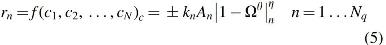
where n subscript is for a mineral, r_n is the dissolution/precipitation rate of the mineral n in moles per kg H₂O and unit time, k_n is the temperature-dependent rate constant or specific rate in moles per unit mineral surface area and unit time, A_n is the specific reactive surface area per kg H₂O, Ω_n is the mineral saturation ratio, and θ and η are empirically derived parameters. r_n has a positive value for precipitation and a negative value for dissolution.

The general form of the multimechanism, temperature-dependent rate constant is given as: $\begin{matrix} k & = k_{25} exp [- \frac{E}{R} (\frac{1}{T} - \frac{1}{298.15})] \\ + \sum_{i} {k_{25}}^{i} exp [- \frac{E^{i}}{R} (\frac{1}{T} - \frac{1}{298.15})] \prod_{j} {a_{i j}}^{n_{i j}} \end{matrix}$ (6)

where subscript or superscript i is the additional mechanism index and j is the index of the species involved in the mechanism, for example, H+ for acid mechanism (Xu et al., 2006). The rate constant value calculated by Equation (6) gets fed into the rate equation given in Equation (5). Palandri and Kharaka (2004) developed a compilation of the experimentally derived values for the above rate parameters from existing literature.

To simulate fully coupled reactive transport flow through fault zones, the feedback of mineral dissolution/precipitation reactions on the value of porosity ϕ can be calculated simply from the changes in the volume fractions of the minerals as: $ϕ = 1 - \sum_{m - 1}^{n m} f r_{m}$ (7)

where nm is the number of minerals and f_rm is the volume fraction of mineral m.

Permeability changes associated with the porosity fluctuations calculated in Equation (7) can be calculated (with certain simplifying assumptions) using the cubic law relationship for fractures (Steefel and Lasaga, 1994) and the Kozeny-Carman relationship for matrix (Berryman and Blair, 1987; Costa, 2006). Permeability modification using a cubic law relationship can be estimated as: $k = k_{i} {(\frac{ϕ}{ϕ_{i}})}^{3}$ (8)

where k_i and ϕ_i are the initial permeability and porosity. Permeability modification using a Kozeny-Carman relationship can be estimated as: $k = k_{i} \frac{{(1 - ϕ_{i})}^{2}}{{(1 - ϕ)}^{2}} {(\frac{ϕ}{ϕ_{i}})}^{3}$ (9)

The relationships presented in Equations (8) and (9) are idealized with simplifying assumptions. In reality, permeability modification in the subsurface is a highly complex subject that is yet not fully understood. Laboratory and field evidences have shown that even relatively small quantity of mineral precipitations can cause a large drop in the fracture permeability if the precipitates plug the fracture aperture. This can be especially true in the case of clay formation in the fault zones. The above relations are useful for a generic first-hand analysis when minimum details about the fault zone are available and should be modified based on site-specific needs. The reader is encouraged to look into the substantial literature available on the topic of permeability modification for further instructions (e.g., Chilingar, 1964; Nelson, 1994; Crawford et al., 2002; Ehrenberg and Nadeau, 2005; Yang and Aplin, 2010).

Example of Reactive Transport Modeling of Fault Zones

In this study, a multiphase reactive transport model of leakage of CO₂ and CO₂-enriched water along a real fault zone in central Utah is presented as an example for the readers. This model was developed and analyzed in detail by Patil et al. (2017).

Reservoirs of naturally occurring CO₂ provide an excellent opportunity to understand the long-term impact of sequestering anthropogenic CO₂ in subsurface formations (Evans et al., 2004; Allis et al., 2005). The Little Grand Wash Fault zone (LGWF) near Green River, Utah, is a leaking fault system that cuts into a deep reservoir of naturally occurring CO₂. CO₂-enriched fluids migrate along the conduit fault zone all the way to the surface, evidenced by calcite/aragonite cement in fractures and massive travertine (freshwater limestone) deposition at the surface along the fault line (Fig. 2a, b) (Burnside et al., 2013). Thus, the LGWF displays self-sealing behavior by calcium carbonate (CaCO₃) precipitation in the fault outcrops.

FIG. 2.

(a) Travertine precipitation along the fault trace, (b) subsurface fractures in the fault zone filled with CaCO₃ (after Patil et al., 2017), and (c) schematic of the conceptual flow model of the LGWF (after Vrolijk et al., 2005). CaCO₃, calcium carbonate; LGWF, Little Grand Wash Fault zone.

The LGWF may act as a barrier to lateral flow, especially due to juxtaposing of formations as a result of faulting (Dockrill and Shipton, 2010). The different formation waters flowing in from the San Rafael Swell in the NE-SW direction become stagnant in the footwall of the fault. CO₂ originating from deeper formations migrates up along the fault and mixes with these waters. The inferred potentiometric surface of the Navajo Sandstone from the recharge area to the leakage location suggests that artesian pressures exist below the fault location (Hood and Patterson, 1984), driving CO₂-enriched waters from the Navajo-Wingate and Entrada formations to the surface along the LGWF. Crystal Geyser is a cold-water geyser along the LGWF, which erupts CO₂-enriched groundwater from the Navajo-Wingate aquifers, and is a site of active (present-day) travertine deposition (Shipton et al., 2005; Heath et al., 2009). Figure 2c provides a schematic overview of the LGWF hydrogeology (Vrolijk et al., 2005).

The fault depth of top 300 m was modeled as a one-dimensional (1D) dual-permeability domain, with the fault core and damaged zone simulated as separate domains of the fault with different porosity and permeability values. Vertically upward migration and multiphase reactive transport along this fault domain was simulated using the TOUGHREACT simulator (Xu et al., 2006) for 1,000 years. The mineralogy and inlet boundary fluid composition were constrained based on the actual hydrogeochemical conditions at the LGWF location. Detailed model description and parameter values are documented in Patil et al. (2017).

A numerical index was developed to quantify the “rate of self-sealing” of the fault using the changes in the porosity of the damaged zone and the fault core. The porosity of the fault was calculated by taking the weighted average of the damaged zone and fault core porosity based on the widths of the damaged zone and fault core. The rate of fault self-sealing was calculated as: $F s = \frac{[\frac{(ϕ_{0} - ϕ)}{ϕ}] * 100}{t}$ (10)

where ϕ₀ is the initial porosity of the fault, ϕ is the porosity of the fault after t years of simulation time, and Fs is the rate of fault self-sealing in percentage change in porosity per year. Positive value of Fs indicates a self-sealing behavior, whereas negative value indicates a self-enhancing behavior. Fs was then calculated spatiotemporally to show the evolution of Fs throughout the simulation.

Two key water-rock reaction sequences were evident from the modeling, namely the dissolution of primary carbonates followed by precipitation of secondary carbonates, and the incongruent dissolution of feldspars followed by precipitation of secondary clays. The porosity in the damaged zone increased in the bottom half of the fault depth (∼150 to 300 m), and decreased in the top half (∼0 to 150 m). Starting with a damaged zone porosity of 0.4, the value increased up to 0.44 (10% increase) in the bottom half and decreased to as low as 6% (450% decrease) in the top few meters of fault depth over the simulation time of 1,000 years. Calcite precipitation was the single largest contributor to porosity reduction in damaged zone, followed by dolomite and gypsum. This result is in agreement with field observations (Fig. 2) and outcrop analyses (Burnside, 2010; Dockrill and Shipton, 2010) of the LGWF. Figure 3 presents key results of the LGWF model.

FIG. 3.

Key results of the LGWF model from Patil et al. (2017). Evolution of (a) gas saturation, (b) pH, (c) porosity, and (d) calcite abundance in the damaged zone, and (e) porosity and (f) fault sealing rate Fs for the overall fault (after Patil et al., 2017).

The results from the above model also demonstrate a system that is simultaneous “self-sealing” (permeability reduction) and “self-enhancing” (permeability enhancement). The facts that minerals dissolving at depth precipitate near the surface and that there is a “dissolution front” that keeps shifting upward along time, evidence that permeability modification due to reactive transport along a fault zone can be a highly spatiotemporally varying problem for which reactive transport modeling becomes an important piece of the puzzle (alongside outcrop analysis, downhole measurements and laboratory testing).

Usually, mineral precipitation along a fault zone can be either caused by changes in fluid pressure/temperature (e.g., Herman and Lorah, 1987; Han et al., 2013; Yehya and Rice, 2020) or by mixing of fluids with different compositions (e.g., Goldhaber et al., 1983; May, 2005) leading to supersaturation of a solid mineral phase. Many fault systems, with vertically upward transport along the fault plane and lateral mixing with fluids in the protolith or the adjacent host rocks, may have both the mechanisms at play. Such systems may require a two-dimensional spatial representation with predominantly advective transport along the fault plane and diffusive transport across the fracture walls into the matrix.

At the LGWF system, while the fluids flowing up along the fault do interact with the reservoir fluids in the footwall of the fault zone (as evidenced by Kampman et al., 2014; Busch et al., 2014), it was found by Patil et al. (2017) through geochemical modeling that the rapid pressure loss mechanism precipitated mineral mass about two to three orders of magnitude greater than the lateral mixing mechanism. Hence, it was justified to adopt a 1D simplification of the model.

The choice of multiphase flow parameters (relative permeability and capillary pressure [RP-CP]) can also make a significant impact on the reactive transport predictions. For comparison, Patil et al. (2017) demonstrated the impact of employing six distinct RP-CP formulations and parameter sets on the predictions on the LGWF model. Results showed that the relative permeability parameters had the most pronounced impact on the depth of dissolution front and the amount of calcite precipitation along time. In complex multiphase multimineral systems like the LGWF, applying “standard” relative parameters obtained from the literature may not yield accurate results, and appropriate measures should be taken to ensure that the data applied to the models are closely relevant to the actual system. Laboratory data, whenever available, should be given priority.

Kinetics of Water-Rock Interactions

So far, in this review, one half of the reactive transport problem, which is the fluid flow, has been discussed. In this section, the other half, which is the geochemical reactions and their kinetics will be discussed. Since the interest of this review has been permeability modification in fault zones owing to reactive transport, we will focus this discussion on the kinetics of water-rock reactions.

Water-rock reactions are heterogeneous surface reactions and most surface reactions have a sequential process that involves the following steps (Fogler, 1992; Lasaga, 1998; Levenspiel, 1999): (1)

Mass transfer of the reactant aqueous species to the near vicinity of the solid surface.

(2)

Adsorption of the reactant species onto the mineral surface.

(3)

Surface reaction between the mineral and the aqueous species.

(4)

Desorption of the product species from the mineral surface into the fluid.

(5)

Mass transfer of the product species from the near vicinity of the surface into the bulk fluid.

Steps 1 and 5 usually happen through diffusion (Lasaga, 1984). Some reaction models combine steps 2, 3, and 4 as surface reaction.

Each step in the heterogeneous reaction model offers resistance to the reaction (an energy barrier to cross). In sequential mechanisms, the slowest of the steps, offering the most resistance, turns out to be the “rate-determining” or “rate-limiting” step. This is because in a sequence, the slowest reaction becomes a bottleneck for the overall rate. Hence, if the transport of species to or away from the solid surface is much slower than the surface reaction rate (including adsorption/desorption), then the overall reaction rate is “transport controlled.” If the opposite is true, the overall reaction rate is “surface reaction controlled.” Some reactions can have mixed rate controls, when the mass transport rates are comparable to the surface reaction rates (Berner, 1978).

Most mineral dissolution reactions at low temperatures are surface controlled, that is, the surface reaction rates of mineral dissolution are very slow compared with the diffusion rates in the fluid. However, some exceptions to this observation could be dissolution reactions happening at very low pH conditions, wherein the reaction rates are faster. For example, calcite dissolution is diffusion controlled at pH <3 and 25°C (Berner and Morse, 1974). Also, many reactions at high temperatures tend to be fast enough for the reaction to be either diffusion controlled or mixed.

Evaluation of these individual rate controls shows that the relative significance of diffusion versus surface reaction may be affected by factors like the ratio of the reactive surface area to the diffusion cross-section, the porosity of the medium, and the tortuosity of the flow path. It also depends on the degree of disequilibrium and varies with the reaction progress (Murphy et al., 1989).

The reason why it is so important to know about the rate control over a reaction is because that determines how we would define the rate law for that particular reaction. If a reaction has mixed control, then both (1) the rate of diffusion of species to and away from the interface to the bulk flow, as well as (2) the rate of attachment or detachment of species from active sites on the mineral surface, should be included in the rate law. For a multicomponent system, this becomes very complex and computationally expensive to calculate, especially in reactive transport modeling (Steefel and Lasaga, 1994). Rate laws applied in most standard reactive transport will assume surface-controlled water-rock reactions.

The rate constant k in the kinetic rate law [Eq. (5)] is one of the two important parameters on which the reaction rate depends. The two most significant factors dictating the value of k are pH and temperature. In general, dissolution reaction rates increase with decrease in the pH of the solution. Mathematically, k ∝ (a_H)ⁿ where a_H is the activity of proton. n is determined experimentally and can be noninteger value, which is explained by the varied surface energetics (Lasaga, 1984). For some minerals like aluminosilicates, the value of k reduces as the pH increases until slightly alkaline. As the solution becomes more alkaline, the value of k increases (Lasaga, 1984). Rates are generally the slowest when the solution has a near-neutral pH (Palandri and Kharaka, 2004).

The pH dependence of rate constant is accommodated in the general rate equation by including multiple reaction mechanisms. The most extensive data are available for acid and base mechanism, catalyzed by the H+ and OH− ions. The temperature dependence of k is defined by the Arrhenius law. The general mathematical form of the multimechanism, temperature-dependent rate constant is given in Equation (6).

Reactive mineral surface area, second of the two most important parameters in the rate law [Eq. (5)], is defined as the total active/reactive area of a mineral in m² per kg H₂O. It is a measure of (1) how much mineral surface is in contact with the fluid, and (2) how much of the surface area is active in reaction. The importance of reactive surface area in the rate control was realized early on (Lasaga, 1981; Helgeson et al., 1984). There have been several studies, which have developed methods and protocols to measure and estimate the effective reactive surface area, using microscopic imaging and other quantitative techniques (e.g., Rufe and Hochella, 1999; Landrot et al., 2012; Lai et al., 2015). Yet, the mathematical representation of the evolution of reactive surface area of minerals in natural environments remains to be a challenge, especially in large-scale continuum models.

There are two main reasons for this disparity. First, the effects of surface roughness and preferential flow paths (channeling) on the reactive area are very difficult to measure in situ. Even if the in situ reactive area is measured by techniques described by Lasaga (1995) and the proceeding literature, it will be very difficult to estimate the variance of the measured reactive area over the scale of the model due to lack of information about heterogeneity. Second, the reactive area evolves continuously along time as mineral precipitation/dissolution reactions change the mineral surface along the flow path.

Common methods to estimate surface area are by (1) geometric estimation using mineral grain size, and (2) BET surface area measurements. The grain structure of different minerals may result in different surface areas. For example, sheet silicates owing to their plate-like structure provide an order of magnitude greater surface area as compared with carbonates or feldspars. Swelling of clays is a phenomenon that can have huge impacts on the flow patterns and greatly alter reactive surface area. Extrapolating surface areas measured by these methods to field-scale use is a research area with large uncertainties.

The research community's understanding of the kinetics of water-rock interactions and its application to reactive transport modeling has made significant strides in the last couple of decades. Yet, precautions should be taken while adopting generic rate formulations for every mineral under consideration. While it is not practical to self-test the kinetics of each mineral of interest in the laboratory, it is advisable to conduct a literature search for available kinetic data for the mineral at the reservoir conditions (pH, temperature, pressure and other companion minerals) specific to the case being modeled. For example, Carroll et al. (1998) found that at geothermal reservoir conditions the amorphous silica precipitation rates observed in the field were about three orders of magnitude higher than those estimated by previous literature data based on generic rate law and followed a different rate relationship.

Coupled Reactive Transport and the Damköhler Number

The Damköhler number (Da) provides a meaningful framework for characterizing subsurface fluid flow, wherein a single dimensionless number expresses the sum effect of the coupled physical, chemical, and thermal processes (Patil and McPherson, 2020). Conceptually, it describes the relative speed of chemical reaction and fluid transport in a reactive transport system. Different forms of the dimensionless Da may be cast, depending on the type of reaction and the mode of solute transport. However, the most basic form of Da is defined as the ratio of reaction rate to fluid transport rate.

Mathematical formulations of this conceptual Da have been presented for reactive flow through aquifers/reservoirs (e.g., Domenico and Schwartz, 1990; Ingebritsen and Sanford, 1999; Bethke, 2008) and fractures (e.g., Berkowitz and Zhou, 1996; Detwiler and Rajaram, 2007; Deng and Spycher, 2019), and in wormhole creation (e.g., Hoefner and Fogler, 1988; Fredd and Fogler, 1998; Talbot and Gdanski, 2008). Deng et al. (2018b) extended the formulations to characterize the possible dissolution patterns in a fracture having multiple reactive minerals.

In all these examples, Da is used as an intrinsic parameter of a reactive transport system determined by the reaction rate constant, characteristic flow rate, and characteristic flow length. However, the assumptions of a constant reaction rate for a mineral (especially in the case of multimineral systems with precipitation reactions), and constant fluid velocity (especially in multiphase flow systems) may not hold true in many examples of reactive transport in fault zones (as seen in the example of LGWF in Example of Reactive Transport Modeling of Fault Zones section).

An alternate approach to the implementation of Da in such systems is to use it as an interpretation tool for spatiotemporal changes predicted by reactive transport simulations. For example, Patil and McPherson (2020) proposed a variant to the traditional Da, one that evolves spatiotemporally. Conceptually, each grid cell in the model domain can be assumed as an individual CSTR (continuous stirred tank reactor), for which Da values can be calculated at each time step. The dimensionless Da for advective and diffusive reactive transport are mathematically defined as: $D a^{a d v} = \frac{L r_{n}}{v_{a q} C_{e q}}$ (11) $D a^{d i f f} = \frac{L^{2} r_{n}}{D_{a q} C_{e q}}$ (12)

where L is the width of the grid block in the direction of the flow in m, r_n is the rate of precipitation or dissolution for the nth mineral in mol/kg of water/s, v_aq is the fluid velocity of the aqueous phase in m/s, C_eq is the equilibrium concentration of the nth mineral, and D_aq is the diffusion coefficient of the solute in the aqueous phase in m²/s.

Patil and McPherson (2020) demonstrated the application of this spatiotemporal Da framework to identify the conditions for fault self-sealing due CO₂ leakage in geologic carbon sequestration. Three typical end-member composition types (sandstone-SS, mudstone-MS, dolomitic limestone-DL), one mixed geologic mineral composition (MX) and the LGWF example were tested for this analysis at shallow (gaseous CO₂) and deep (supercritical CO₂) subsurface conditions as a representation of a reasonable range of hydrogeochemical conditions. Results indicated that, throughout the suite of conditions, carbonate (primarily calcite) precipitation in the shallow depths of the faults (0–100 m) was the most likely mechanism for self-sealing of fault zones.

Figure 4 presents a summary plot of Da values for Calcite as a function of physical and chemical conditions that were assessed. While a more detailed analysis is presented in Patil and McPherson (2020), some key aspects and implications from the summary Da plot are as follows:

FIG. 4.

Summary of Damköhler analysis of calcite precipitation as a mechanism of fault self-sealing under different physical and chemical conditions. Top horizontal axis shows predicted percent change in fault porosity after 1,000 years in terms of minimum value, maximum value, and geometric mean. Positive values of change indicate decrease while negative values indicate increase in porosity. Bottom horizontal axis gives the full range of Da values calculated over 1,000 years that led to the observed changes in porosity. Positive Da values are for dissolution while negative are for precipitation of Calcite. Da value zero indicates chemical equilibrium (after Patil and McPherson, 2020).

(1)

Supercritical systems assessed in this study were generally found closer to chemical equilibrium than gaseous systems; gaseous systems showed larger fluctuations in either directions from the equilibrium line.

(2)

With the exception of SS1 (shallow sandstone), gaseous systems showed larger fluctuations in porosity change; largest fluctuations were shown by DL.

(3)

All shallow systems showed more propensity to seal by carbonate precipitation than deep systems.

Thus, the Damköhler number can be very effectively used either as an intrinsic parameter or as spatiotemporal interpretation tool to characterize dynamic reactive transport through fault zones.

Concluding Remarks

Along with providing a critical summary of related literature, the aim of this review was to present a perspective to the reader on the nuts and bolts of reactive transport modeling of fault zones. Accordingly, this article presents an overview of conceptual models, the fundamental mathematics of the numerical models, an example of reactive transport modeling for a real fault zone, fundamentals of kinetics of water/rock interactions, and the coupled analysis of reactive transport using the Damköhler number. Key limitations related to each aspect are highlighted, with pointers for the readers to overcome or work around them whenever possible. Reactive transport in fault zones can be highly heterogeneous and dynamic, and there will likely not be a single “correct” way of modeling it. Some skill and experience with not just the numerical models but with the hydrogeological and geochemical realities pertaining to real systems are essential.

In general, the key to ensure that a model is producing meaningful predictions is to take cues from field data and observations at multiple stages of the model development. Field observations can provide important insights on the controls associated with fluid flow through fault zones. For example, the existence and behavior of faults in the subsurface can be hydrogeologically diagnosed by anomalous differences in groundwater levels or fluid pressures (in case of hydrocarbons) (Bense et al., 2013). Similarly, the presence of well-interconnected fractures is characterized by transient flow conditions with distinct pressure and/or chemical disequilibrium (Matthäi, 2003). Moreover, depending on the availability of hydrological measurements, parameter estimation and inverse modeling methods (e.g., Doherty, 1994; Finsterle, 1999; Parkhurst and Appelo, 1999) can be employed to calibrate the model parameters and improve prediction performance to match reality (e.g., Mayer et al., 2007; Hong et al., 2017). Figure 5 presents the desired workflow of a reactive transport modeling exercise.

FIG. 5.

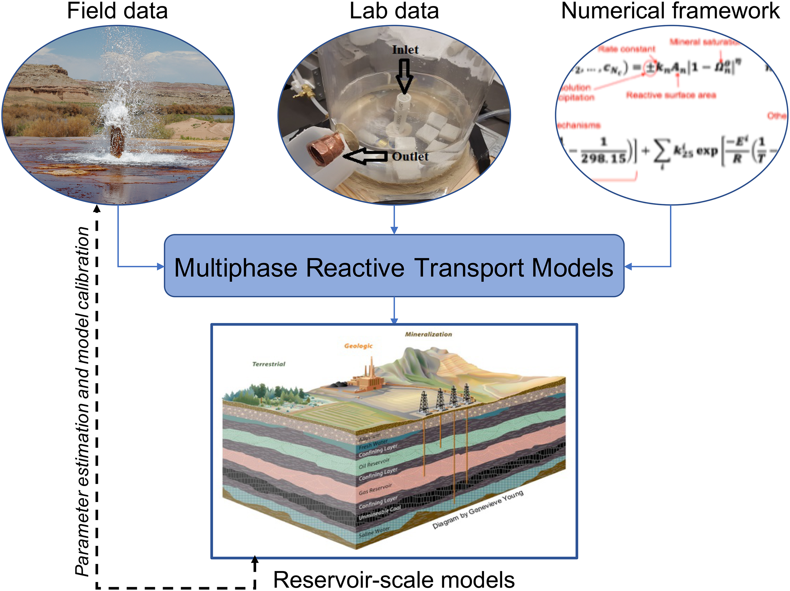
Schematic of an ideal reactive transport modeling workflow. Data from field and laboratory measurements and numerical frameworks (e.g., Damköhler number framework) (Patil and McPherson, 2020) from conceptual models are converted to an input parameter set for multiphase reactive transport codes (e.g., TOUGHREACT) (Xu et al., 2012), which yield reservoir-scale models that aim at mimicking or understanding certain hydrological processes in natural or engineered systems. The predictions from these models can then be compared with active field measurements whenever available for calibration of the model to field reality through inverse modeling or other such techniques (e.g., Doherty, 1994).

A couple of areas that were deemed out of scope for this review, chemical-mechanical coupling and multiscale modeling, need to be mentioned as they may hold the key for the future of reactive transport modeling of fault zones.

Reactive fluid transport along the fault can lead to mineralogical changes impacting the mechanical strength of the fault, potentially affecting the character of fault slip in response to earthquakes in the deeper crust (Gratier, 2011; Bense et al., 2013; Yehya and Rice, 2020). This phenomenon is also critical in many engineered geological applications, like EGS, wherein the functionality and efficiency of the operation is dependent on the integrity of the fractured and faulted host rock (Tomac and Sauter, 2018).

The need for understanding and modeling the coupled effects of the geochemical (mineral precipitation/dissolution) and geomechanical (slips or failures) processes have been recognized by recent studies related to CO₂-Enhanced Oil Recovery (Xiao et al., 2020), geologic CO₂ sequestration (Varre et al., 2015; Raza et al., 2016), and EGS (Xiong et al., 2013; Salimzadeh and Nick, 2019). Several recent experimental studies (Fuchs et al., 2019; Harbert et al., 2020) have aimed at recreating and understanding the chemo-mechanical changes that may occur in highly reactive environments such as subsurface CO₂ systems. However, such laboratory testing can be limited by the timescale. On the other hand, the geomechanical inference from field data is mostly of indirect nature (Ilgen et al., 2019). Hence, the mechanics of coupling of geochemical and geomechanical processes is yet to be quantified for reservoir-scale problems, for example, modeling fault zones, is an area of ongoing research.

Multiscale reactive transport modeling aims at overcoming the limitations of modeling at any one scale (e.g., pore scale or REV scale). Reactive fluid flow through fault zones are inherently a multiscale problem, where different processes need to be handled at different scales. One aspect of this area of study is upscaling reactive transport from pore scale (wherein the models are fundamentally more robust and the results are verifiable and more meaningful from a theoretical standpoint) to reservoir scale (wherein the modeled processes are averaged over a certain REV scale but results at this scale are usually more meaningful from a practical standpoint).

Classically, with this approach, the reactive transport processes are solved at the pore scale and then the results are upscaled to a continuum using effective upscaling parameters. However, the approach depends on accurate quantification of these upscaling parameters that are not directly measurable (Lichtner and Kang, 2007). Over the years, it has become computationally viable to build high-resolution model continuum, which may have the same spatial resolution as the pore-scale model and may not need any hypothetical upscaling factors (e.g., Hao et al., 2019). However, an in-depth understanding of the spatial distribution of the heterogeneity will be critical for accurate predictions and is currently a research challenge, as noted by Erfani et al. (2019).

The second aspect of multiscale modeling is representing different-scaled approaches (pore vs. REV scale) in a single model. This approach, although computationally more intensive, allows a refined way to choose to represent different processes with different scales and then couple them so as to receive feedback from each other at each time step (Scheibe et al., 2007; Molins and Knabner, 2019). Apart from imparting a complex structure to the numerical framework that may not be as “user-friendly” for everyone, the main challenge with this approach lies in the availability of experimental data to supplement the added level of complexity to the models. Future research in this direction could be (1) toward standardized software for multiscale reactive transport modeling (similar to the current industry standards like TOUGHREACT (Xu et al., 2012), etc.), and (2) toward creating an extensive experimental database for geochemical and multiphase flow parameters required to develop these hybrid models.

Footnotes

Acknowledgments

The authors thank Dr. Edward M. Trujillo and Dr. Joseph Moore (University of Utah) for several insightful suggestions, and Dr. Weon Shik Han (University of Wisconsin, now at Yonsei University) and his students for their assistance during the field trips to Crystal Geyser.

Author Disclosure Statement

No competing financial interests exist.

Funding Information

The research efforts were funded by the National Science Foundation (Award 1246302).

References

Ahmad

, Wörman

, Bottacin-Busolin

, and Sanchez-Vila

(2015). Reactive transport modeling of leaking CO₂-saturated brine along a fractured pathway. Int. J. Greenhouse Gas Control, 42, 672.

Ahmad

, Wörman

, Sanchez-Vila

, and Bottacin-Busolin

(2016). The role of advection and dispersion in the rock matrix on the transport of leaking CO₂-saturated brine along a fractured zone. Adv. Water Resour. 98, 132.

Aki

(1979). Characterization of barriers on an earthquake fault. J. Geophys. Res. Solid Earth, 84, 6140.

Allis

, Bergfeld

, Moore

, McClure

, Morgan

, Chidsey

, Heath

, and McPherson

(2005). Implications of results from CO₂ flux surveys over known CO₂ systems for long-term monitoring. In Fourth Annual Conference on Carbon Capture and Sequestration DOE/NETL, Pittsburgh, PA, p. 2.

Aydin

(2000). Fractures, faults, and hydrocarbon entrapment, migration and flow. Marine Petroleum Geol. 17, 797.

Bacon

D.H.

, White

M.D.

, and McGrail

B.P.

(2000). Subsurface transport over reactive multiphases (STORM): A general, coupled, nonisothermal multiphase flow, reactive transport, and porous medium alteration simulator, version 2 user's guide. Richland, WA: Pacific Northwest National Lab.

Barree

R.D.

, and Conway

M.W.

(2004). Beyond beta factors: A complete model for Darcy, Forchheimer, and trans-Forchheimer flow in porous media. In SPE Annual Technical Conference and Exhibition. Houston, TX: Society of Petroleum Engineers.

Bené

J.E.

(2000). Non-Darcy Flow Through Porous Media. Austin, TX: The University of Texas at Austin.

Bense

V.F.

, Gleeson

, Loveless

S.E.

, Bour

, and Scibek

(2013). Fault zone hydrogeology. Earth Sci. Rev. 127, 171.

10.

Berkowitz

(2002). Characterizing flow and transport in fractured geological media: a review. Adv. Water Resour. 25, 861.

11.

Berkowitz

, and Zhou

(1996). Reactive solute transport in a single fracture. Water Resour. Res. 32, 901.

12.

Berner

R.A.

(1978). Rate control of mineral dissolution under earth surface conditions. Am. J. Sci. 278, 1235.

13.

Berner

R.A.

, and Morse

J.W.

(1974). Dissolution Kinetics of calcium carbonate in sea water; IV, theory of calcite dissolution. Am. J. Sci. 274, 108.

14.

Berryman

J.G.

, and Blair

S.C.

(1987). Kozeny–Carman relations and image processing methods for estimating Darcy's constant. J. Appl. Phys. 62, 2221.

15.

Bethke

C.M.

(2008). Geochemical and Biogeochemical Reaction Modelling. Cambridge, UK: Cambridge University Press.

16.

Bodvarsson

G.S.

, Boyle

, Patterson

, and Williams

(1999). Overview of scientific investigations at Yucca mountain—the potential repository for high-level nuclear waste. J. Contam. Hydrol. 38, 3.

17.

Bredehoeft

J.D.

(1997). Fault permeability near Yucca mountain. Water Resour. Res. 33, 2459.

18.

Burnside

N.M.

(2010). U-Th Dating of Travertines on the Colorado Plateau: Implications for the Leakage of Geologically Stored CO₂. Glasgow, SC: University of Glasgow.

19.

Burnside

N.M.

, Shipton

Z.K.

, Dockrill

, and Ellam

R.M.

(2013). Man-made versus natural CO₂ leakage: A 400 k.y. history of an analogue for engineered geological storage of CO₂. Geology, 41, 471.

20.

Busch

, Kampman

, Hangx

S.J.

, Snippe

, Bickle

, Bertier

, Chapman

, Spiers

C.J.

, Pijnenburg

, Samuelson

, Evans

J.P.

, Maskell

, Nicholl

, Pipich

, Di

, Rother

, and Schaller

(2014). The green river natural analogue as a field laboratory to study the long-term fate of CO₂ in the subsurface. Energy Procedia, 63, 2821.

21.

Caine

J.S.

, Evans

J.P.

, and Forste

C.B.

(1996). Fault zone architecture and permeability structure. Geology, 11, 1025.

22.

Carroll

, Mroczek

, Alai

, and Ebert

(1998). Amorphous silica precipitation (60 to 120°C): Comparison of laboratory and field rates. Geochim. Cosmochim. Acta, 62, 1379.

23.

Chambers

J.E.

, Wilkinson

P.B.

, Wealthall

G.P.

, Loke

M.H.

, Dearden

, Wilson

, Allen

, and Ogilvy

R.D.

(2010). Hydrogeophysical imaging of deposit heterogeneity and groundwater chemistry changes during DNAPL source zone bioremediation. J. Contam. Hydrol. 118, 43.

24.

Chen

, Falta

R.W.

, and Murdoch

L.C.

(2015). Numerical analysis of thermal remediation in 3D field-scale fractured geologic media. Groundwater, 53, 572.

25.

Chilingar

G.V.

(1964). Relationship between porosity, permeability, and grain-size distribution of sands and sandstones. In L.M.J.U. van Straaten, Ed., Developments in Sedimentology. Amsterdam, NL: Elsevier, 1, p. 71.

26.

Clement

T.P.

, Sun

, Hooker

B.S.

, and Petersen

J.N.

(1998). Modeling multispecies reactive transport in ground water. Groundwater Monit. Remediation, 18, 79.

27.

Costa

(2006). Permeability-porosity relationship: A reexamination of the Kozeny-Carman equation based on a fractal pore-space geometry assumption. Geophys. Res. Lett. 33.

28.

Crawford

B.R.

, Myers

R.D.

, Woronow

, Faulkner

D.R.

, and Rutter

E.H.

(2002). Porosity-permeability relationships in clay-bearing fault gouge. In SPE/ISRM Rock Mechanics Conference. Irving, TX: Society of Petroleum Engineers.

29.

Delshad

, Asakawa

, Pope

G.A.

, and Sepehrnoori

(2002). Simulations of chemical and microbial enhanced oil recovery methods. In SPE/DOE Improved Oil Recovery Symposium. Tulsa, OK: Society of Petroleum Engineers.

30.

Deng

, Molins

, Trebotich

, Steefel

, and DePaolo

(2018a). Pore-scale numerical investigation of the impacts of surface roughness: Upscaling of reaction rates in rough fractures. Geochim. Cosmochim. Acta, 239, 374.

31.

Deng

, and Spycher

(2019). Modeling reactive transport processes in fractures. Rev. Mineral. Geochem. 85, 49.

32.

Deng

, Steefel

, Molins

, and DePaolo

(2018b). Fracture evolution in multimineral systems: The role of mineral composition, flow rate, and fracture aperture heterogeneity. ACS Earth Space Chem. 2, 112.

33.

Detwiler

R.L.

, and Rajaram

(2007). Predicting dissolution patterns in variable aperture fractures: Evaluation of an enhanced depth-averaged computational model. Water Resour. Res. 43, W04403.

34.

Dockrill

, and Shipton

Z.K.

(2010). Structural controls on leakage from a natural CO₂ geologic storage site: Central Utah, U.S.A. J. Struct. Geol. 32, 1768.

35.

Doherty

(1994). PEST: A unique computer program for model-independent parameter optimisation. Water Down Under 94: Groundwater/Surface Hydrology Common Interest Papers; Preprints of Papers, p. 551.

36.

Domenico

P.A.

, and Schwartz

F.W.

(1990). Physical and Chemical Hydrogeology. New York: Wiley, p. 824.

37.

Ehrenberg

S.N.

, and Nadeau

P.H.

(2005). Sandstone vs. carbonate petroleum reservoirs: A global perspective on porosity-depth and porosity-permeability relationships. AAPG Bull., 89, 435.

38.

Erfani

, Joekar-Niasar

, and Farajzadeh

(2019). Impact of microheterogeneity on upscaling reactive transport in geothermal energy. ACS Earth Space Chem. 3, 2045.

39.

Evans

J.P.

, Heath

, Shipton

Z.K.

, Kolesar

P.T.

, Dockrill

, Williams

, Kirchner

, Lachmar

T.E.

, and Nelson

S.T.

(2004). Natural leaking CO₂-charged systems as analogs for geologic sequestration sites. In Third Annual Conference on Carbon Capture and Sequestration, Alexandria, VA.

40.

Faulkner

D.R.

, Jackson

C.A.L.

, Lunn

R.J.

, Schlische

R.W.

, Shipton

Z.K.

, Wibberley

C.A.J.

, and Withjack

M.O.

(2010). A review of recent developments concerning the structure, mechanics and fluid flow properties of fault zones. J. Struct. Geol. 32, 1557.

41.

Finsterle

(1999). ITOUGH2 user's guide. LBNL-40040. Berkeley, CA: Lawrence Berkeley National Laboratory, 130.

42.

Flewelling

, Matthew

, Tymchak

, and Warpinski

(2013). Hydraulic fracture height limits and fault interactions in tight oil and gas formations. Geophys. Res. Lett. 40. 3602.

43.

Fogler

H.S.

(1992). Elements of Chemical Reaction Engineering. Englewood Cliffs, NJ: Prentice Hall, Inc.

44.

Fossen

(2020). Chapter 8—Fault classification, fault growth and displacement. In N. Scarselli, J. Adam, D. Chiarella, D.G. Roberts, and A.W. Bally, Eds., Regional Geology and Tectonics, 2nd ed. Amsterdam, NL: Elsevier, p. 119. DOI: 10.1016/B978-0-444-64134-2.00007-9.

45.

Fox

F.G.

(1959). Structure and accumulation of hydrocarbons in southern foothills, Alberta, Canada. AAPG Bull. 43, 992.

46.

Fredd

C.N.

, and Fogler

H.S.

(1998). Influence of transport and reaction on wormhole formation in porous media. AIChE J. 44, 1933.

47.

Fuchs

S.J.

, Espinoza

D.N.

, Lopano

C.L

, Akono

A.-T.

, and Werth

C.J.

(2019). Geochemical and geomechanical alteration of siliciclastic reservoir rock by supercritical CO₂-saturated brine formed during geological carbon sequestration. Int. J. Greenhouse Gas Control, 88, 251.

48.

Garven

, Appold

M.S.

, Toptygina

V.I.

, and Hazlett

T.J.

(1999). Hydrogeologic modeling of the genesis of carbonate-hosted lead-zinc ores. Hydrogeol. J. 7, 108.

49.

Gerke

H.H.

, and Van Genuchten

M.T.

(1993). A dual-porosity model for simulating the preferential movement of water and solutes in structured porous media. Water Resour. Res. 29, 305.

50.

Gherardi

, Xu

, and Pruess

(2007). Numerical modeling of self-limiting and self- enhancing caprock alteration induced by CO₂ storage in a depleted gas reservoir. Chem. Geol. 244, 103.

51.

Glassley

W.E.

(2014). Geothermal Energy: Renewable Energy and the Environment. Boca Raton, FL: CRC Press.

52.

Goldhaber

M.B.

, Reynolds

R.L.

, and Rye

R.O.

(1983). Role of fluid mixing and fault-related sulfide in the origin of the Ray Point uranium district, South Texas. Econ. Geol. 78, 1043.

53.

Goyal

K.P.

, and Kassoy

D.R.

(1980). Fault zone controlled charging of a liquid-dominated geothermal reservoir. J. Geophys. Res. Solid Earth, 85, 1867.

54.

Gratier

J.-P.

(2011). Fault permeability and strength evolution related to fracturing and healing episodic processes (years to millennia): The role of pressure solution. Oil Gas Sci. Technol. 66, 491.

55.

Han

W.S.

, Lu

, McPherson

B.J.

, Keating

E.H.

, Moore

, Park

, Watson

Z.T.

, and Jung

N.-H.

(2013). Characteristics of CO₂-driven cold-water geyser, crystal geyser in Utah: Experimental observation and mechanism analyses. Geofluids, 13, 283.

56.

Hao

, Smith

M.M.

, and Carroll

S.A.

(2019). Multiscale modeling of CO₂-induced carbonate dissolution: From core to meter scale. Int. J. Greenhouse Gas Control, 88, 272.

57.

Harbert

, Goodman

, Spaulding

, Haljasmaa

, Crandall

, Sanguinito

, Kutchko

, Tkach

, Fuchs

, and Werth

C.J.

(2020). CO₂ induced changes in Mount Simon sandstone: understanding links to post CO₂ injection monitoring, seismicity, and reservoir integrity. Int. J. Greenhouse Gas Control, 100, 103109.

58.

Heath

J.E.

, Lachmar

T.E.

, Evans

J.P.

, Kolesar

P.T.

, and Williams

A.P.

(2009). Hydrogeochemical characterization of leaking, carbon dioxide-charged fault zones in East-Central Utah, with implications for geologic carbon storage. In Carbon Sequestration and Its Role in the Global Carbon Cycle. Washington, DC: American Geophysical Union, p. 147. DOI: 10.1029/2006GM00, 0407.

59.

Helgeson

H.C.

, Murphy

W.M.

, and Aagaard

(1984). Thermodynamic and kinetic constraints on reaction rates among minerals and aqueous solutions. II. Rate constants, effective surface area, and the hydrolysis of feldspar. Geochim. Cosmochim. Acta, 48, 2405.

60.

Herman

J.S.

, and Lorah

M.M.

(1987). CO₂ outgassing and calcite precipitation in falling spring creek, Virginia, U.S.A. Chem. Geol. 62, 251.

61.

Hoefner

M.L.

, and Fogler

H.S.

(1988). Pore evolution and channel formation during flow and reaction in porous media. AIChE J. 34, 45.

62.

Hong

J.-M.

, Chen

Y.-F.

, Liu

M.M.

, and Zhou

C.-B.

(2017). Inverse modelling of groundwater flow around a large-scale underground cavern system considering the excavation-induced hydraulic conductivity variation. Comput. Geotechnics, 81, 346.

63.

Hood

J.W.

, and Patterson

D.J.

(1984). Bedrock aquifers in the northern San Rafael Swell area, Utah, with special emphasis on the Navajo Sandstone. No. 78. Utah Department of Natural Resources, Division of Water Rights.

64.

Ilgen

A.G.

, Newell

, Hueckel

, Espinoza

D.N.

, and Hu

(2019). Coupled chemical-mechanical processes associated with the injection of CO₂ into subsurface. In P. Newell and A.G. Ilgen, Eds., Science of Carbon Storage in Deep Saline Formations. Cambridge, MA: Elsevier, p. 337.

65.

Ingebritsen

S.E.

, and Sanford

W.E.

(1999). Groundwater in Geologic Processes. New York, NY: Cambridge University Press.

66.

Iskandar

, and Koike

(2011). Distinguishing potential sources of arsenic released to groundwater around a fault zone containing a mine site. Environ. Earth Sci. 63, 595.

67.

Itoi

, Kumamoto

, Tanaka

, and Takayama

(2010). History matching simulation of the ogiri geothermal field, Japan. In Proceedings World Geothermal Congress, Bali, Indonesia.

68.

Jacobs

M.B.

, and Kerr

P.F.

(1965). Hydrothermal alteration along the Lisbon valley fault zone, San Juan County, Utah. GSA Bull. 76, 423.

69.

Jing

, and Stephansson

(2007). 10—Discrete fracture network (DFN) method. In L. Jing and O. Stephansson, Eds., Fundamentals of Discrete Element Methods for Rock Engineering, Developments in Geotechnical Engineering. Amsterdam, NL: Elsevier, 85, p. 365. DOI: 10.1016/S0165-1250(07)85010-3.

70.

Jung

N.-H.

, Han

W.S.

, Watson

Z.T.

, Graham

J.P.

, and Kim

K.-Y.

(2014). Fault-controlled CO₂ leakage from natural reservoirs in the Colorado plateau, East-Central Utah. Earth Planet. Sci. Lett. 403, 358.

71.

Kampman

, Bickle

M.J.

, Maskell

M.J.

, Chapman

H.J.

, Evans

J.P.

, Purser

, Zhou

, Gattacceca

, Schaller

, Bertier

, Chen

, Turchyn

A.S.

, Assayag

, Rochelle

, and Busch

(2014). Drilling and sampling a natural CO₂ reservoir: Implications for fluid flow and CO₂-fluid–rock reactions during CO₂ migration through the overburden. Chem. Geol. 369, 51.

72.

Khoei

A.R.

, Sichani

A.S.

, and Hosseini

(2020). Modeling of reactive acid transport in fractured porous media with the extended–FEM based on Darcy-Brinkman-Forchheimer framework. Comput. Geotechnics, 128, 103778.

73.

Kiryukhin

, Xu

, Pruess

, Apps

, and Slovtsov

(2004). Thermal–hydrodynamic–chemical (THC) modeling based on geothermal field data. Geothermics, 33, 349.

74.

Knipe

R.J.

, Jones

, and Fisher

Q.J.

(1998). Faulting, fault sealing and fluid flow in hydrocarbon reservoirs: An introduction. Geol. Soc. London Spl. Publ. 147, vii.

75.

Lachhab

, Benyassine

E.M.

, Rouai

, Dekayir

, Parisot

J.C.

, and Boujamaoui

(2020). Integration of multi-geophysical approaches to identify potential pathways of heavy metals contamination-A case study in Zeida, Morocco. J. Environ. Eng. Geophys. 25, 415.

76.

Lage

(1998). The fundamental theory of flow through permeable Niedia from Darcy to turbulence. In D.B. Ingham, and I. Pop, Eds., Transport Phenomena in Porous Media. Pergamon, Oxford, UK, p. 1.

77.

Lai

, Moulton

, and Krevor

(2015). Pore-scale heterogeneity in the mineral distribution and reactive surface area of porous rocks. Chem. Geol. 411, 260.

78.

Landrot

, Ajo-Franklin

J.B.

, Yang

, Cabrini

, and Steefel

C.I.

(2012). Measurement of accessible reactive surface area in a sandstone, with application to CO₂ mineralization. Chem. Geol. 318, 113.

79.

Larsson

M.H.

, and Jarvis

N.J.

(1999). A dual-porosity model to quantify macropore flow effects on nitrate leaching. J. Environ. Qual. 28, 1298.

80.

Lasaga

A.C.

(1981). Rate laws of chemical reactions. Rev. Mineral. (United States), 8, 1.

81.

Lasaga

A.C.

(1984). Chemical kinetics of water-rock interactions. J. Geophys. Res. 89, 4009.

82.

Lasaga

A.C.

(1995). Fundamental approaches in describing mineral dissolution and precipitation rates. Rev. Miner. Geochem. 31, 23.

83.

Lasaga

A.C.

(1998). Kinetic Theory in the Earth Sciences. Princeton, NJ: Princeton University Press.

84.

Lasaga

A.C.

, Soler

J.M.

, Ganor

, Burch

T.E.

, and Nagy

K.L.

(1994). Chemical weathering rate laws and global geochemical cycles. Geochim. Cosmochim. Acta, 58, 2361.

85.

Lee

, Choi

S.-U.

, and Cho

(1999). A comparative study of dual-porosity model and discrete fracture network model. KSCE J. Civil Eng. 3, 171.

86.

Levenspiel

(1999). Chemical reaction engineering. Ind. Eng. Chem. Res. 38, 4140.

87.

Lichtner

P.C.

(1996). Continuum formulation of multicomponent-multiphase reactive transport. Rev. Miner. Geochem. 34, 1.

88.

Lichtner

P.C.

, and Kang

(2007). Upscaling pore-scale reactive transport equations using a multiscale continuum formulation. Water Resour. Res. 43, W12S15.

89.

MacQuarrie

K.T.B.

, and Ulrich Mayer

(2005). Reactive transport modeling in fractured rock: A state-of- the-science review. Earth Sci. Rev. 72, 189.

90.

Matthäi

S.K.

(2003). Fluid flow and (reactive) transport in fractured and faulted rock. J. Geochem. Exploration, 78, 179.

91.

May

(2005). Alteration of wall rocks by CO₂-rich water ascending in fault zones: Natural analogues for reactions induced by CO₂ migrating along faults in siliciclastic reservoir and cap rocks. Oil Gas Sci. Technol. 60, 19.

92.

Mayer

, May

, Lukkarila

, and Diehl

(2007). Estimation of fault-zone conductance by calibration of a regional groundwater flow model: Desert Hot Springs, California. Hydrogeol. J. 15, 1093.

93.

Mercer

J.W.

, Cohen

R.M.

, and Noel

M.R.

(2010). DNAPL site characterization issues at chlorinated solvent sites. In H.F. Stroo and C.H. Ward, Eds., In Situ Remediation of Chlorinated Solvent Plumes. New York, NY: Springer, p. 217.

94.

Molins

(2015). Reactive interfaces in direct numerical simulation of pore-scale processes. Rev. Mineral. Geochem. 80, 461.

95.

Molins

, and Knabner

(2019). Multiscale approaches in reactive transport modeling. Rev. Mineral. Geochem. 85, 27.

96.

Molins

, Trebotich

, Yang

, Ajo-Franklin

J.B.

, Ligocki

T.J.

, Shen

, and Steefel

C.I.

(2014). Pore-scale controls on calcite dissolution rates from flow-through laboratory and numerical experiments. Environ. Sci. Technol. 48, 7453.

97.

Moore

, McLennan

, Allis

, Pankow

, Simmons

, Podgorney

, Wannamaker

, and Pickard

(2018). The Utah Frontier Observatory for Geothermal Research (FORGE): Results of recent drilling and geoscientific surveys. In Geothermal Resources Council 42nd Annual Meeting-Geothermal Energy. Reno, NV: GRC.

98.

Moore

J.N.

, and Simmons

S.F.

(2013). More power from below. Science, 340, 933.

99.

Moretti

(1998). The roles of faults in hydrocarbon migration. Petrol. Geosci. 4, 81.

100.

Murphy

W.M.

, Oelkers

E.H.

, and Lichtner

P.C.

(1989). Surface reaction versus diffusion control of mineral dissolution and growth rates in geochemical processes. Chem. Geol. 78, 357.

101.

Mwetulundila

A.L.

, and Atangana

(2020). Applying the Forchheimer equation to model an artificially recharged fractured aquifer. Alexandria Eng. J. 59, 2115.

102.

Narasimhan

T.N.

, and Pruess

(1988). Minc: An approach for analyzing transport in strongly heterogeneous systems. In E. Custodio, A. Gurgui, and J.P. Lobo Ferreira, Eds., Groundwater Flow and Quality Modelling. Dordrecht, NL: Springer, p. 375.

103.

Nelson

P.H.

(1994). Permeability-porosity relationships in sedimentary rocks. Log Anal. 35.

104.

Orellana

, Felipe

, Giorgetti

, and Violay

(2019). Contrasting mechanical and hydraulic properties of wet and dry fault zones in a proposed shale-hosted nuclear waste repository. Geophys. Res. Lett. 46, 1357.

105.

Palandri

J.L.

, and Kharaka

Y.K.

(2004). A compilation of rate parameters of water-mineral interaction kinetics for application to geochemical modeling. DTIC Document. Menlo Park, CA: US Geological Survey.

106.

Parkhurst

D.L.

, and Appelo

C.A.J.

(1999). User's guide to PHREEQC (version 2): A computer program for speciation, batch-reaction, one-dimensional transport, and inverse geochemical calculations. Water-resources investigations report, 99(4259), 312.

107.

Patil

V.V.

(2016). Self-sealing of faults in geological carbon sequestration. Salt Lake City, UT: University of Utah.

108.

Patil

V.V.

, and McPherson

B.J.

(2020). Identifying hydrogeochemical conditions for fault self-sealing in geological CO₂ storage. Water Resour. Res. 56, e2018WR024436.

109.

Patil

V.V.

, McPherson

B.J.

, Priewisch

, Moore

, and Moodie

(2017). Factors affecting self-sealing of geological faults due to CO₂-leakage. Greenhouse Gases Sci. Technol. 7, 273.

110.

Patil

V.V.

, and Simmons

(2020). Evaluation of potential geochemical responses to injection in the forge geothermal reservoir. Utah. Report 1247. Available at: http://gdr.openei.org/submissions/1247 (accessed September 8, 2020).

111.

Raleigh

C.B.

, Healy

J.H.

, and Bredehoeft

J.D.

(1972). Faulting and Crustal stress at Rangely, Colorado. GMS, 16, 275.

112.

Raza

, Gholami

, Sarmadivaleh

, Tarom

, Rezaee

, Bing

C.H.

, Nagarajan

, Hamid

M.A.

, and Elochukwu

(2016). Integrity analysis of CO₂ storage sites concerning geochemical-geomechanical interactions in saline aquifers. J. Natural Gas Sci. Eng. 36, 224.

113.

Rotevatn

, and Fossen

(2011). Simulating the effect of subseismic fault tails and process zones in a siliciclastic reservoir analogue: Implications for aquifer support and trap definition. Mar. Petroleum Geol. 28, 1648.

114.

Rufe

, and Hochella

M.F.

(1999). Quantitative assessment of reactive surface area of phlogopite during acid dissolution. Science, 285, 874.

115.

Salimzadeh

, and Nick

H.M.

(2019). A coupled model for reactive flow through deformable fractures in enhanced geothermal systems. Geothermics, 81, 88.

116.

Scheibe

T.D.

, Tartakovsky

A.M.

, Tartakovsky

D.M.

, Redden

G.D.

, and Meakin

(2007). Hybrid numerical methods for multiscale simulations of subsurface biogeochemical processes. J. Phys. Conf. Ser. 78, 12063.

117.

Shipton

Z.K.

, Evans

J.P.

, Dockrill

, Heath

, Williams

, Kirchner

, and Kolesar

P.T.

(2005). Chapter 4—Natural leaking CO₂-charged systems as analogs for failed geologic storage reservoirs. In D.C. Thomas, and S.M. Benson, Eds., Carbon Dioxide Capture for Storage in Deep Geologic Formations. Amsterdam: Elsevier Science, p. 699.

118.

Siirila

E.R.

, Navarre-Sitchler

A.K.

, Maxwell

R.M.

, and McCray

J.E.

(2012). A quantitative methodology to assess the risks to human health from CO₂ leakage into groundwater. Adv. Water Resour. 36, 146.

119.

Simmons

, Kirby

, Allis

, Moore

, and Fischer

(2018). Update on production chemistry of the Roosevelt Hot Springs reservoir. In 43rd Workshop on Geothermal Reservoir Engineering Stanford University. Stanford, California: Stuart F Simmons/University of Utah.

120.

Smith

D.A.

(1966). Theoretical considerations of sealing and non-sealing faults. AAPG Bull. 50, 363.

121.

Sonnenthal

E.L.

, Torquil Smith

, Cladouhos

, Kim

, and Yang

(2015). Thermal-Hydrological- mechanical-chemical modeling of the 2014 EGS stimulation experiment at Newberry Volcano, Oregon. In Proceedings, Fortieth Workshop on Geothermal Reservoir Engineering. Stanford University, Stanford, CA.

122.

Sorkhabi

R.B.

, and Tsuji

(2005). Faults, fluid flow, and petroleum traps. AAPG Memoir, 85, 1.

123.

Stanley

T.B.

Jr. (1970). Vicksburg fault zone, Texas. In Geology of Giant Petroleum Fields. p. 301.

124.

Steefel

C.I.

, and Lasaga

A.C.

(1994). A coupled model for transport of multiple chemical species and kinetic precipitation/dissolution reactions with application to reactive flow in single phase hydrothermal systems. Am. J. Sci. 294, 529.

125.

Takhanov

(2011). Forchheimer model for non-Darcy flow in porous media and fractures. London, UK: Imperial College London.

126.

Talbot

M.S.

, and Gdanski

R.D.

(2008). Beyond the Damkohler number: A new interpretation of carbonate wormholing. In Europec/EAGE Conference and Exhibition. Rome, IT: Society of Petroleum Engineers.

127.

Taron

, and Elsworth

(2009). Thermal–hydrologic–mechanical–chemical processes in the evolution of engineered geothermal reservoirs. Int. J. Rock Mech. Mining Sci. 46, 855.

128.

Tian

, Xu

, Wang

, Patil

V.V.

, Sun

, and Yue

(2014). A numerical study of mineral alteration and self-sealing efficiency of a caprock for CO₂ geological storage. Acta Geotech. 9, 87.

129.

Tomac

, and Sauter

(2018). A review on challenges in the assessment of geomechanical rock performance for deep geothermal reservoir development. Renew. Sustain. Energy Rev. 82, 3972.

130.

Varre

S.B.K.

, Siriwardane

H.J.

, Gondle

R.K.

, Bromhal

G.S.

, Chandrasekar

, and Sams

(2015). Influence of geochemical processes on the geomechanical response of the overburden due to CO₂ storage in saline aquifers. Int. J. Greenhouse Gas Control, 42, 138.

131.

Vrolijk

, Myers

, Sweet

M.L.

, Shipton

Z.K.

, Dockrill

, Evans

J.P.

, Heath

, and Williams

A.P.

(2005). Anatomy of reservoir-scale normal faults in Central Utah: Stratigraphic controls and implications for fault zone evolution and fluid flow. Field Guides, 6, 261.

132.

Warren

J.E.

, and Root

P.J.

(1963). The behavior of naturally fractured reservoirs. Soc. Petroleum Eng. J. 3, 245.

133.

White

M.D.

, and Oostrom

(2003). STOMP subsurface transport over multiple phases version 3.0 user's guide. Richland, WA: Pacific Northwest National Lab.

134.

Wilkinson

J.J.

, Stoffell

, Wilkinson

C.C.

, Jeffries

T.E.

, and Appold

M.S.

(2009). Anomalously metal-rich fluids form hydrothermal ore deposits. Science, 323, 764.

135.

Xiao

, Xu

, Moodie

, Esser

, Jia

, Zheng

, Rutqvist

, and McPherson

(2020). Chemical-mechanical impacts of CO₂ intrusion into heterogeneous caprock. Water Resour. Res. e2020WR027193, 1.

136.

Xiong

, Fakcharoenphol

, Winterfeld

, Zhang

, and Wu

Y.-S.

(2013). Coupled Geomechanical and Reactive Geochemical Model for Fluid and Heat Flow: Application for Enhanced Geothermal Reservoir. In SPE Reservoir Characterization and Simulation Conference and Exhibition. Abu Dhabi, UAE: Society of Petroleum Engineers.

137.

(2001). Modeling multiphase non-isothermal fluid flow and reactive geochemical transport in variably saturated fractured rocks: 1. Methodology. Am. J. Sci., 301, 16.

138.

, and Pruess

(2004). Numerical simulation of injectivity effects of mineral scaling and clay swelling in a fractured geothermal reservoir. Berkeley, CA: Lawrence Berkeley National Lab (LBNL).

139.

, Rose

, Fayer

, and Pruess

(2009). On modeling of chemical stimulation of an enhanced geothermal system using a high pH solution with chelating agent. Geofluids, 9, 167.

140.

, Sonnenthal

, and Bodvarsson

(2003). A reaction-transport model for calcite precipitation and evaluation of infiltration fluxes in unsaturated fractured rock. J. Contam. Hydrol. 64, 113.

141.

, Sonnenthal

, Spycher

, and Pruess

(2006). TOUGHREACT—A simulation program for non-isothermal multiphase reactive geochemical transport in variably saturated geologic media: Applications to geothermal injectivity and CO₂ geological sequestration. Comput. Geosci. 32, 145.

142.

, Sonnenthal

, Spycher

, Pruess

, Brimhall

, and Apps

(2001). Modeling multiphase non-isothermal fluid flow and reactive geochemical transport in variably saturated fractured rocks: 2. Applications to supergene copper enrichment and hydrothermal flows. Am. J. Sci., 301, 34.

143.

, Spycher

, Sonnenthal

, Zheng

, and Pruess

(2012). TOUGHREACT user's guide: A simulation program for non-isothermal multiphase reactive transport in variably saturated geologic media, version 2.0. Berkeley, CA: Lawrence Berkeley National Laboratory.

144.

Yang

, and Aplin

A.C.

(2010). A permeability–porosity relationship for mudstones. Marine Petroleum Geol. 27, 1692.

145.

Yeh

G.-T.

, and Tripathi

V.S.

(1991). A model for simulating transport of reactive multispecies components: Model development and demonstration. Water Resour. Res. 27, 3075.

146.

Yehya

, and Rice

J.A.

(2020). Influence of fluid-assisted healing on fault permeability structure. J. Geophys. Res. Solid Earth. 125, e2020JB020553.

147.

Yuan

, Xu

, Moore

, Lei

, and Feng

(2020). Coupled thermo–hydro–mechanical modeling of hydro-shearing stimulation in an enhanced geothermal system in the raft river geothermal field, USA. Rock Mech. Rock Eng. 53, 5371.

148.

Zhang

, Sun

, and Song

(2019). Flow mechanism and simulation approaches for shale gas reservoirs: A review. Transport Porous Media, 126, 655.

149.

Zhang

, Gartrell

, Underschultz

J.R.

, and Dewhurst

D.N.

(2009). Numerical modelling of strain localisation and fluid flow during extensional fault reactivation: Implications for hydrocarbon preservation. J. Struct. Geol. 31, 315.

150.

Zheng

, Apps

J.A.

, Zhang

, Xu

, and Birkholzer

J.T.

(2009). On mobilization of lead and arsenic in groundwater in response to CO₂ leakage from deep geological storage. Chem. Geol. 268, 281.