Municipal Solid Waste Biodegradability and Methane Potential: Influence of Fiber Content and Elemental Composition

Abstract

Managing municipal solid waste (MSW) presents many challenges, including the production of methane when MSW biodegrades in landfills. The search for methods to predict methane generation easily and accurately has been ongoing as MSW management improves and the damage presented by greenhouse gases is realized. To study MSW biodegradability, samples of solid waste were collected by sorting trash at four landfills and transfer stations in the southeast United States and transported to laboratories where the MSW was processed and analyzed for methane potential using biochemical methane potential assay, fiber content (lignin, cellulose, and hemicellulose), total carbon analysis, and elemental analysis. Searches for correlation between these data and methane generation revealed that average cellulose content correlated with methane generation potential (R² = 0.90). A formula for predicting the methane potential of MSW samples using elemental analysis and 1 of 14 different correction factors, assigned by waste category type, is also presented. The methods presented in this work can help researchers and landfill operators better evaluate the methane potential of the MSW they work with.

Introduction

Over 62% of municipal solid waste (MSW) mass entering landfills in the United States can decompose anaerobically to form landfill gas according to annual estimates by the U.S. Environmental Protection Agency (EPA), based on the EPA's definition of MSW (U.S. EPA, 2020). Several factors prevent these nearly 92 million tons of degradable materials from decomposing completely into gaseous products. Successful microbial decomposition requires appropriate environmental conditions, including proper moisture content, temperature, pH, and nutrient availability (Tchobanoglous et al., 1993; Haug, 2018). Inaccessibility to substrates, due to structural shielding by lignin or their complex polymeric forms, can prevent biodegradation (Stinson and Ham, 1995; Hettiaratchi et al., 2014). In this study, biodegradable constituents of MSW are referred to in this work as three simplified “fibers” and are defined as cellulose, hemicellulose, and lignin. These compounds are the major component of each fiber, although traces of other materials (fats, oils, and other polymers) were likely present during analysis.

Cellulose, the most abundant organic compound on Earth, consists of glucose subunits that are readily consumed once the parent compound has been hydrolyzed (Chandler et al., 1980). Hemicellulose is a polysaccharide constructed of five carbon sugars (mostly xylose) with β-1-4 glycosidic linkages, which is accessible for degradation in many MSW materials (Sánchez, 2009). Lignin, a much more complex three-dimensional polymerized aromatic alcohol, is constructed of aromatic rings with strong C-C bonds that require oxidative attack for effective breakdown (Higuchi, 2004). A goal of many researchers has been to quantify how these fibers contribute to anaerobic biodegradability (AB) in landfills and anaerobic digestion systems, both for assessing potential methane production through anaerobic treatment and for measuring the degree of stability achieved during treatment and disposal (Barlaz, 1998; Wang et al., 2013; Bayard et al., 2018).

While cellulose and some hemicellulose components biodegrade with relative ease, lignin is highly resistant to degradation (Eleazer et al., 1997; Sánchez, 2009; Jayasinghe et al., 2011), and has consequently been a focus of much research in the study of MSW and organic waste degradation (Chandler et al., 1980; Stinson and Ham, 1995; Komilis and Ham, 2003; Hettiaratchi et al., 2014). When comparing the degree of AB among substrates, a common assumption is that the material with the highest lignin content will be the least degradable as oxygen is necessary to facilitate the oxidative reactions for breaking lignin's carbon bonds (Sánchez, 2009). Chandler et al. (1980) first described a correlation between the lignin content of volatile solids (VS_lignin) and the anaerobically biodegradable fraction (BF) of volatile solids (VS_{biodegradable}) in agricultural components with Equation (1): $V S_{b i o d e g r a d a b l e} = - 2.8 V S_{l i g n i n} + 0.83$ (1)

Chandler et al. (1980) compared the lignin content of 15 different agricultural products, manures, and newsprint against the VS destruction measured after 120 days of anaerobic batch digestion. While this equation has been applied to MSW, Tchobanoglous et al. (1993) noted that most of the materials comprising current MSW were not included in the experiment on which it is based. A better understanding of the relationship between waste fiber content and biodegradability would benefit both engineers and operators relying on fiber content for estimates of gas production and landfill settlement, as well as those attempting to predict the biodegradability of an evolving MSW stream as related to organic waste management technologies such as anaerobic digestion.

In this study, both the mass of total carbon available in the substrates, determined before biochemical methane potential (BMP) assays, and the calculated mass of carbon evolved to gas as CH₄ and CO₂ in the assays were measured. The fraction of carbon evolved from solid in the substrate to gas was used as the metric for determining AB. This approach is similar to that used by the Intergovernmental Panel on Climate Change (IPCC) Waste Model in defining the parameter DOC_f, a metric for quantifying the fraction of degradable organic carbon (DOC) predicted to evolve anaerobically into a gas (Krause et al., 2016). The IPCC Waste Model's default value for DOC_f is 0.5, meaning half the degradable organic carbon in MSW is expected to degrade under anaerobic conditions. A study of the biodegradability of forest products in landfills found high variability in the decomposition of these materials and suggests the default IPCC value of 50% is an average derived from the wide range of expected degradability in MSW components (Wang, 2015).

With differing approaches for quantifying MSW biodegradability presented in previous studies, the goal of this work was to more closely examine the relationship between measured fiber content and the AB of these specific MSW components using gas production data gathered directly from the same samples. This work compares the results to those studies dominated by agricultural products (Chandler et al., 1980) and prior work that focused on smaller subsets of MSW components. To accomplish this goal, a uniform set of MSW collection methods was employed to obtain a large sample set for fiber content analysis and determination of BMP. The relationship between biodegradability and fiber content is presented in this work.

Another pressing concern in waste management is accurately predicting the potential yield of biogas, particularly methane, from MSW in landfills and anaerobic digestion facilities. The significance of methane is particularly important to waste management in the United States because the country deposits an estimated 92 million tons of biodegradable waste in landfills each year (U.S. EPA, 2020). While average values of ultimate methane generation potential for MSW components have been published previously (Chickering et al., 2018), accurately estimating the potential yields of specific waste components without running lengthy BMP assays would be beneficial. While BMP and similar assays serve a purpose, the time and labor required are often extensive and reflect the upper limit of methane production under ideal conditions (Owen et al., 1979; ASTM E 1196-92, 1992; Eleazer et al., 1997; Holliger et al., 2016).

Accurate assessment of biodegradability in solid samples requires a protocol that incorporates biogas potential assays, defeating the purpose of determining biodegradability as an indicator of yield (Lesteur et al., 2010). Chandler et al. (1980) measured the BF of VS by gravimetrically analyzing VS content before and after 120 days of anaerobic batch digestion. A 2017 characterization of MSW in France not only compared chemical oxygen demand (COD) and 28-day biological oxygen demand in solid samples to assess biodegradability aerobically but also had to resort to 60-day BMP assays to quantify AB (Bayard et al., 2018). Bayard et al.'s (2018) determination of AB by dividing BMP values by COD has been used successfully by other MSW studies as well (Lesteur et al., 2010).

While the ability of a material to biodegrade influences biogas yield, the quantity of gas yield may still not be directly predictable with biodegradability data. One specific method for instantly predicting gas yields is using the chemical formula of the substrate to estimate the quantity of gaseous products that can be generated (Achinas and Euverink, 2016). The stoichiometry of a degradable organic material dictates the potential yield of biogas that the substrate can generate under ideal anaerobic conditions, as one element eventually becomes the limiting reagent. This assumes all environmental conditions allow full degradation.

The basis for most stoichiometric estimates for CH₄ and CO₂ yield was presented by Buswell and Mueller (1952) and modified later by Boyle (1977) to incorporate nitrogen and sulfur (Tchobanoglous et al., 1993). This balanced redox equation is simplified to describe an anaerobic reaction in which an organic compound reacts to form CH₄, CO₂, NH₃, and H₂S (Labatut et al., 2011). This Equation (2) only considers the relative proportions of carbon, hydrogen, oxygen, nitrogen, and sulfur (CHONS), ignoring the other elements present in the substrate. $\begin{matrix} C_{a} H_{b} O_{c} N_{d} S_{e} & + (a - \frac{b}{4} - \frac{c}{2} + \frac{3 d}{4} + \frac{e}{2}) H_{2} O \to (\frac{a}{2} + \frac{b}{8} - \frac{c}{4} - \frac{3 d}{8} - \frac{e}{4}) C H_{4} \\ + (\frac{a}{2} - \frac{b}{8} + \frac{c}{4} + \frac{3 d}{8} + \frac{e}{4}) C O_{2} + d N H_{3} + e H_{2} S \end{matrix}$ (2)

Achinas and Euverink (2016) state that the equations of Buswell and Mueller (1952) as well as Boyle (1977) assume a complete conversion of biodegradable biomass, which will exclude lignin and other recalcitrant organic molecules. The value predicted by this equation is the ultimate quantity of methane a given waste product can produce if all the matter it contained were biodegradable and converted into the gases of interest (Lesteur et al., 2010). Considering that it is logistically impossible to separate VS from non-VS before elemental analysis of dry organic waste, empirical formulas determined for this work represent the entire mass of substrate, including nonmethane yielding lignin. Recalcitrant masses of lignin and nonbioavailable substrates are partially responsible for lower observed yields relative to stoichiometric predictions (Komilis and Ham, 2003; Lesteur et al., 2010, 2011). Additional factors that reduce the observed yield include adverse environmental conditions (temperature, moisture content, oxygen presence, etc.) and the nutritional requirements of the microorganisms catabolizing the substrate under study, which convert some substrate into microbial biomass (Labatut et al., 2011; Krause et al., 2016).

Substrates almost never reach their ultimate yield predicted by stoichiometry, as the microorganisms degrading the materials incorporate carbon, nitrogen, sulfur, and other elements into their own biomass, while expelling gaseous byproducts throughout their catabolic processes. Other hindrances include complex polymers such as lignin and other resilient structures that cannot be broken down by most suites of microbes and remain as recalcitrant mass (Chandler et al., 1980; Chen, 2014). Because of these differences in observed and predicted yields, several researchers have attempted to create correction factors to pair with stoichiometric estimates. Achinas and Euverink (2016) proposed a limiting factor of 0.8 to be applied to all estimates using a simplified version of the Buswell equation in a study of agricultural waste products. When using the IPCC's Waste Model, a tool designed to predict methane potential of MSW, a parameter termed the fraction of anaerobically decomposable DOC (DOC_f) is included with a default value of 0.5 to be applied to general MSW (Pipatti and Svardal, 2006). While these and other limiting/correction factors were determined through differing approaches, the practice of applying similar corrections to specified components of MSW appears to be a novel practice.

To better predict the MSW methane potential using stoichiometric estimates, this work presents an adaptation of the Buswell equation with 14 new correction factors, 1 for each of the 14 categories of MSW studied. The correction factors are based on this work's method presented for quantifying AB, using total carbon content and gas production in BMP assays, all performed on the same samples to allow direct comparison. In addition, findings presented suggest that if elemental analysis is not possible, measuring fiber content with the streamlined method employed in this study can be used to predict methane potential accurately. These findings and improvements extend the work of many researchers to provide new tools for scientists and operators to estimate MSW gas production.

Materials and Methods

Approach

The three main efforts of this research were to assess fiber content in MSW components, perform elemental analysis on a subset of samples, and quantify biodegradability using BMP assays so these data could all be paired to predict methane generation potential. Lignin content, along with cellulose, hemicellulose, ash, and soluble fraction content were analyzed using the Ankom 200 Fiber Analysis system (Ankom). Biodegradability was quantified by assessing the total carbon content of the different waste component substrates (which was assumed to be predominately organic carbon), measuring the amount CH₄ and CO₂ generated in each BMP bottle, and calculating the fraction of carbon that evolved phase under anaerobic conditions. In this research, the fraction of carbon that mineralized to gas (CO₂ and CH₄) was assumed to be the same as the fraction of mass that can biodegrade (Buffiere et al., 2006; Lesteur et al., 2010). While a small mass of carbon could have dissolved into the growth media as CO₂ or been absorbed as biomass by methanogens, these losses were assumed to be negligible relative to the volume of gas produced in each BMP assay bottle. The average CHONS compositions of 14 different MSW fractions were analyzed, and methane yields were predicted using the Buswell equation and compared against observed methane yields from the same samples, obtained through BMP assays. The accuracy of the predictions relative to observed yields is assessed and potential influences on accuracy were investigated.

Sample collection and BMP assays

Eighty samples of MSW components were collected at their points of disposal with the goal of obtaining substrates with most of their methane generation potential still intact. Four abridged waste composition studies were performed at landfills, transfer stations, and waste-to-energy facilities in Florida, Georgia, and North Carolina. While 42 total categories were used for the sorting process, 14 types of MSW were collected and transported to the Solid and Hazardous Waste Laboratories at the University of Florida (Gainesville, FL) for further analysis. These methods, including sorting procedures and sample analysis, are further described in a previous study that focused specifically on the ultimate methane potential of these MSW components (Chickering et al., 2018). These similar MSW samples were analyzed for elemental composition and fiber content in this study.

The fractions of MSW used for this study are listed in Table 1. Most of the categories are self-explanatory; however, two fractions are identified as the biodegradable fines fraction (BFF) that passed through a sorting table screen, referred to in this study as BFF <5 cm² and BFF <2.5 cm². The fines fractions are composed of materials too small to sort efficiently, although they contribute significantly to methane production in landfills. These materials were collected after falling through the top screen (∼5 cm²) and bottom screen (∼2.5 cm²) of the sorting table used for the waste composition study. The label BFF refers to the biodegradable fines fraction, which is the material perceived to be biodegradable in the fines samples. The BFF was created in the laboratory when each fines sample was sorted on a bench into materials perceived to be biodegradable (BFF) and those assumed to be inert fines fraction (IFF). This sorting reduced wear on processing equipment and reduced ash content when determining VS content. BMP assays were completed as described in Chickering et al. (2018).

Table 1.

Comparison of Findings in This Study with Published Fiber Content Analysis in Relevant Samples Using Various Methods

Source	Analysis method	Sample	Soluble, %	Cellulose, %	Hemicellulose, %	Lignin, %	Ash, %
This study	Ankom 200	Cardboard	18	57	9	14	3
		Newspaper	14	45	14	24	2
		Office paper	25	59	5	10	1
		Pasteboard	16	61	7	12	4
		Junk mail	24	56	6	12	1
		Aseptic paper	13	53	10	23	1
		Misc. paper	23	54	9	12	3
		Food waste	46	25	21	7	3
		Yard waste	26	33	15	21	5
		BF fines <5 cm	34	31	14	16	6
		BF fines <2.5 cm	49	12	21	11	8
		Textile	11	72	2	14	1
		Wood	10	50	12	26	1
		Comp wood	14	46	19	20	0
Komilis and Ham (2003)	HPLC	Office paper	4	68	7	7
		Food waste	27	46	0	12
		Yard waste	24	27	11	24
Bayard et al. (2016)	Van Soest method	Food waste	51	12	28	9
		Mix of green waste	37	18	16	29
		Fines fraction	56	20	14	10
		Newsprints	9	74	9	9
		Office paper	19	77	2	2
		Magazines	11	87	1	1
		Corrugated board	18	54	12	17
		Cotton textiles	15	80	1	4
		Sanitary textiles	0	81	15	4
		Diapers	0	67	0	33
		Wood	5	50	15	30
		Composites	20	39	21	20
Chandler et al. (1980)	Van Soest method	Newsprint	11			21
Eleazer et al. (1997)	HPLC	Coated paper		42	9	15
		Old newsprint		49	9	24
		Corrugated board		57	10	21
		Office paper		87	8	2
		Food waste		55	7	11
		Branch		35	18	33
		Leaves		15	11	44
		Grass		27	10	28
Wang et al. (2013)	HPLC	Plywood		39	17	31
		Particle board		37	16	28
		Medium density fiberboard		35	15	30
		Newsprint		53	15	14
		Copy paper		70	14	1
		Corrugated board		62	15	14

“Soluble” represents the fraction of plant cells that is soluble in the first neutral detergent wash of the Van Soest and Aknom protocols. Values determined using this study's Ankom 200 method represent averages of six samples (two for composite wood) that were all tested in triplicate. Values are in dry mass fiber/dry mass total sample.

BF, biodegradable fraction; Comp, composite; HPLC, high-performance liquid chromatography.

Fiber analysis

The dried, ground samples were analyzed for lignin, cellulose, hemicellulose, ash, and soluble component content using an Ankom 200 fiber analyzer and the manufacturer's standard methods (Anokm). Each dried sample was first subjected to a neutral detergent fiber digestion solution that removes soluble components, including pectin, gums, lipids, oils, waxes, and other nonpolar extracts (Chandler et al., 1980; Lewis, 2005; Bayard et al., 2016). Hemicellulose and some hemicellulose-bound proteins were removed with a dilute acidic aqueous detergent solution (Lewis, 2005). After hemicellulose was removed, the remaining fiber was digested in 72% H₂SO₄, which removes cellulose, but leaves lignin, cutin, and ash behind (Chandler et al., 1980). A final combustion at 550°C in a muffle furnace removes the remaining organic matter (lignin) and leaves dry ash remaining in the combustion vessel. In this study, these categories are simplified and labeled as soluble components, hemicellulose, cellulose, lignin, and ash.

Total carbon analysis

The dried, ground, homogenized samples were analyzed for total carbon content at the University of Florida Institute of Food and Agricultural Sciences (UF-IFAS) Extension Soil Testing Laboratory. All 80 samples (∼5 g each) were analyzed for total carbon content using an Elementar vario MACRO cube elemental analyzer (Elementar, Germany).

Calculation of biodegradability

Biodegradability was quantified in this study by analyzing the total mass of carbon in the dry, ground, homogenized samples and comparing that to the mass of carbon present in CO₂ and CH₄ evolved from each respective substrate in the BMP assays. The process for this calculation is detailed in Equations (3–6). Chandler et al. (1980) used the term VS_{biodegrabable} to describe biodegradability, referring specifically to the mass of original substrate VS destroyed in an anaerobic batch reactor. For ease of comparison, the term AB is used in this study to describe degradability of these samples and also represents the term VS_{biodegrabable}.

In Equation (3), C = carbon mass in dry sample (g), M = total sample mass (g), and C_% = % carbon in dry sample. In Equation (4), C_CH4 = carbon mass in CH₄ (g)_, VS = mass of substrate volatile solids (g) added to assay bottle, and BMP stands for the milliliter of gas measured in the BMP assay at standard temperature and pressure (STP) (1 ATM, 0°C). In Equation (5), C_CO2 = carbon mass in CO₂ (g) and VS = mass of substrate volatile solids (g) added to assay bottle. In Equation (6), AB represents anaerobic biodegradability, C_CH4 = carbon mass in CH₄ (g), C_CO2 = carbon mass in CO₂ (g), and C = carbon mass in dry sample (g). $C = M * C_{%}$ (3)

C_{C H 4} = V S * \frac{m L C H_{4} @ S T P i n B M P}{g V S i n B M P} * \frac{1 L C H_{4} @ S T P}{1000 m L C H_{4} @ S T P} * \frac{0 . 72 g C H_{4} @ S T P}{1 L C H_{4} @ S T P} * \frac{12 g C i n C H_{4}}{16 g C H_{4}}

(4)

C_{C O 2} = M a s s V S (g) * \frac{m L C O_{2} @ S T P i n B M P}{g V S i n B M P} * \frac{1 L C O_{2} @ S T P}{1000 m L C O_{2} @ S T P} * \frac{1 . 96 g C O_{2} @ S T P}{1 L C O_{2} @ S T P} * \frac{12 g C i n C O_{2}}{44 g C O_{2}}

(5)

A B = V S_{b i o d e g r a d a b l e} = \frac{C_{C H 4} + C_{C O 2}}{C}

(6)

Elemental analysis

The elemental composition needed to be determined to calculate the theoretical maximum yield of methane from each sample. For this study, 80 samples were sent to the University of California Davis Stable Isotope Facility for CHONS content analysis through elemental analyzer. Elementar Vario EL Cube and Micro Cube elemental microanalyzers were used to quantify carbon, nitrogen, and sulfur content in dry ground samples (1–20 mg each) packaged in tin capsules. Oxygen and hydrogen content were determined with an Elementar PyroCube elemental analyzer with samples packed in silver capsules. The quantities of each sample were reported in mass of each element present per sample. Six samples of each fraction were studied, except for composite (comp) wood, for which only two samples were analyzed due to cost and low prevalence in the waste composition studies. Analyzed samples were dried and ground in the UF laboratories before analysis at UC Davis SIF and the results were presented as total micrograms of each element present in each sample. Stoichiometric coefficients for each element were determined as shown for carbon in Equation (7). In Equation (7), CC stands for carbon coefficient (the stoichiometric value), C = total carbon mass (μg), and M = total dry sample mass (μg). $C C = \frac{C}{M} * \frac{1 m o l C}{12 g C}$ (7)

Results and Discussion

Fiber analysis of MSW components

A total of 80 MSW samples were analyzed for fiber content, total carbon content, and ultimate methane yield using BMP assays. The Ankom 200 gravimetric method used for fiber analysis accounts for each of the five categories specified in Table 1 by assuming the mass lost in each successive washing step is composed predominantly of the fiber of interest, although traces of other compounds may have been present. A comparison of average values for these categories in Table 1 shows cellulose is the major component in most fractions of MSW as expected (Eleazer et al., 1997; Bayard et al., 2018). Exceptions to this include food waste (25% cellulose) and both fines fractions (31% and 12%), which characteristically contained the largest concentrations of soluble components such as fats, oils, waxes, simple carbohydrates, and nonpolar extracts (Chandler et al., 1980). The heterogeneity of composition was expected to be highest in the food waste and fines fractions as these materials can be highly anthropogenic and devoid of plant cells and other components high in lignin, cellulose, and hemicellulose concentrations. The smaller fines fraction showed lower cellulose (12% vs. 31%) and higher soluble component contents (19% vs. 34%). The smaller fines fraction was more similar in fiber content to food waste than any other MSW fraction, which is likely due to the high concentration of food scraps in this material.

Ash was minimal throughout all samples, ranging 0–8%, with the largest concentrations (6% and 8%) found in the fines fractions. This is likely due to the difficulty of sorting the fines fractions and the influence of soil, small glass shards, and other inert materials that could not be distinguished, while hand sorting the BFF from the IFF. Wood, newspaper, and yard waste showed high concentrations of lignin as expected (Chandler et al., 1980; Eleazer et al., 1997). Lignin provides the wood and plant fibers with strength and is known to be abundant in these materials. Newspaper is manufactured with a high lignin content to reduce costs. Office paper, conversely, is manufactured with high cellulose concentrations to create a more refined and uniform surface for printing and prevent aging by sunlight (Wang et al., 2013). Food waste, rich in fats and carbohydrates, showed the lowest lignin content (7%), while the fines fractions showed over double the lignin content of food waste (11% and 16%). This is likely due to scraps of yard waste and wood fragments that fell into the fines categories during the sorting process.

The fractions of waste found in the literature, summarized in Table 1, varied considerably in description and source, as did the methods. One of the most studied substrates tested was newspaper, which showed various ranges for cellulose (45–74%), hemicellulose (9–15%), and lignin (9–24%) content in the published values. Among the six samples of newspaper analyzed for fiber content in this work, ranges for cellulose (40–52%), hemicellulose (8–17%), and lignin (16–26%) varied similarly. In comparing overlapping categories such as cardboard and office paper with cited studies, no observable trend of consistent higher or lower concentrations of fibers was found to correlate with the method of fiber analysis. Cellulose in office paper was quantified at 87% and 68% by two different high-performance liquid chromatography (HPLC) studies, 77% through Van Soest method, and averaged 59% with a full data range spanning 52–69% in this study. The composition of the substrate, especially in more homogenous MSW categories such as office paper and cardboard, produces observable variation that may equally weigh as heavily on the results as the method of fiber analysis.

The only overlapping category between Chandler et al. (1980) and this research, compared in Table 1, is newsprint. Listed fiber categories for newspaper were within 5% for both studies. Table 1 also lists the fiber content of relevant samples from other literature for comparison. Several employed HPLC analysis for hemicellulose and cellulose measurements, although the exact methods varied in each study (Eleazer et al., 1997; Komilis and Ham, 2003; Wang et al., 2013). To the authors' knowledge, there is no available literature detailing the fiber contents of individual fractions of MSW as they were categorized in this study, which was based on the ASTM D 5231-92 protocol to gather samples (ASTM D 5231-92, 2016).

Total carbon content

Total carbon content was assessed in 80 dry, ground samples of MSW collected at the point of disposal in landfills and transfer stations. An assessment of total carbon content for MSW fractions, as described in this study, was not found during literature reviews, as several researchers report values in terms of total organic carbon (TOC) or other metrics such as carbon sequestration (Krause et al., 2016). Reported values of TOC in comparable waste components, listed in Table 2, are similar to the average total carbon values found in this study (Komilis and Ham, 2003; Wang et al., 2013; Bayard et al., 2016). Godley et al. (2004) found TOC in specific waste components to range from 35% to 55%. Overlapping fractions such as newspaper and cardboard showed equal or similar values in comparison to the total carbon values assessed in this study (Godley et al., 2004). Materials that are assumed to be almost completely organic, such as cardboard, office paper, and newspaper, showed the lowest rates of variability among reported values of TOC, all showing a range of values within 6% of each other. In these samples, differences between total carbon and TOC appear negligible.

Table 2.

Comparison of Average Total Carbon Content Values Assessed in This Study with Published Total Organic Carbon Content Analysis in Relevant Samples Using Various Methods

Sample	This study (average)	Komilis and Ham (2003)	Godley et al. (2004)	Wang et al. (2013)	Bayard et al. (2016)
Sample	Total carbon (mass total C/total dry mass), %	TOC (mass TOC/total dry mass), %
Cardboard	41		41	44	40
Newspaper	46		44	43	38
Office paper	38	39		39	37
Pasteboard	41
Junk mail	37
Aseptic paper	45				46
Misc. paper	39	43			35
Food waste	42	47	45		52
Yard waste	43	37	48		42
BF fines <5 cm	42				39
BF fines <2.5 cm	39				39
Textile	44				42
Wood	43				49
Comp wood	41			44

TOC, total organic carbon.

Average total carbon content by MSW fraction is illustrated for each fraction in Fig. 1A with a modified box and whisker plot. Average total carbon content did not vary far from 40% in each fraction of MSW. The widest variation was observed in food and soiled paper (30–49% g C/g total dry solid), the fines fractions, and textiles. The fines and food waste fractions were characteristically the most heterogeneous, especially with the possibility of small shards of glass and metals undergoing total carbon analysis in the fines fractions. The variation in the textile fraction is likely due to the presence of synthetics such as nylon, especially those with long carbon chains that compose the fabric. While separation of synthetics from cotton textiles was a goal during processing, it appears some samples in the set may have contained nonbiogenic carbon from synthetic materials.

FIG. 1.

(A) Total carbon content (dry mass carbon/dry mass material) and (B) fraction of total carbon evolved to carbon in gas (mass C in CH₄ and CO₂) by fraction. Boxes show median, first and third quartiles of the data for each fraction. Whiskers represent minimum and maximum values. These averages are based on all 80 samples assayed for total carbon content, which included 6 samples of each fraction, except for composite (comp) wood (2 samples).

Stoichiometrically, cellulose has a total carbon content of about 44% (Chen, 2005). Hemicellulose and lignin have shown reported carbon contents of 38% and 59%, respectively (Cagnon et al., 2009). Table 1 shows that cellulose is the most common constituent of most fibrous (paper based) fractions of MSW and would rationally hold an average carbon content similar to the mean values for total carbon content, all of which were close to 40%. Lignin, while highest in carbon content, was only analyzed at a maximum fiber content of 26% in wood. The influence of nonbiogenic carbon from plastics and other materials is likely the cause for wider ranges in the fines fractions, although the heterogenous nature of this fraction's inherent composition also weighs on the range of carbon content. Despite the predicted heterogeneity of the fines fractions, Bayard et al. (2016) reported TOC in fines at 39%, the same value as total carbon measured in this study.

Carbon evolved to gas

In this study, the carbonaceous gas produced through methanogenesis was quantified and compared to the total carbon present in the substrate to estimate the BF. This method was similar to the carbon balance method used by Komilis and Ham (2003), which was employed to measure the mass of carbon that evolved to CO₂ under aerobic composting conditions. Average percentages of carbon that evolved to gas phase are displayed in a modified box and whisker plot in Fig. 1B. The mean values depicted in Fig. 1B are referred to as AB values in this study and used as a metric for comparing biodegradability to other works.

The AB values measured in this experiment varied more than the average total carbon contents (Fig. 1A) with average AB values of 8% in wood to 70% in junk mail. Materials dense in lignin concentration showed the lowest biodegradability as assessed by the AB metric. Fractions such as newspaper (14%), yard waste (28%), and wood (8%) showed the lowest percentages of total carbon evolved to gas, an expected result because of the recalcitrant nature of lignin under anaerobic conditions (Chandler et al., 1980; Lesteur et al., 2010; Wang et al., 2013). Food and soiled paper (60%), junk mail (70%), and office paper (63%) showed the highest conversions from solid carbon to gas. Some of the more homogenous fractions, including office paper and miscellaneous paper, showed relatively wide ranges compared to newspaper and cardboard. This is hypothesized to be a result of the absorbent nature of these materials and the likelihood of contamination with oils and nutrient-rich liquids during MSW collection.

Fiber influence on biodegradability

Average lignin content was determined for all 80 samples of 14 different MSW components (Table 1) and compared against the average AB value (Fig. 1B), calculated from the same 80 samples that were assayed for methane potential and total carbon content. Average lignin content for each fraction was plotted against the average fraction of carbon that evolved from the solid phase to gas for each corresponding fraction in Fig. 2, which shows an inverse correlation. Comparing this data set to an equation determined by Chandler et al. (1980) in Fig. 2 illustrates a similar trend between the two data sets and trends. While Chandler et al.'s (1980) data show a larger R² value, the slope and intercept of the equation derived in this study are similar to original, shown previously in Equations (1) and (8) (Chandler et al., 1980). In Equation (8), AB = anaerobic biodegradability, VS_{biodegradable} is the fraction of volatile solids able to decompose into gas, and VS_lignin is the fraction of biodegradable lignin.

FIG. 2.

Comparison of the average AB for each MSW fraction or agricultural product and the average lignin content of VS in all samples. AB was determined in this study by calculating the fraction of total carbon mass from the solid substrate that evolved to gas as CO₂ and CH₄. Chandler et al. (1980) determined AB by measuring the mass of VS destroyed in a batch anaerobic digestion for each sample listed. Categories are only labeled on figure for this study's data. AB, anaerobic biodegradability; MSW, municipal solid waste; VS, volatile solids.

A B = V S_{b i o d e g r a d a b l e} = - 2.7 V S_{l i g n i n} + 0.89

(8)

The larger R² of Chandler et al. (1980) indicates a stronger correlation; however, the Chandler et al.'s (1980) equation was derived from a study of 14 agricultural products. The graph in Fig. 2 shows the spread of their data, shows a tighter range of lignin content and biodegradable VS. The agricultural substrates studied were more refined than MSW based on the authors' source descriptions, avoiding the contamination expected in MSW collection vehicles. The products were also all naturally occurring and exclude anthropogenic plastics, binders, and coatings found on many paper products (Eleazer et al., 1997). An additional difference in the two studies is how the agricultural product data were taken from single fermentation reactors with no replicates (Chandler et al., 1980). This study used six different samples of each MSW type for fiber analysis, each measured in triplicate. The similarities in trend and influence of MSW heterogeneity must be considered when comparing these efforts.

With the extent of analysis required for this study, several other searches for correlations between fiber content and biodegradability were attempted. The most significant finding in terms of correlation coefficient, depicted in Fig. 3, is a strong correlation (R² = 0.900) between cellulose content (by Ankom 200 method) and methane yield through BMP assay. Several researchers have analyzed the effect of cellulose on methane yield (Wang et al., 1994; Eleazer et al., 1997). Triolo constructed the same graph using energy crops and manure to find R² values of 0.407 and 0.485, respectively (Triolo et al., 2011). Considering that Fig. 3 was constructed with the same BMP data as Fig. 2, it stands to reason that the higher R² value indicates that cellulose content in MSW samples was more able to predict methane yield than lignin content was able to predict biodegradability.

FIG. 3.

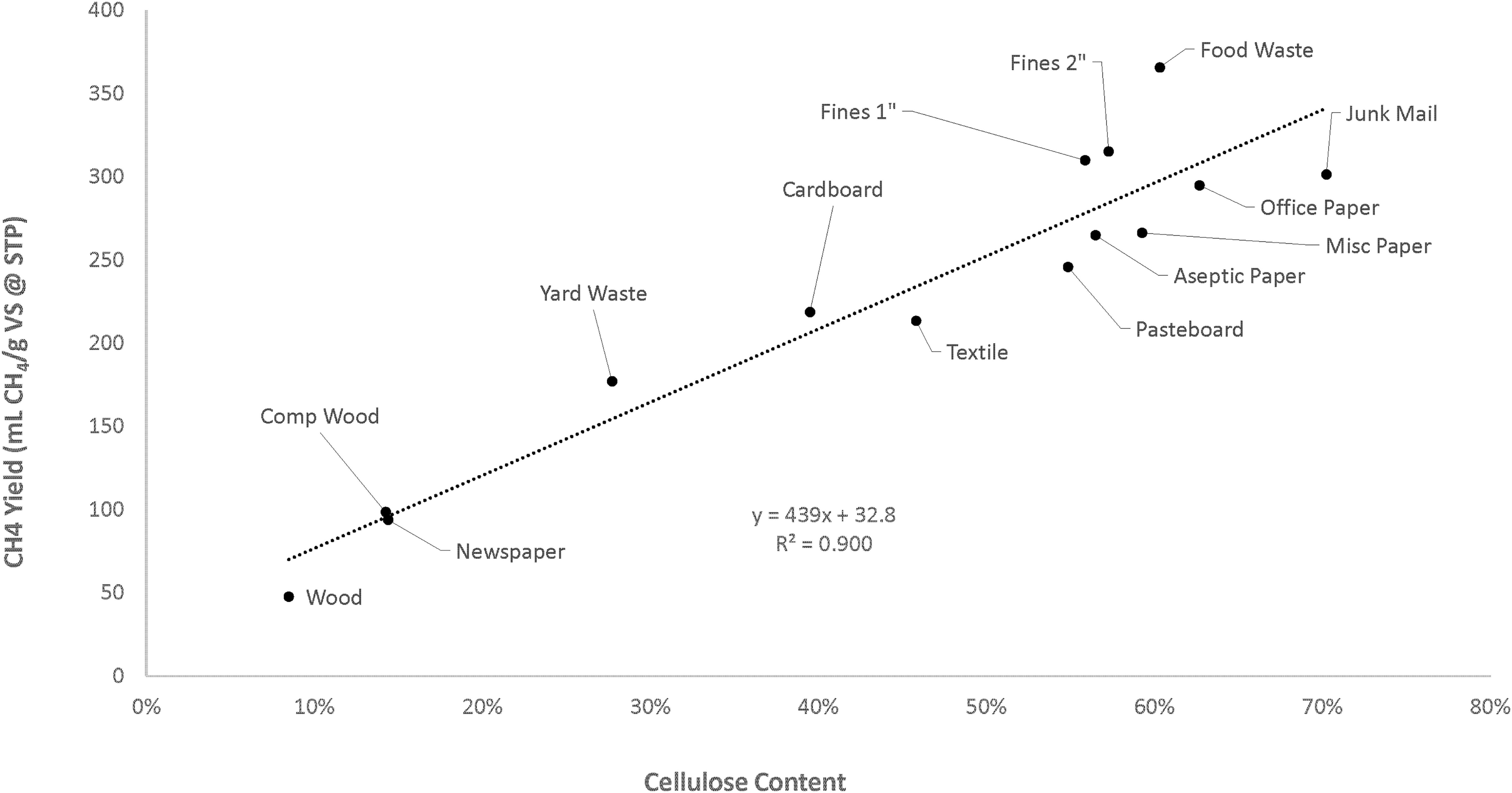
Average cellulose content of VS compared with average CH₄ yield from BMP assays by MSW fraction. Each yield value is the average of up to six samples, analyzed in triplicate. Cellulose content was determined in the same six samples through fiber analysis using Ankom 200 fiber analyzer in triplicate. BMP, biochemical methane potential.

Elemental analysis

Six samples of each organic fraction, and two samples of composite wood, were analyzed for CHONS content using an elemental microanalyzer (Elementar, Germany) at the University of California Davis Stable Isotope Laboratory. Coefficients were divided by the lowest common denominator, which was sulfur's coefficient in every sample, to simplify the chemical formula. The average chemical formula for each sample is listed in Table 3. The low sulfur content relative to C, H, and O results in large coefficients for the three major constituents. This is likely the reason that S is often left out of the formulas reported in past research (Krause et al., 2016). Comparisons to Krause et al.'s (2016) list of MSW stoichiometries show a similar trend in the fractions analyzed in this study. The H coefficient is between one to three times the magnitude of the C coefficient. The C coefficient is about one to two times the magnitude of the O coefficient and the N coefficients are one to two orders of magnitude smaller than C, H, and O.

Table 3.

Comparison of Predicted and Observed Methane Yields Based on Average Values

Fraction	Average chemical formula	Buswell prediction (mL CH₄/g VS)	Average observed yield (mL CH₄/g VS)	Ratio observed yield:Buswell prediction (“AI”), %	Lignin content (g lignin/g dry total mass), %	Anaerobic biodegradability (g C evolved to gas/g C in dry total mass), %
Cardboard	C₇₁₄H₁₁₁₃O₅₀₆N₃S	294	219	74	14	40
Newspaper	C₁₉₀₁H₂₈₀₆O₁₁₉₆N₉S	321	94	29	24	14
Office paper	C₁₅₁₅H₂₃₈₃O₁₂₅₁N₄S	255	295	116	10	56
Pasteboard	C₂₆₇₉H₄₄₇₉O₂₁₁₆N₆S	277	246	89	12	51
Junk mail	C₂₄₉₈H₃₉₂₆O₂₁₁₅N₇S	249	301	121	12	65
Aseptic paper	C₃₄₄₂H₅₂₂₁O₂₁₀₇N₈S	330	265	80	23	50
Misc. paper	C₂₂₁₂H₃₇₁₄O₁₇₀₀N₇S	277	266	96	12	52
Food and soiled paper	C₂₀₁H₃₅₆O₁₃₂N₈S	307	366	119	7	57
Yard waste	C₆₂₁H₈₃₉O₃₅₇N₁₂S	328	177	54	21	24
BFF fines <2″	C₃₉₉H₆₀₀O₂₁₈N₁₀S	342	315	92	16	49
BFF fines <1″	C₃₄₀H₄₈₃O₁₆₉N₁₆S	347	310	89	11	48
Textiles	C₂₈₃H₃₈₇O₁₆₇N₄S	315	213	68	14	44
Wood	C₃₆₈₀H₄₆₃₆O₁₉₅₄N₂₁S	343	48	14	26	8
Comp wood	C₂₈₁₆H₄₆₄₉O₁₈₆₈N₁₀₆S	306	164	53	20	11

Average stoichiometric formulas for each fraction of MSW with coefficients divided by the lowest common denominator, which was sulfur's coefficient in every sample, to simplify the chemical formula. The values listed under Ratio Observed Yield:Buswell Prediction were used as correction factors with each value serving as an AI value.

AI, average inaccuracy; BFF, biodegradable fines fraction; MSW, municipal solid waste; VS, volatile solids.

Predicted and observed methane yields

Once the empirical formulas were assembled using the elemental analysis data, methane yields were predicted using the Buswell equation. Methane yield predictions were calculated for all 80 samples and the averages for these values are listed in Table 3. Most of the observed yields listed in Table 3, measured through BMP assays, are lower than the Buswell predictions. Food and soiled paper, junk mail, and office paper produced observed yields that were larger than the Buswell predictions. Table 3 also depicts the relative magnitude of the observed yield relative to the stoichiometric yield prediction. As an example, the average observed yield of cardboard was 219 mL CH₄/g VS, which is only 74% of the 294 mL CH₄/g VS predicted by the Buswell equation. Figure 4 shows a comparison of these predicted yields and observed methane yields from this study's BMP assays. The correlation between average predicted yield and average observed yield is very low with R² = 0.098 and an increasing spread of variability with increasing predicted yield. To improve the abilities of the Buswell equation for MSW applications, individual correction factors were assigned to each fraction.

FIG. 4.

Comparison of the observed average CH₄ yields against those predicted by the Buswell equation using stoichiometries based on empirical formulas obtained from elemental analysis.

Table 3 indicates the average observed yield relative to the Buswell prediction for each of the 14 categories of MSW. These values, referred to in this study as average inaccuracy (AI), were used as a Buswell equation correction factor for each respective fraction and applied to each individual sample as shown in Equation (9). In Equation (9), AI_CF = the correction factor for average inaccuracy, B = the methane yield predicted by the Buswell equation (mL CH₄/g VS at STP), and AI_R is the average inaccuracy of the respective category of MSW—1 of the 14 categories identified in this study. $A I_{C F} = B * A I_{R}$ (9)

The results of this calculation are illustrated in Supplementary Fig. S1. The individual values of all 80 samples are shown as opposed to averages for each fraction, as a graph of average predicted yield with correction factors based on AI produces a perfect correlation. Applying the AI correction factor to each respective fraction produces a discernable trend (R² = 0.624) that is stronger than uncorrected predictions (R² = 0.098). While the average correction factor improved accuracy, additional investigation revealed another correlation.

Table 3 also shows the average lignin content of each fraction of MSW, which was calculated from using the same 80 samples analyzed for CHONS. A comparison in Supplementary Fig. S2 shows a trend of decreasing observed yields relative to predicted yields with increasing concentrations of lignin, a recalcitrant organic compound that is known to be resistant to degradation in anaerobic conditions (Bayard et al., 2018). Supplementary Fig. S2 indicates that in low-lignin fractions (12% or less) such as food waste and fines, the Buswell equation tends to underpredict methane yields. This equation was developed using agricultural products and was not necessarily intended to be used with fats and greases in food waste that is known to produce high methane yields (Buswell and Mueller, 1952). As lignin content increases over 12% the Buswell equation continues to overpredict yields in MSW fractions, the R² value (0.743) of this correlation indicates this trend could serve as both a quantitative assessment of the accuracy of stoichiometric predictions and as a method for estimating methane generation potential with empirical formulas and lignin content data.

As opposed to using one correction factor for each fraction of MSW, as practiced and displayed in Supplementary Fig. S1, a calculation was designed in which the lignin content of each individual sample was used with the equation generated with the trend line in Supplementary Fig. S2 for predicting methane yield. The original data set of 80 samples was used as a test subject. Correction factors were determined using lignin content through Ankom 200 analysis and the following Equation (10): $L C F = - 4.70 * V S_{l i g n i n} + 1.52$ (10) $L C P = B * L C F$ (11)

In Equation (10), LCF stands for lignin correction factor, which was determined using the slope of Supplementary Fig. S2 and each sample's VS_lignin value—the lignin content in the volatile solids (%). Supplementary Fig. S3 shows the average observed yield of each fraction of MSW paired with the average lignin corrected Buswell predictions, which were amended using Equation (11). In Equation (11), LCP = lignin corrected prediction (mL CH₄/g VS at STP), B = Buswell methane prediction (mL CH₄/g VS at STP), and LCF = lignin correction factor, as calculated using Equation (10). The slight increase in R² value (0.684) is a minor improvement relative to that of the AI corrected values in Supplementary Fig. S1 with R² = 0.624.

The Buswell equation is meant to apply specifically to the BF of organic materials (Achinas and Euverink, 2016). AB values listed in Table 3 were paired with Buswell predictions for methane yield and compared against observed yields in Supplementary Fig. S4. The values on the X-axis were calculated using Equation (12). $B F_{C P} = B * A B_{C F}$ (12)

In Equation (12), BF_CP = the corrected methane yield prediction using the biodegradable fraction (mL CH₄/g VS at STP), B = Buswell methane prediction (mL CH₄/g VS at STP), and AB_CF = anaerobic biodegradability correction factor, taken from values in Table 3. While a relatively strong correlation, R² = 0.866, was observed in this plot, multiplying the Buswell predictions by the AB values produced predicted yields that were lower than observed yields in all fractions of MSW. To increase the magnitude of the predicted yields, the slope intercept formula generated from Supplementary Fig. S4 was adapted to a new correction equation for estimating methane yield, shown as Equation (13). $A B F_{C P} = 1.57 * (A B * B) + 42.9$ (13)

In Equation (13), ABF_CP = the adjusted corrected methane yield prediction using the biodegradable fraction (mL CH₄/g VS at STP), AB = anaerobic biodegradability, and B = Buswell methane prediction (mL CH₄/g VS at STP). Using Equation (13) for each sample produced the average corrected methane predictions displayed in Fig. 5. The strongest correlation value of all comparisons in this study, R² = 0.922, indicates that this pairing of AB with the Buswell equation in Equation (13) should produce the most accurate methane yield predictions of all attempts in this study. This is especially true for paper products, wood, and other materials mostly derived from plant cells. Materials that deviate the most include textiles, food waste, and aseptic paper. Textiles were suspected of having minor influence by the presence of synthetic fibers that were indistinguishable in the total carbon analysis. Aseptic paper was likely to include plastic coatings in some samples, also falling subject to inorganic carbon influence in the total carbon analysis. Food waste and contaminated office paper often contained high-yielding fats and oils that were slightly underpredicted by the trendline in Fig. 5.

FIG. 5.

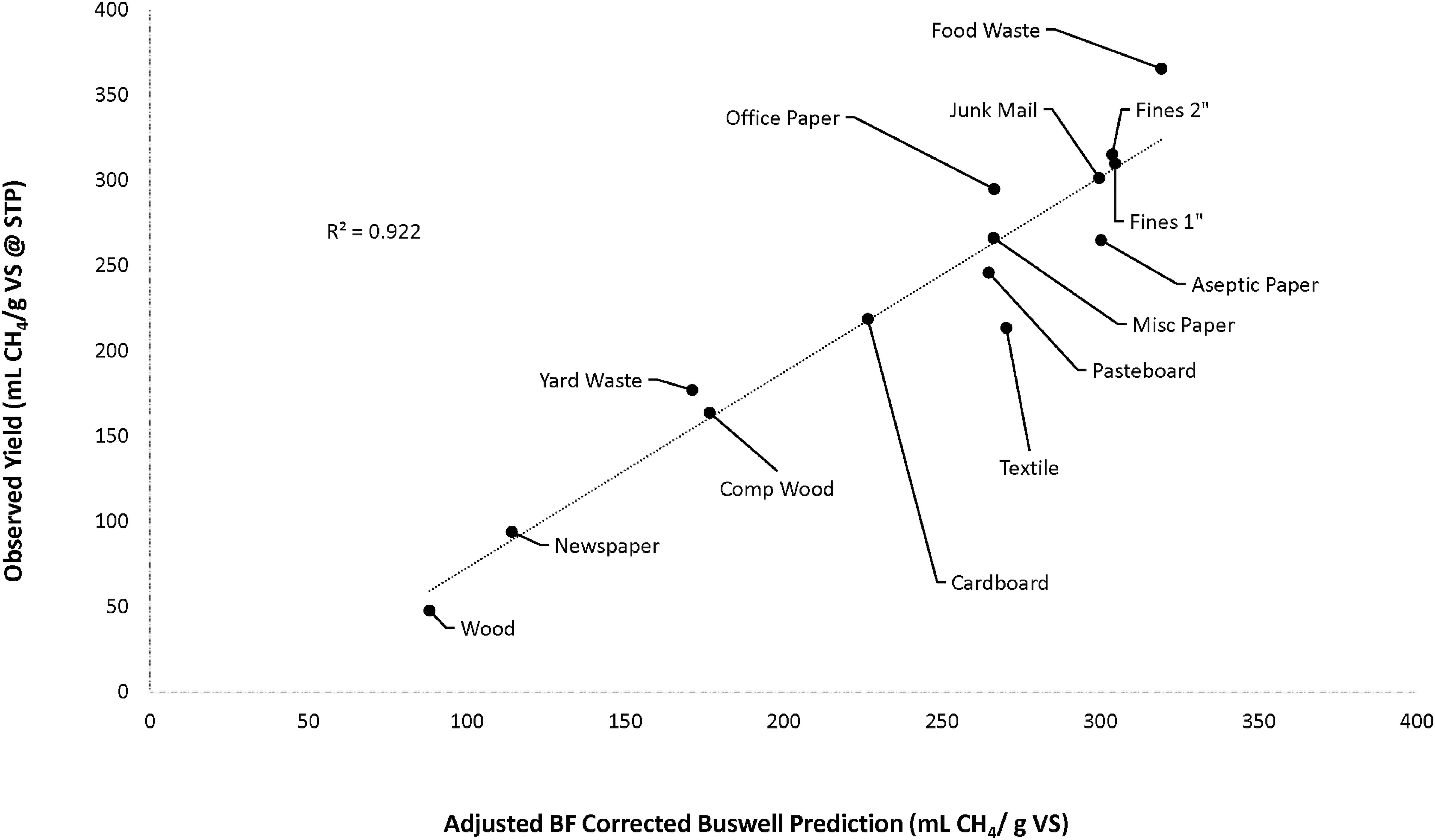
Comparison of the average observed CH₄ yield for each of the 80 samples compared to an average corrected Buswell prediction. The prediction was corrected by multiplying the stoichiometric prediction by a correction factor based on biodegradability and the linear equation displayed in Supplementary Fig. S4 [Eq. (13)].

The method of predicting yields displayed in Fig. 5 is similar to the protocol used in the IPCC's Waste Model, a tool designed to predict methane potential of MSW. The waste model incorporates a parameter termed DOC_f, which represents the fraction of anaerobically decomposable DOC in the total mass of decomposable DOC present in solid waste (Krause et al., 2016). IPCC suggests a default value of 0.5 for DOC_f in whole MSW estimates. In place of one DOC_f value to predict methane yield in whole MSW, this study proposes the use of AB values for respective fractions of MSW to more accurately predict methane yield by individual component.

Conclusions

The objective of this work was to better predict methane formation from specific categories of MSW and determine the impact of fiber content on specific MSW component biodegradability. Eighty samples of 14 types of MSW fractions were assayed through BMP, assessed for total carbon content, elemental analysis, and subjected to fiber analysis. Comparison with a correlation found by Chandler et al. (1980) in agricultural products indicated that lignin's effect on biodegradability is similar in agricultural products and biodegradable MSW components. While anthropogenic materials in MSW vary more from this and other studies' findings, the correlation should be able to accurately estimate biodegradability in solid waste.

Analyzing fiber content with a method usually applied to agricultural feed products revealed a correlation between cellulose content and methane potential, which was measured by BMP (R² = 0.900). While the material described as “cellulose” in this method may include other compounds, the method employed is highly repeatable, simpler, and much less costly than other methods that employ HPLC or other analytical equipment.

Using Buswell's equation with the elemental analysis data predicted methane yields for the MSW samples that were inconsistent with the yields observed by BMP; however, factoring in average biodegradability, determined by carbon phase conversion (solid substrate to gas byproduct), created correction factors for each of the 14 MSW categories that can be used with Equation (13) to more accurately predict methane yields instantly with stoichiometries. Comparing the average observed yields to those predicted through stoichiometry showed that MSW fractions could produce between 14% and 121% of the yield predicted by the Buswell equation. Applying the various correction factors to fractions listed in Table 3 substantially increased accuracy in yield predictions. While it may be possible to increase the complexity of methods to better predict methane yields without performing BMP assays, the use of fiber content and elemental analysis as presented in this work should provide accurate estimates without overcomplicated protocols. Sites that gather accurate waste composition data could use the research presented in this study to predict potential methane yields more accurately without implementing methane potential assays. If the lignin content or stoichiometry of the waste is determined, the ability to accurately predict methane generation can also be improved with the new methods.

Footnotes

Authors' Contributions

All authors listed made substantial contributions to the design, conception, and acquisition of data presented in this piece. All authors participated in the drafting and revisions necessary before giving final approval of the submitted version.

Acknowledgments

The authors thank the landfills, transfer stations, and waste-to-energy facilities that hosted the waste composition studies. Every student that helped analyze the many samples in numerous protocols is recognized for commitment to this multiyear project and greatly appreciated.

Author Disclosure Statement

All authors listed declare no existing or potential interests, relationships, or activities regarding this research that may have affected the outcome or reported information.

Funding Information

This research was conducted with funding from the Arcadis North America and Jacobs Technology through funding supported by the United States Environmental Protection Agency.

Supplementary Material

References

Achinas

, and Euverink

G.J.W.

(2016). Theoretical analysis of biogas potential prediction from agricultural waste. Resour. Technol. 2, 143.

ASTM D 5231-92. (2016). Standard Test Method for Determination of the Composition of Unprocessed Municipal Solid Waste 1. West Conshohocken, PA: ASTM International.

ASTM E 1196-92. (1992). Test Method for Determining the Anaerobic Biodegradation Potential of Organic Chemicals (Withdrawn 1998). West Conshohocken, PA: ASTM International.

Barlaz

M.A.

(1998). Carbon storage during biodegradation of municipal solid waste components in laboratory-scale landfills. Glob. Biogeochem. Cycles, 12, 373.

Bayard

, Benbelkacem

, Gourdon

, and Buffière

(2018). Characterization of selected municipal solid waste components to estimate their biodegradability. J. Environ. Manage. 216, 4.

Bayard

, Liu

, Benbelkacem

, Buffiere

, and Gourdon

(2016). Can biomethane potential (BMP) be predicted from other variables such as biochemical composition in lignocellulosic biomass and related organic residues?. Bioenergy Res. 9, 610.

Boyle

W.C.

(1977). Energy Recovery From Sanitary Landfills—A Review, in: Seminar Sponsored by the UN Institute for Training and Research (UNITAR) and the Ministry for Research and Technology of the Federal Republic of Germany. Göttingen: Pergamon Press.

Buffiere

, Loisel

, Bernet

, and Delgenes

J.P.

(2006). Towards new indicators for the prediction of solid waste anaerobic digestion properties. Water Sci. Technol. 53, 233.

Buswell

A.M.

, and Mueller

H.F.

(1952). Mechanism of methane fermentation. Ind. Eng. Chem. 44, 550.

10.

Cagnon

, Py

, Guillot

, Stoeckli

, and Chambat

(2009). Contributions of hemicellulose, cellulose and lignin to the mass and the porous properties of chars and steam activated carbons from various lignocellulosic precursors. Bioresour. Technol. 100, 292.

11.

Chandler

J.A.

, Jewell

W.J.

, Gossett

J.M.

, Van Soest

P.J.

, and Robertson

J.B.

(1980). Predicting methane fermentation biodegradability. Biotechnol. Bioeng. Symp. 10, 93.

12.

Chen

(2005). Biotechnology of Lignocellulose. Theory and Practice. China: Chemical Industry Press and Springer.

13.

Chen

(2014). Biological Fundamentals for the Biotechnology of Lignocellulose, in: Biotechnology of Lignocellulose: Theory and Practice. Dordrecht: Springer Netherlands.

14.

Chickering

G.W.

, Krause

M.J.

, and Townsend

T.G.

(2018). Determination of as-discarded methane potential in residential and commercial municipal solid waste. Waste Manag. 76, 82.

15.

Eleazer

W.E.

, Odle

W.S.

, Wang

Y.S.

, and Barlaz

M.A.

(1997). Biodegradability of municipal solid waste components in laboratory-scale landfills. Environ. Sci. Technol. 31, 911.

16.

Godley

, Lewin

, Graham

, Barker Oo

, and Smith

(2004). Biodegradability determination of municipal waste: An evaluation of methods. In Waste 2004 Conference on Integrated Waste Management and Pollution Control: Policy and Practice, Research and Solutions. Stratford-upon-Avon, United Kingdom, p. 40.

17.

Haug

(2018). The Practical Handbook of Compost Engineering. Boca Raton, FL: Routledge.

18.

Hettiaratchi

J.P.A.

, Jayasinghe

P.A.

, Bartholameuz

E.M.

, and Kumar

(2014). Waste degradation and gas production with enzymatic enhancement in anaerobic and aerobic landfill bioreactors. Bioresour. Technol. 159, 433.

19.

Higuchi

(2004). Microbial degradation of lignin: Role of lignin peroxidase, manganese peroxidase, and laccase. Proc. Japan Acad. Ser. B, 80, 204.

20.

Holliger

, Alves

, Andrade

, Angelidaki

, Astals

, Baier

, Bougrier

, Buffière

, Carballa

, De Wilde

, Ebertseder

, Fernández

, Ficara

, Fotidis

, Frigon

J.C.

, De Laclos

H.F.

, Ghasimi

D.S.M.

, Hack

, Hartel

, Heerenklage

, Horvath

I.S.

, Jenicek

, Koch

, Krautwald

, Lizasoain

, Liu

, Mosberger

, Nistor

, Oechsner

, Oliveira

J.V.

, Paterson

, Pauss

, Pommier

, Porqueddu

, Raposo

, Ribeiro

, Pfund

F.R.

, Strömberg

, Torrijos

, Van Eekert

, Van Lier

, Wedwitschka

, and Wierinck

(2016). Towards a standardization of biomethane potential tests. Water Sci. Technol. 74, 2515.

21.

Jayasinghe

P.A.

, Hettiaratchi

J.P.A.

, Mehrotra

A.K.

, and Kumar

(2011). Effect of enzyme additions on methane production and lignin degradation of landfilled sample of municipal solid waste. Bioresour. Technol. 102, 4633.

22.

Komilis

D.P.

, and Ham

R.K.

(2003). The effect of lignin and sugars to the aerobic decomposition of solid wastes. Waste Manag. 23, 419.

23.

Krause

M.J.

, Chickering

G.W.

, Townsend

T.G.

, and Reinhart

D.R.

(2016). Critical review of the methane generation potential of municipal solid waste. Crit. Rev. Environ. Sci. Technol. 46, 1117.

24.

Labatut

R.A.

, Angenent

L.T.

, and Scott

N.R.

(2011). Biochemical methane potential and biodegradability of complex organic substrates. Bioresour. Technol. 102, 2255.

25.

Lesteur

, Bellon-Maurel

, Gonzalez

, Latrille

, Roger

J.M.

, Junqua

, and Steyer

J.P.

(2010). Alternative methods for determining anaerobic biodegradability: A review. Process Biochem. 45, 431.

26.

Lesteur

, Latrille

, Maurel

V.B.

, Roger

J.M.

, Gonzalez

, Junqua

, and Steyer

J.P.

(2011). First step towards a fast analytical method for the determination of Biochemical Methane Potential of solid wastes by near infrared spectroscopy. Bioresour. Technol. 102, 2280.

27.

Lewis

C.G.

(2005). Linkages Among Vegetative Substrate Quality, Biomass Production, and Decomposition in Maintaining Everglades Ridge and Slough Vegetative Communities. Gainesville, FL: University of Florida.

28.

Owen

W.F.

, Stuckey

D.C.

, Healy

J.B.

, Young

L.Y.

, and McCarty

P.L.

(1979). Bioassay for monitoring biochemical methane potential and anaerobic toxicity. Water Res. 13, 485.

29.

Pipatti

, Svardal

S.P.

, Silva Alves

J.W.

, Gao

, López Cabrera

, Mareckova

, Oonk

, Scheehle

, Sharma

, and Smith

(2006). IPCC Guidelines for National Greenhouse Gas Inventories. Washington, DC: IPCC.

30.

Sánchez

(2009). Lignocellulosic residues: Biodegradation and bioconversion by fungi. Biotechnol. Adv. 27, 185.

31.

Stinson

J.A.

, and Ham

R.K.

(1995). Effect of lignin on the anaerobic decomposition of cellulose as determined through the use of a biochemical methane potential method. Environ. Sci. Technol. 29, 2305.

32.

Tchobanoglous

, Theisen

, and Vigil

(1993). Integrated solid waste management: Engineering principles and management issues. New York: McGraw-Hill.

33.

Triolo

J.M.

, Sommer

S.G.

, Møller

H.B.

, Weisbjerg

M.R.

, and Jiang

X.Y.

(2011). A new algorithm to characterize biodegradability of biomass during anaerobic digestion: Influence of lignin concentration on methane production potential. Bioresour. Technol. 102, 9395.

34.

U.S. EPA. (2020). Advancing Sustainable Materials Management: 2018 Fact Sheet. Washington, DC: U.S. EPA.

35.

Wang

(2015). Biodegradability of forest products in laboratory- and field-scale municipal solid waste (MSW) landfills. Raleigh, NC: North Carolina State University.

36.

Wang

, Padgett

J.M.

, Powell

J.S.

, and Barlaz

M.A.

(2013). Decomposition of forest products buried in landfills. Waste Manag. 33, 2267.

37.

Wang

Y.S.

, Byrd

C.S.

, and Barlaz

M.A.

(1994). Anaerobic biodegradability of cellulose and hemicellulose in excavated refuse samples using a biochemical methane potential assay. J. Ind. Microbiol. 13, 147.

Supplementary Material

Please find the following supplemental material available below.

For Open Access articles published under a Creative Commons License, all supplemental material carries the same license as the article it is associated with.

For non-Open Access articles published, all supplemental material carries a non-exclusive license, and permission requests for re-use of supplemental material or any part of supplemental material shall be sent directly to the copyright owner as specified in the copyright notice associated with the article.

0.00 MB

0.02 MB