Parallel Calculation Method for Urban Two-Dimensional Rainfall Flood Model Based on Compute Unified Device Architecture

Abstract

High-precision flood simulation can effectively give early warning or assess the corresponding risk of urban flood disaster. Recently, high-resolution terrain data have been used to completely solve the two-dimensional (2D) shallow water equations for urban flood simulations, thus improving the reliability of the results. With the development of refined terrain data, the number of calculations required for model simulations has increased significantly, and traditional parallel computing methods are becoming relatively time-consuming. This article describes the application of a parallel algorithm in the compute unified device architecture framework. A 2D hydrodynamic parallel model is established and applied to the simulation of rainfall-induced flooding in Nangang District, Harbin, China. Compared with the serial calculation method, an acceleration ratio of 42 times is obtained. Finally, the influence of different grid resolutions on the simulation accuracy and speed is discussed. The research results provide a reference for the parallel calculation of high-precision flood simulations and the formulation of simulation schemes.

Introduction

Urban flooding is a significant problem around the world. With continuing urbanization and global climate change, urban areas are more likely to suffer from sudden heavy rainfall and flooding (Fu et al., 2011; Vacondio et al., 2016). Such disasters seriously affect daily life and economic activity in cities, although timely and accurate flood forecasts can effectively reduce the effects of flood disasters on urban residents by simulating the flood process in cities. The current mainstream approaches can be divided into hydrological methods, hydraulic methods, and geographic information system (GIS)-based rapid simulation methods (Zhang and Pan, 2014). Jasper et al. (2002) coupled the atmospheric hydrologic flood runoff model and simulated it in a complex mountainous watershed.

Bates and De Roo (2000) developed a hydrodynamic model based on grating, which was successfully used to predict flood submerging norm. Nardi et al. (2019) extracted river networks from digital terrain based on GIS terrain analysis technology and further developed global flood area maps. Compared with other techniques, hydrodynamic methods can reflect the complex urban landform more accurately and provide superior information about the water depth, velocity, and inundation process over the whole area, making them more conducive to the completion of urban flood risk analysis (Teng et al., 2017).

Two-dimensional (2D) models based on the shallow water equation (SWE) are often applied for urban flood modeling using the hydrodynamic method. The results are typically used for flood risk and hazard assessment, and for the design and verification of flood control strategies (Ferrari et al., 2020). The general hydrodynamic-based urban rainfall flood model simplifies the amount of rainfall and drainage and adds it to the continuity equation (Liang and Smith, 2015).

For models that consider runoff and drainage separately, the runoff production is generally coupled with hydrological methods, and the governing equations of hydraulics and hydrological models are solved in turn (Saksena et al., 2019). Information on shared boundaries is updated and exchanged at preset computational time steps (Morita and Yen, 2002). Conventional drainage network calculation methods usually require suitable boundary conditions to calculate the transient flows in the pipeline. León et al., (2010) proposed boundary condition models for connecting and descending wells, which were coupled with Illinois transient model to simulate mixed flows in the pipeline.

Separate ordinary differential equations derived from the conservation of mass and momentum are also used to estimate the intersection flow (Borsche and Klar, 2014). Due to the different connection pipes of each node, their boundary conditions are also different, so the number of squares to be solved is also different, which ultimately leads to the complex calculation method and low efficiency.

When the hydrodynamic model is applied to actual urban flood simulations involving complex urban geometry, the resolution and quality of the topographic data will have a significant impact on the simulation results (Zoppou and Roberts, 1999; Gourbesville and Savioli, 2002). High-precision digital terrain models can be obtained based on light detection and ranging and other methods, providing the basis for high-precision numerical modeling. However, large ranges of high-resolution (10 m or less) meshes significantly increase the running time of 2D models.

With the rapid development of parallel computing technology in recent years, the computing time of high-resolution urban flood modeling is now generally acceptable. Parallel computing technologies, including the message passing interface (MPI), open multiprocessing (OpenMP), and graphics processing units (GPUs), have accelerated the research and application of large-scale flood hydrodynamic models (Judi et al., 2011; Castro et al., 2011; Kobayashi et al., 2015; García-Feal et al., 2018).

For instance, Sanders et al. (2010) proposed an MPI parallel Godunov 2D shallow water model for simulating large-scale urban dam-break floods caused by hurricane-induced storm surges. Smith et al. (2015) used GPUs to accelerate the hydrodynamic model and applied an open computing language programming framework to reproduce the floods that occurred in Carlisle, UK, in January 2005. After comparing the performance of the model on a high-specification GPU with that on a multicore central processing unit (CPU) server, their results yielded that the GPU could improve the simulation speed by more than 20 times.

Vacondio et al. (2016) developed a 2D shallow water model using the compute unified device architecture (CUDA), a GPU programming framework, to provide accurate and fast large-scale dike-break flood simulations. There have also been attempts to use multi-GPU parallelization to achieve efficient computing speeds (Sætra and Brodtkorb, 2010). These GPU acceleration models provide effective tools for large-scale high-resolution flood modeling. The results show that compared with serial codes, GPUs can significantly reduce the computation time by up to two orders of magnitude, which makes the engineering application of such models possible.

However, implementing GPU-accelerated technology to other models remains a daunting task. At present, there are also many sources of uncertainty in the storm water model that can influence the results of the model (Annis et al., 2020), such as uncertainty of rainfall, structure of the rainfall-runoff model, infiltration parameters, presoil moisture conditions, and other hydraulic factors. There are many problems in the urban stormwater model based on the hydrodynamic method, such as the integration of surface runoff, and underground pipe network drainage and the calculation speed.

It is important to study many aspects of the acceleration effect and the calculation accuracy of the model. Thus, this article describes an urban rainwater model that integrates production and confluence, resulting in enhanced simulation accuracy. Among them, the production module refers to the rainfall flow generation module, and confluence describes the confluence module after the flow generation. For lacking drainage pipe network data, the equivalent drainage method is generally adopted to simplify the complex hydrological process, but this method cannot correctly simulate runoff cycle: when the equivalent drainage efficiency is greater than the rainfall runoff, no water will be generated, and when the drainage efficiency is less than the runoff flow, flood will take place immediately. To fit the actual rainfall situation better, on the basis of equivalent drainage, the time required for flow calculation of drainage network, and the generation of excess saturated and permeable runoff are considered, the concept of aquifer is introduced.

Aquifer is specifically generalized as (1) the water storage capacity of buildings with water storage facilities, (2) the water holding capacity of soil in bare soil, roads, and vegetation areas, and (3) the water storage capacity of drainage pipes and channels. The final drainage process drains the surface and aquifer according to the drainage capacity of each area. The aquifer was introduced to connect the generating and confluence modules with the drainage modules, which corrected the calculation results of the model. At the same time, this model realizes CUDA-based parallel computing, which provides a reference for the formulation of parallel computing methods and simulation schemes for high-precision flood modeling.

Model

The establishment of an urban rainwater model includes grid construction and runoff generation, confluence, and drainage modules. The grid is constructed based on digital elevation model (DEM) data. The runoff generation module is constructed based on the rain conditions and underlying surface information, the confluence module is established using the hydrodynamic SWE, and the drainage module is developed from pipe network and drainage data. Finally, the 2D rainfall flood parallel calculation model is established based on CUDA parallel technology. Details of the modeling and simulation process are shown in Fig. 1.

FIG. 1.

CUDA-based urban rainfall flood model construction process. CUDA, compute unified device architecture.

Grid division

The watershed of the study area is obtained by DEM, and the grid boundary is determined by combining the watershed and the study boundary. As unstructured grids are more flexible than structured grids, the area of quadrilateral mesh is higher than that of triangle mesh under phase synchronous length so the number of quadrilateral mesh generated is less compared with the triangle mesh under the same resolution and the same study area. At the same time, because the friction source term adopts the calculation method of explicit format, when time discretization is carried out with the same side length, the time step of the quadrilateral is larger than that of the triangle, so as to consider the calculation cost, a quadrilateral grid is selected for the mesh division of the model.

The Gambit software is used to divide the study area into irregular quadrangular grids. Using the pipe network data, each grid cell is designed to cover at most one ground outfall. Different from the natural watershed terrain, the buildings in the city are angular, and the building grid is considered separately to describe the real terrain of the underlying surface. The grid should reflect the boundary characteristics of buildings as much as possible, and the real height of buildings should be included, so that the grid system can reflect the real underlying surface conditions, and provide basic guarantee for the accuracy of confluence calculation.

To simulate the rainfall flood process accurately, the double-layer simulation method is adopted to simulate the process of runoff generation and drainage. The overall study area is divided into two layers: the upper layer is the surface layer, which simulates the process of runoff generation and confluence, while the lower layer is the aquifer, which is included in the initial loss and drainage module of the calculation model. The upper and lower layers are divided according to the same grid resolution, so that the grids for each layer correspond to the other.

Runoff generation calculation

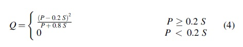
The runoff generation calculation module adopts the improved runoff curve method developed by the Soil Conservation Service (SCS) of the U.S. Department of Agriculture (Caviedes-Voullième et al., 2012). The total water balance equation in the rainfall process can be expressed as: $P = I_{a} + F + Q$ (1)

where P is the total rainfall in the basin (mm); I_a is the initial loss before runoff production (mm); F is the total loss during the runoff generation period (mm); Q is the surface runoff (mm); and S is the potential maximum retention (mm).

The two assumptions of the runoff coefficient method include: (1) the ratio of direct surface runoff to potential maximum surface runoff is equal to the ratio of infiltration to potential maximum retention; and (2) initial loss is proportional to potential maximum retention. These assumptions can be formulated as follows: $Q ∕ (P - I_{a}) = F ∕ S$ (2) $I_{a} = λ S$ (3)

where λ is the initial loss rate. Mockus (SCS, 1956) deduced that I_a = 0.2 S based on a large number of measured data and subsequently obtained the following one-parameter rainfall–runoff relationship:

where S is expressed by the dimensionless coefficient CN, namely, the curve number, and 0 ≤ CN ≤100 (Ponce et al., 1996): $S = \frac{25, 400}{C N} - 254$ (5)

The CN value for any type of land cover is determined based on the rainfall–runoff relationship, which depends on the annual maximum rainfall and the runoff generated. On this basis, the common soil moisture conditions can be summarized. The CN value of each land use mode under different hydrological soil group conditions, and the upper, lower, and middle CN values, are in accordance with the hydrological categories specified in part IV of the National Engineering Manual (neh-4) (Zia et al., 1956). According to the upper and lower limit conditions, the CN value in the model is set based on simulation tests to adjust the underground potential retention. From a comparison of the submergence process and the actual results, the underground aquifer space can then be determined.

The actual calculation of runoff generation is completed separately in each grid. After applying the unified CN value, the volume of the aquifer is obtained, and the surface water is calculated using Eq. (4), with the remainder added to the underground aquifer. When the aquifer is full of water, all rainfall is converted into surface runoff.

Confluence calculation

Confluence part adopts the 2D hydrodynamic model, simplified on the Navier–Stokes equation of 2D SWEs as flow control equations of the simulation. The explicit finite volume method is used to discretely ensure the calculation precision and speed, choose the unstructured quadrilateral grid fitting, and complex boundary for discontinuous problems adopted Roe format (Roe, 1981) approximate Riemann solution: $\frac{\partial U}{\partial t} + \nabla \cdot G = \frac{\partial U}{\partial t} + \frac{\partial E}{\partial x} + \frac{\partial F}{\partial y} = S$ (6) $\begin{matrix} U = [\begin{matrix} h \\ h u \\ h v \end{matrix}], G = (E, F), E = [\begin{matrix} h u \\ h u^{2} + \frac{g h^{2}}{2} \\ h u v \end{matrix}], \\ F = [\begin{matrix} h v \\ h u v \\ h v^{2} + \frac{g h^{2}}{2} \end{matrix}], S = [\begin{matrix} 0 \\ g h (S_{o x} + S_{f x}) \\ g h (S_{o y} + S_{f y}) \end{matrix}] \end{matrix}$

\begin{matrix} S_{o x} = - \frac{\partial Z_{b}}{\partial x}, S_{o y} = - \frac{\partial Z_{b}}{\partial y}, S_{f x} = - \frac{n^{2} u \sqrt{u^{2} + v^{2}}}{h^{4 ∕ 3}}, \\ S_{f y} = - \frac{n^{2} v \sqrt{u^{2} + v^{2}}}{h^{4 ∕ 3}} \end{matrix}

where U is the conservation vector; G is the flux vector; E is the flux in the X direction; F is the flux in the Y direction; S is the source term vector; u and v are the vertical average horizontal velocity components in the X and Y directions; g is the acceleration due to gravity; S_ox and S_oy are the source terms of the bottom slope in the X and Y directions; Z_b is the bottom elevation; S_fx and S_fy are the friction gradients in the X and Y directions; and n is the Manning coefficient.

When the finite volume method is used for numerical simulation, it is necessary to divide the computational area into a series of nonoverlapping small areas, and then select the formation mode of the control volume, conduct spatial discrete on it, and calculate the value of water flow elements in these control volumes. In this article, the central control volume method is adopted. The variables are defined in the shape center of the control body. A single grid is used as the control volume, and the control scope does not overlap each other as shown in Fig. 2.

FIG. 2.

Schematic diagram of finite volume method element.

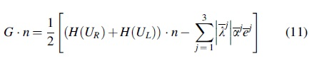
where U_i is the average value on the control volume A; $Δ S_{i}$ the area of the element; $Δ l_{i j}$ is the length of each side of the element; $G_{i j}$ is the numerical flux of each side of the element; $n_{i j}$ is the outer unit normal vector passing through the element boundary J.

For the Riemannian discontinuity problem at the interface, the physical states on both sides of the control body interface are discontinuous. The approximate Riemannian solution of Roe scheme is used to solve the normal numerical flux of the computing unit, see Toro (2013). The associated expression is as follows:

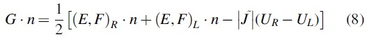
where is the average Jacobian matrix in Roe format, and U_R and U_L are conserved variables on either side of the grid cell.

The solution of the source term plays a role in stabilizing the calculation format and improving the calculation accuracy. For various complex terrain conditions encountered in reality, a reasonable solution (Toro et al., 2013) for the bottom slope source term is obtained by the characteristic decomposition of the bottom slope. A windward treatment was applied to the bottom slope term to balance the interface flux:

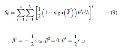
where $ẽ^{j}$ (j = 1,2,3) are the eigenvectors corresponding to the three eigenvalues of the Jacobian matrix, ${\bar{z}}_{b}$ is the average value of the left and right bottom elevations, $\bar{c}$ is the average wave velocity, $\bar{λ}$ is the right eigenvalue corresponding to the $\tilde{J}$ matrix, and sign is the sign function.

The friction source term is processed explicitly and discretely. After further discretization, the following expression is obtained:

According to eigen decomposition theory, Eq. (8) can be rearranged as follows:

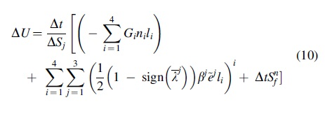
To ensure the accuracy and stability of the calculation, complex terrain requires special processing. In this article, the source term processing is performed using the bottom slope term feature method, which decomposes the source term into the bottom slope term and the friction source term, and ignores the influence of the Coriolis force. The friction source term is generally discretized in an implicit way, allowing the bottom slope stability to be considered under the abrupt flow state. The implicit discrete formula is as follows: $S_{f} = (1 - θ) S_{f}^{n} + θ S_{f}^{n + 1} = S_{f}^{n} + θ \frac{\partial S_{f}}{\partial U} \frac{\partial U}{\partial t} Δ t$ (12)

where θ is the influence weight coefficient at the next time step. When θ∈(0,1), the discrete format is semi-implicit; when θ = 0, it is fully explicit; and when θ = 1, it is fully implicit. Finally, the discrete formula is substituted into Eq. (10).

Drainage calculation

The drainage module calculates the drainage capacity of each grid, determining the overall drainage through the double-layer drainage mode. The drainage capacity of each grid depends on the distribution of the total drainage capacity and the surface outlets in the study area. The sum of the drainage capacity of all grids is the total drainage capacity of the area, and the weight of each grid is determined by the distance between the grid and the surface outlets.

When the local surface water volume is greater than the drainage capacity, the top layer has priority for drainage. When the local surface water volume is insufficient for drainage, the surface water volume is set to a minimum value, and the aquifer starts to drain. As the minimum water depth method is adopted for the dry and wet boundary treatment of the confluence part, the minimum water amount in the drainage system is set for the minimum water depth. When the water quantity is insufficient, the surface layer is set to a minimum value, and the aquifer is set to zero. The minimum water quantity Q_lim is set in the surface layer to treat the wet and dry boundary with the minimum water depth method, and to suppress any false flow at the lower water depth boundary. The specific calculation method is as follows: $\{\begin{matrix} Q_{u p}^{t + 1} = Q_{u p}^{t} - Q_{d w}, Q_{d o w n}^{t + 1} = Q_{d o w n}^{t} & Q_{u p}^{t} > Q_{d w} + Q_{lim} \\ Q_{u p}^{t + 1} = Q_{lim}, Q_{d o w n}^{t + 1} = Q_{d o w n}^{t} + Q_{u p}^{t} - Q_{d w} - Q_{lim} & Q_{u p}^{t} \leq Q_{d w} + Q_{lim}, Q_{d o w n}^{t + 1} > 0 \\ Q_{u p}^{t + 1} = Q_{lim}, Q_{d o w n}^{t + 1} = 0 & o t h e r \end{matrix}$ (13)

where Q_up is the upper water quantity, Q_down is the lower water quantity, Q_lim is the minimum water quantity, and Q_dw is the drainage quantity at the current time in the current area. The superscript t denotes the current time period, and t + 1 indicates the next time step.

Implementation of parallel method

Parallelism analysis

The purpose of parallel computing is to make full use of all computing resources and accelerate the simulation process of the model. Because the rainfall flood model is divided into several modules, it is necessary to analyze each module to determine the parallelizable area. The grid division module divides the entire area, and the grid division is calculated only once. The calculation module of this part is very efficient and the results can be saved after one implementation, without the need for parallelization. The integrated computing model needs to be rewritten in parallel, which can make full use of all computing resources and accelerate the calculation of the model.

The calculation part of the model mainly includes three modules: runoff generation, confluence, and drainage. The parallelizable analysis of each module is carried out, respectively, and the parallelizable part is rewritten by CUDA.

Time scale analysis indicates that the runoff generation and drainage models need the calculation results from the previous time step, making it difficult to achieve parallel computations on the time scale. On the spatial scale, the runoff generation module and the drainage module only need the water regime and grid information from the current surface and water-containing layer, and each grid can be divided into tasks for completion in parallel. As the confluence module is an explicit algorithm, the calculation process only needs numerical information from the adjacent grid of the current time period, so it can also be divided into different grids for parallel calculation.

Parallel algorithm based on CUDA

CUDA is a heterogeneous computing platform. Typical CUDA rewriting requires three parts: copying data from CPU memory to GPU memory, then calling kernel function to operate data stored in GPU memory, and finally returning data from GPU memory to CPU memory. The implementation of the process needs to simultaneously apply the software and hardware designed by NVIDIA and call different CUDA API functions to complete the functions of the code. Combining the CUDA acceleration technology with the parallel parts of the model, a 2D hydrodynamic rainfall flood parallel model can be realized under the CUDA infrastructure. The basic construction of the model requires the following steps:

(1) Initial environment Settings and condition input

Enter the initial boundary data in the CPU thread on the host side, call the cudaGetDeviceProperties function to obtain the GPU parameters, and clarify the details of the properties in the hardware. The grid data, rainfall sequence, and initial state are input into the model, and model parameters such as the friction coefficient, drainage coefficient, and depth of the underground aquifer are set.

(2) Identification of variable types and input of variables

The way in which the parameters are stored is the key to the construction of the CUDA model, and greatly affects the efficiency of the model. There are many constant variables, such as the minimum water depth boundary and friction coefficient in the rainfall flood model, which can be set as constant (__ constant__). All grid-related information and data, such as the water depth and velocity in the grid, are set as global variables, and space is reserved at the GPU end by calling the cudamallocmanaged function. Finally, the cudaMemcpy function is invoked to copy these global variables into the GPU memory.

(3) Task assignment and parameter design

According to the number of different cells, the calculation tasks are allocated to each thread in CUDA. The product of the number of blocks and the size of the blocks are set to be greater than the task allocation amount.

The number of simulation steps is passed into each thread through the parameters of the kernel function, and the calculation time is determined by the number of simulation steps and the individual time step. Finally, the boundary conditions of the simulation are obtained.

(4) Model simulation and result output.

By using the built-in variables of CUDA, the number of threads is calculated. This corresponds to the grid number in the rainfall flood model. Each thread corresponds to the calculation task in each grid. A single thread contains the rainfall input, initial loss calculation, confluence calculation, and drainage calculation, and then unifies the results in the current period and summarizes them in the GPU memory before the next calculation. As this summarization requires all tasks in all threads to be completed, CUDA itself does not have the function of synchronizing all blocks; this can only be completed through the implicit synchronization of the kernel function itself. Finally, a separate kernel function is opened to summarize the results and change the grid boundary type.

Through the memory copy function, the corresponding grid information is transferred from the global memory of GPU card to registers and global variables. Finally, the flux and source term calculation of the model begins, and the calculation conditions are gradually updated. The host side controls the overall calculation process. After completing the calculation of the step number, the cudaDeviceSynchronize function is called to synchronize the asynchronous operations of the CPU and GPU to ensure accurate statistics regarding the model simulation time and the accuracy of the extracted model results. Finally, the CUDA memory copy function is called to return the results from the graphics card to the host.

(5) Model optimization

The calculation process requires a large number of statistical variables or temporary variables, whereas the number of registers in the GPU card is only suitable for a small number of variables. Therefore, priority is given to the more frequently used variables, as this improves the operating efficiency of the model. In addition, the model can be further optimized by adjusting the parameters of the kernel function through debugging and running the model.

The overall realization of the model is shown in Fig. 3.

FIG. 3.

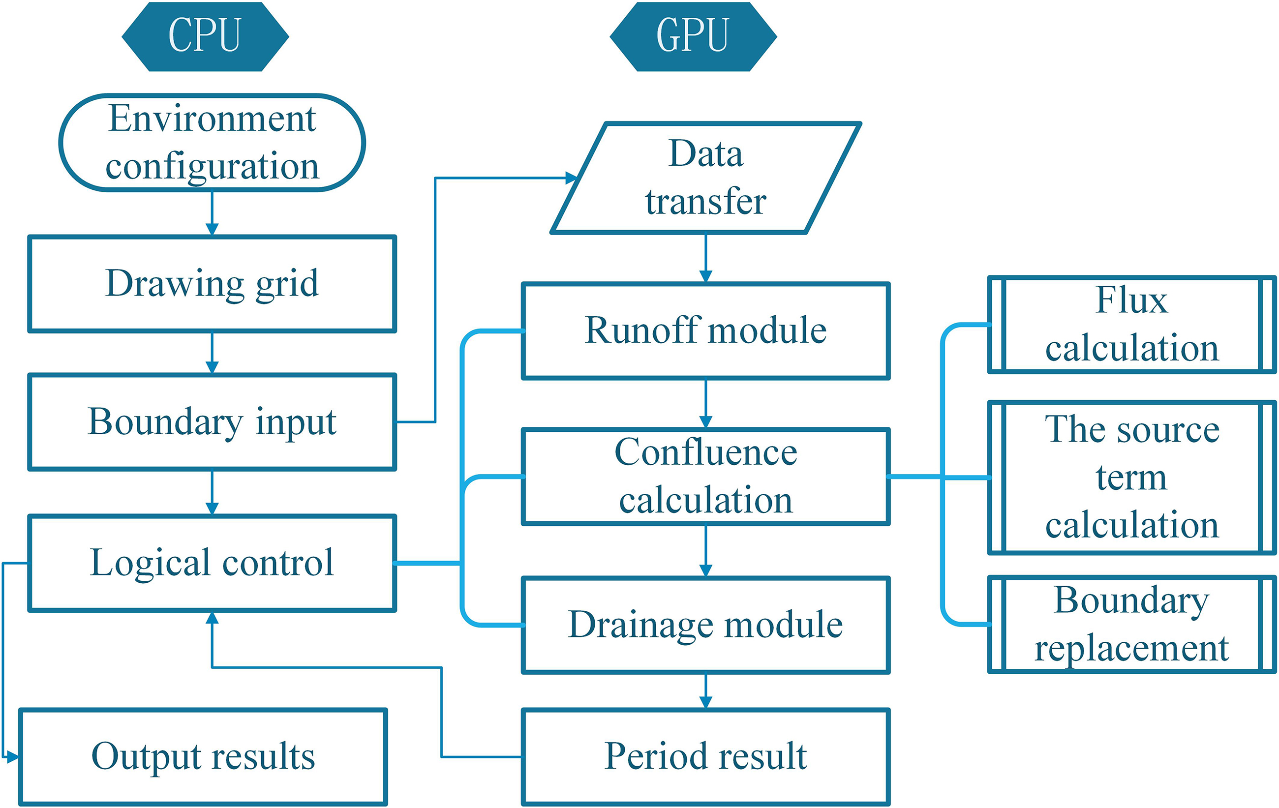
CUDA-based model parallel calculation flowchart.

Case Study: 2009 Rainstorm in Nangang District

A rainfall flood process simulation was carried out based on Nangang District, Harbin, China. The study area covers 9.1 km²; the geographical location and urban topography are shown in Fig. 4. Waterlogging disaster often occurs in Nangang District. For example, some areas of Renjie, Gogol, and Fong Xing Street are frequently inundated following prolonged rainfall. In 2009 alone, there were three flood disasters brought on by rainfall. Among them, the deepest submergence reached 40 cm and the longest single time of submergence was 2.5 h, which caused great damage to local transportation and construction facilities.

FIG. 4.

Distribution of topography and surface drainage outlets in Nangang District, Harbin.

The relevant data for the model establishment include a DEM of Nangang District with a resolution of 2 m, the 2009 rainfall data from the Harbin Rainfall Station, the Harbin City Drainage Pipeline Map, and Harbin City's 2009 medium-to-heavy rain accumulation report. The details are shown in Table 1.

Table 1.

List of Relevant Data

Data type	Type	Space-time scale
DEM	All areas of Nangang district	2 m resolution
Rainfall station	Point location and measurement information	Hour scale
Network map	Network port location
Report of heavy rain accumulation	Location and measurement information	Level of dm

The rainfall inundation process on June 4, 2009, is selected for simulation.

DEM, digital elevation model.

The rainfall inundation process on June 4, 2009, is selected for simulation. The rainfall lasted for 3 h, with 15.4 mm of rainfall in the first hour, 42.1 mm in the second hour, and 5.9 mm in the third hour. The rainfall caused different degrees of waterlogging in 11 sections of Nangang District, and the lowest inundation depth was 20 cm. Because the study area is small, it can be assumed that the rainfall is evenly distributed in time and space. The hourly rainfall in the inflow data is evenly divided according to the model time step, and the runoff yield of each period is calculated through the runoff generation module.

The drainage conditions were established according to the drainage pipe network data of Nangang District. The watershed boundary was set as a solid wall boundary, rainfall was the only water source, and the initial model water volume was set to zero. Because there are many buildings in the city, with significant topographic changes between the buildings and the ground, the stability of the model was ensured by setting the time step to 0.5 s, the minimum water depths of the dry–wet boundary to 8–10 mm, and the friction coefficient to 0.035. In the study area, the drainage capacity of the drainage pump station is 7.78 m³/s, and there are 793 surface outlets. The drainage capacity of each grid was determined by the total drainage capacity and the distribution of surface outlets.

Urban rainfall flood models of Harbin were established with average side lengths of 6, 4, and 2 m, giving corresponding grid meshes of 254,042, 559,250, and 2,104,577 cells, respectively. The models were executed in a CPU-GPU heterogeneous architecture on the Win10 operating system. The CPU was an Intel Xeon Gold 5118 and the GPU was an NVIDIA Quadro p5000.

Results

Simulation results

The rainfall lasted for 3 h, with ground overlying flow occurring after 1.5 h and reaching its maximum flow depth after 3 h. In total, the ground submergence lasted for 6.5 h. The submergence situation at a typical time is shown in Fig. 5. Our results for aquifer corresponding to maximum rainfall are graphically displayed in Fig. 6. The rainstorm caused a total submerged area of 140,800 m², with different degrees of inundation in typical flood areas, such as Renhe Street, Dacheng Street, Jianshe Street, Yinxing Street, Wenhua Street, and Lianbu Street. The average depth of submergence was 6.5 cm, with a maximum of 40.5 cm, which is basically consistent with the measured inundation in this area.

FIG. 5.

Simulation results of rainstorm inundation process in Nangang District, Harbin (2 m grid).

FIG. 6.

Aquifer results at the time of maximum rainfall (a) T = 1 h (b) T = 2 h.

In the process of confluence, the average flow velocity is only about 0.01 m/s, but high flow velocities occur in some areas (e.g., 2 m/s in Renhe Street, 0.97 m/s in Dacheng Street), which aggravate the damage caused by urban flooding.

Simulation accuracy and speed under different grid resolutions

Based on the measured submerged water depths in a typical submerged area, the simulation results under different grid resolutions were compared and analyzed. The results are presented in Table 2.

Table 2.

Comparison of Simulated and Measured Submerged Depths in Typical Urban Areas

Region	Water depth (cm)
Region	Maximum water depth in 2 m grid	Maximum water depth in 4 m grid	Maximum water depth in 6 m grid	The observations results
GuoGeLi	18.2	30	56.9	20
Renhe Street (Guangmang Street–Zhongshan Road) 1	17.9	18.5	31.9	20
Renhe Street (Guangmang Street–Zhongshan Road) 2	40.5	148.5	49.9	20
Dacheng Street (Renhe Street–Majiagou river)	36.1	31.1	146.2	20
Jianshe Street and Heyan Street corner	18	12.2	15	20
Bank Street and Jianshe Street 1	11.8	33.5	24.3	20
Bank Street and Jianshe Street 2	19.2	23.4	23.4	20
Wenhua Street 109 station	25.5	13.1	15.4	30
In front of Zhongshan garden, Lianbu Street	14.1	11.6	6.6	20
Mean absolute error (cm)	6.9	22.4	27.3
Average error (%)	34	109	134

In terms of overall accuracy, the average error on the 2-m grid is lower than that on the other two grids and the error is <1 dm. For the measurement results showing an average submergence depth of 20 cm, the average absolute error of the 4-m and 6-m grids is >20 cm. The submergence depth of each point on the 2-m grid is close to the measured value, and the accuracy at each point is better than that given by the other two schemes.

The calculation results also show that the 6-m grid gives poor submergence depths at individual points. Taking Dacheng Street (between Renhe Street and Majiagou River) as an example, an inundation depth of more than 1.4 m is generated. Because of the saturation of the drainage pipe network, the underground drainage volume is full, so the wrong submergence depths in this area are maintained for a long time. The 4-m grid produces the same erroneous results. After removing the error points, the remaining calculation results are fairly good. No unreasonable results were simulated on the 2-m grid.

From the perspective of the performance of model operation, 2-m grid needs smaller time step to ensure that the model calculated the divergence, in the process of simulation, the general performance process is more real, and calculation process smoothly. For the 6-m grid, although it can raise the corresponding time step size, due to the poor underlying surface conditions, part of the terrain connectivity is an obvious error. There are even pits made up of buildings, and as the rainfall simulation process gradually increases the amount of water eventually causes the model to collapse, where the terrain needs to be manually corrected to ensure the smooth operation of the model.

The CPU used in this article is Intel gold 5118 and the GPU is NVIDIA gv100. The calculation time and acceleration under different grid resolutions are presented in Table 3. It can be seen that the proposed model achieves an acceleration ratio of more than 42 times. Other parallel algorithms give acceleration ratios of 20.7 (OpenACC), 9.8 (OpenMP), and 5.1 (MPI algorithm) (Zhang et al., 2017). Similar CUDA framework rewriting shows that GPU can speed up computation to 15.2 times in comparison with CPU (Hou et al., 2020).

Table 3.

Simulation Time and Acceleration Ratio Under Different Grid Resolutions

Mesh accuracy	Statistical type
Mesh accuracy	Number of cells	Parallel simulation duration T_p (h)	CPU simulation time T_s (h)	Speed-up ratio
2 m	2,104,577	0.77	32.80	42.69
4 m	559,250	0.20	8.72	44.51
6 m	254,042	0.09	3.96	44.54

CPU, central processing unit.

For the 2D urban storm flood model, due to the large number of cells, OpenMP multicores need to share too much resources, so the higher number of threads cannot further improve the parallel efficiency. Compared with MPI algorithm, due to the increase in the number of cells, the increase in the number of process cores will lead to a faster increase in the cost of broadcasting, and also cannot improve the parallel efficiency. As for the OpenACC algorithm itself, due to the guide rules formulated by the top-level framework, the resource allocation in the details of the graphics card cannot be completed manually, so the improvement of efficiency only depends on the upgrade and update of the hardware itself.

All the characteristics of these three algorithms determine that they are not applicable to the 2D urban storm flood model. The CUDA acceleration algorithm corresponding to them can be very close to the application of the model and achieve good results. The acceleration effect of CUDA is much higher than that of other parallel methods. In addition, with the improved mesh accuracy and increased grid resolution, the acceleration effect of the model is enhanced, but the absolute runtime of the model only increases proportionally. Considering the operation time of the model, further improvements in accuracy would increase the runtime.

Note: Acceleration ratio calculated as $S = \frac{T_{S}}{T_{P}}$ , where T_s is the CPU serial computing time and T_p is the parallel computing time.

Comparison of models at different grid scales

In the topographic comparison map in Fig. 7, the black circle specifies the location of an abnormal inundation point. Using the topography of this point, we can directly analyze the causes of the error. The corner of Renhe Street is very narrow, and so the 2-m-wide grid gives a much better indication of the shape of the street entrance, while the 4-m grid cannot correctly describe the topography. The combination of buildings produces a relatively uneven pit around this area, and so the 6-m grid completely eliminates the existence of the channel and becomes a closed space. Therefore, for the rainfall flood results, the error with the 4-m grid is 148.5 cm in this area, while for the model with the 6-m grid, the channel is completely closed and the water is discharged through other paths, so the error in the results cannot be reflected numerically.

FIG. 7.

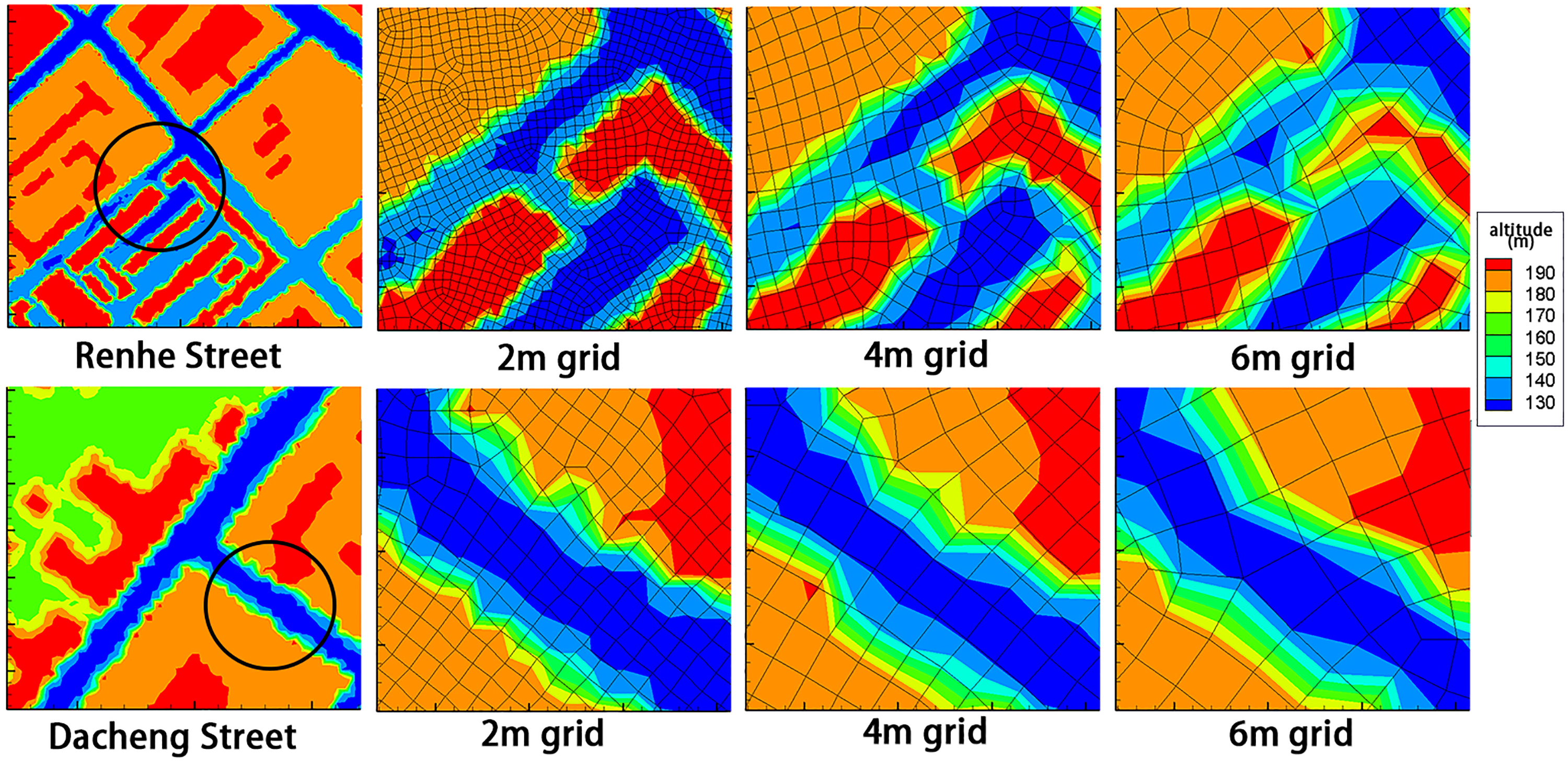
Comparison of simulation results under different grid resolutions.

Another abnormal inundation location is Dacheng Street. Because this street is wide, the 4-m grid can correctly represent the actual street, but the 6-m grid causes the terrain of the street to be too high close to the buildings. The abnormally high inundation points clearly show that the wrong terrain extends down both sides of the street. The potholes in this area eventually lead to a false submergence depth of 146.23 cm being simulated by the model with the 6-m grid.

The occurrence of abnormal inundation points reflects the impact of terrain resolution on the model simulation. Generally speaking, pothole depressions are between 2 and 7.5 cm. The 2 m grid cannot depict the detail changes of the terrain, and higher resolution DEM and grid are needed to capture such terrain details. The best model resolution needs to fully describe the underlying surface of the terrain to ensure a sufficiently high simulation accuracy.

Discussion

The number of calculations performed by the model depends on the grid scale of the model division. With a gradual decrease in the grid scale, the number of cells increases exponentially, resulting in a sharp increase in the calculation time. At the same time, a reduction in the scale of the model means that, according to the Courant–Friedrichs–Lewy condition, the time step of the model must be reduced to ensure stable simulations. For a simulation over the same period, a decrease in the time step will increase the overall number of simulation steps, which further increases the calculation time.

While the fine construction of the model more accurately reflects the actual terrain, the speed limit of the simulation means that the urban rainfall flood model cannot be completely accurate in all topographic details. To achieve the optimal balance between speed and accuracy, we need to choose the appropriate grid scale to build the model.

The results show that it takes nearly 2 days for the model to simulate the 3-h rainfall event without using parallel technology, so it cannot be applied as an actual early warning system for urban storm flooding.

When parallel methods such as OpenMP or OpenACC are used, the computing speed of the urban rainfall flood model can reach the level of real-time synchronous simulations. Using the CUDA method to accelerate the urban rainfall and flood simulation, the model can simulate 3 h of rainfall within 1 h, thus achieving the early warning function and enabling further improvements to the forecast period through subsequent optimization. Conrad (2020) used the Probabilistic Urban Flash Flood Information Nexis to consider the possible impact of a single infrastructure component on Urban Flood and use the active probability method. SWMM method was used to simulate the storm flood events, which provided important guidance and decision support.

Conclusion

This article has described the establishment of a numerical model based on CUDA for simulating urban rainfall flood processes. The SCS runoff generation module, a 2D hydrodynamic model based on an explicit finite volume method, and a comprehensive drainage model are integrated within the numerical model. The proposed model was used to simulate the rain flood inundation process in Nangang District, Harbin.

The CUDA-based model improves the computing speed by a factor of 42. Under the same computing conditions, a serial model is too time-consuming to be applied to the actual forecast and provide an early warning. Parallel methods, such as OpenMP and OpenACC, achieve real-time simulation, while the model accelerated by CUDA gives a relatively long-term prediction period.

The accuracy of the urban rainfall flood model simulation results improves as the grid resolution becomes finer, but the simulation time also increases significantly, meaning that the method could only be applied to small research areas. In contrast, an insufficient grid resolution will lead to abnormal simulations in localized areas. Therefore, it is important to select a grid resolution that can reasonably express the characteristics of the local topography and make full use of parallel computing technology.

Footnotes

Acknowledgment

The authors thank Stuart Jenkinson, PhD, from Liwen Bianji, Edanz Group, China (), for editing the English text of a draft of this article.

Author Disclosure Statement

No competing financial interests exist.

Funding Information

This study was supported by the National Natural Science Foundation of China (51979105).

References

Annis

, Karpack

, Morrison

R.R.

, and Nardi

(2022). On the influence of river Basin morphology and climate on hydrogeomorphic floodplain delineations. Adv. Water. Resour. 159, 104078.

Bates

P.D.

, and De Roo

A.P.J

. (2000). A simple raster-based model for flood inundation simulation. J. Hydrol. 236, 54–77.

Borsche

, and Klar

(2014). Flooding in urban drainage systems: Coupling hyperbolic conservation laws for sewer systems and surface flow. Int. J. Numer. Methods Fluids. 76, 789.

Castro

M.J.

, Ortega

, De la Asuncion

, Mantas

J.M.

, and Gallardo

J.M.

(2011). GPU computing for shallow water flow simulation based on finite volume schemes. Comptes Rendus Mécanique. 339, 165.

Caviedes-Voullième

, García-Navarro

, and Murillo

(2012). Influence of mesh structure on 2D full shallow water equations and SCS Curve Number simulation of rainfall/runoff events. J. Hydrol. 448, 39.

Ferrari

, Dazzi

, Vacondio

, and Mignosa

(2020). Enhancing the resilience to flooding induced by levee breaches in lowland areas: A methodology based on numerical modelling. Nat. Hazards Earth Syst. Sci. 20, 59.

, Butler

, Khu

S.T.

, and Sun

S.A.

(2011). Imprecise probabilistic evaluation of sewer flooding in urban drainage systems using random set theory. Water Resour. Res., 47, DOI: 10.1029/2009WR008944.

García-Feal

, González-Cao

, Gómez-Gesteira

, Cea

, Domínguez

J.M.

, and Formella

(2018). An accelerated tool for flood modelling based on Iber. Water. 10, 1459.

Gourbesville

, and Savioli

(2002). Urban runoff and flooding: Interests and difficulties of the 2D approach. In Proceeding of Hydroinformatics.

10.

Hou

, Kang

, Hu

, Tong

, Pan

, and Xia

(2020). A GPU-based numerical model coupling hydrodynamical and morphological processes. Int. J. Sediment Res. 35, 386.

11.

Jasper

, Gurtz

, and Lang

(2002). Advanced flood forecasting in Alpine watersheds by coupling meteorological observations and forecasts with a distributed hydrological model. J. Hydrol. 267, 40–52.

12.

Judi

D.R.

, Burian

S.J.

, and McPherson

T.N.

(2011). Two-dimensional fast-response flood modeling: Desktop parallel computing and domain tracking. J. Comput. Civ Eng. 25, 184.

13.

Kobayashi

, Kitamura

, Ando

, and Ohi

(2015). Parallel computing for high-resolution/large-scale flood simulation using the K supercomputer. Hydrol. Res. Lett. 9, 61.

14.

León

A.S.

, Liu

, Ghidaoui

M.S.

, Schmidt

A.R.

, and García

M.H.

(2010). Junction and drop-shaft boundary conditions for modeling free-surface, pressurized, and mixed free-surface pressurized transient flows. J. Hydraul. Eng. 136, 705.

15.

Liang

, and Smith

L.S.

(2015). A high-performance integrated hydrodynamic modelling system for urban flood simulations. J. Hydroinform. 17, 518.

16.

Morita

, and Yen

B.C.

(2002). Modeling of conjunctive two-dimensional surface-three-dimensional subsurface flows. J. Hydraul. Eng. 128, 184.

17.

Nardi

, Annis

, Di Baldassarre

, Vivoni

E.R.

, and Grimaldi

(2019). GFPLAIN250m, a global high-resolution dataset of Earth's floodplains. Sci. Data, 6, 1–6.

18.

Ponce

V.M.

, and Hawkins

R.H.

(1996). Runoff curve number: Has it reached maturity?. J. Hydrol. Eng. 1, 11–19.

19.

Roe

P.L.

(1981). Approximate Riemann solvers, parameter vectors, and difference schemes. J. Comput. Phys. 43, 357.

20.

Sætra

M.L.

, and Brodtkorb

A.R.

(2010). Shallow water simulations on multiple GPUs. In International Workshop on Applied Parallel Computing, Springer.

21.

Saksena

, Merwade

, and Singhofen

P.J.

(2019). Flood inundation modeling and mapping by integrating surface and subsurface hydrology with river hydrodynamics. J. Hydrol. 575, 1155.

22.

Sanders

B.F.

, Schubert

J.E.

, and Detwiler

R.L.

(2010). ParBreZo: A parallel, unstructured grid, Godunov-type, shallow-water code for high-resolution flood inundation modeling at the regional scale. Adv. Water Resour. 33, 1456.

23.

SCS (1956). National Engineering Handbook, Hydrology, Section 4, Soil Conservation Service, US Department of Agriculture, Washington, DC.

24.

Smith

L.S.

, Liang

, and Quinn

P.F.

(2015). Towards a hydrodynamic modelling framework appropriate for applications in urban flood assessment and mitigation using heterogeneous computing. Urban Water J. 12, 67–78.

25.

Teng

, Jakeman

A.J.

, Vaze

, Croke

B.F.

, Dutta

, and Kim

S.J.E.M.

(2017). Flood inundation modelling: A review of methods, recent advances and uncertainty analysis. Environ. Model. Softw. 90, 201.

26.

Toro

E.F.

(2013). Riemann Solvers and Numerical Methods for Fluid Dynamics: A Practical Introduction. Berlin, UK: Springer Science & Business Media.

27.

Vacondio

, Aureli

, Ferrari

, Mignosa

, and Dal Palu

(2016). Simulation of the January 2014 flood on the Secchia River using a fast and high-resolution 2D parallel shallow-water numerical scheme. Nat. Hazards. 80, 103.

28.

Zhang

, Li

, Jing

, Yi

, and Zhao

(2017). Comparison of three different parallel computation methods for a two-dimensional dam-break model. Math. Probl. Eng. 2017, 1970628.

29.

Zhang

, and Pan

(2014). An urban storm-inundation simulation method based on GIS. J. Hydrol. 517, 260.

30.

Zoppou

, and Roberts

(1999). Catastrophic collapse of water supply reservoirs in urban areas. J. Hydraul. Eng. 125, 686.