
Abstract
Abstract
In this study, we investigate socioeconomic inequities related to the spatial distribution and potential exposure from lead in the rapidly urbanizing region of Phoenix, AZ. We use soil lead concentrations from 200 samples collected across Phoenix as indicators of potential lead exposure, and compare them with population characteristics aggregated at the census tract level from the 2000 census, using regression and spatial autocorrelation. Percent Hispanic and percent renters are the two major regressors for lead distribution, which indicates that wealth is a weaker predictor of inequitable lead exposure than race/ethnicity and housing tenure in metropolitan Phoenix. Inequitable distribution of soil lead, likely from lead paint, reflects diminished social power, authority, and funds of neighborhoods with a high percentage of nonwhite residents living in rental housing to mitigate the potential hazard of historic lead-based paint.
Introduction
The distribution of lead in soils is often uneven, typically concentrated in poor, older neighborhoods, 9 which is a long-standing concern of environmental justice research.13–20 However, one limitation of environmental justice studies that focus on pollutants is the reliance on point source data, such as the Environmental Protection Agency's (EPA's) Toxic Release Inventory (TRI).21–25 Spatial inaccuracies in the TRI record, listing of corporate headquarter locations instead of the actual point sources of pollutant, 26 and inconsistencies in toxic release details have made it problematic to use TRI records as risk indicators. Fate and transport of lead releases are difficult to model. The EPA's Risk Screening Environmental Indicators database attempts to overcome some of these issues by modeling potential concentrations and toxicity, but is limited in its ability to measure risk. 27 Therefore, rather than relying on source data to impute the spatial distribution of lead, in this study we use soil lead concentrations from 200 random sample sites to represent a potential lead risk from anthropogenic activities. Anthropogenic lead can vary within short distances, 28 and this study is limited by the random sampling frame. However, for the purposes of this study, we assume that lead distribution obtained from these random samples is representative of the variations of lead of the greater Phoenix region. Soil is the largest sink of environmental pollutants, and also an important pathway of human lead exposure, especially for children.11,29,30 Since point sources can be extrapolated to study lead in neighborhood scales, 28 we argue that lead concentrations from random samples can depict an accurate picture of how lead in soil varies with the socioeconomic status of the local population.
Phoenix is a rapidly growing region with a population of approximately four million (U.S. Census Bureau, 2008), with 58.8% white (non-Hispanic), 31.0% Hispanic, and 4.9% African American. Prior environmental justice research in this region revealed that racial and ethnic minorities in the region bear a disproportionate burden of toxic facilities23, 31 and EPA criteria air pollutants. 32 We hypothesized that lead distribution would show the same disproportional pattern with concentrations in neighborhoods dominated by racial and ethnic minority populations.
We examine socioeconomic factors from the 2000 census, using the census tract as the unit of analysis, and compare the census data with lead concentrations from 200 samples collected across the entire metropolitan region of Phoenix. We use regression and spatial autocorrelation to check for spatial dependency with the data. In addition to modeling the relationship between race/ethnicity and lead concentrations, we investigate whether there is inequitable burden for the population most vulnerable to lead poisoning—children under the age of five. Given findings from earlier studies29, 30, 33 that link lead paint with lead soil concentrations, we also examine the relationship between housing characteristics (house age) and tenure (owners or renters) and lead concentrations.
Methods
Soil samples were taken and analyzed for lead concentrations as part of the Central Arizona Phoenix Long Term Ecological Research project's 200-point survey, where 200 sites are randomly selected across the metropolitan area of Phoenix, covering urban, agricultural, and desert land-use types 33 (Figure 1). To ensure a representative sample of the local soil, four soil cores were taken at each site from the corners of a 30×30 m square and mixed for surface (0 to 10 cm) and lower soil (10 cm to up to 30 cm) respectively. The concentrations of lead in surface soils (0–10cm) ranged from 8.2 mg kg−1 to 192.6 mg kg−1, with a median value of 22.1 mg kg−1, an average of 27.6 mg kg−1, and a standard deviation of 21.4 mg kg−1. The spatial distribution of soil lead (Figure 1) shows elevated lead concentrations in the central core of the city, as well as to the southeast. In areas dominated by desert cover, most of the samples have lead concentrations of less than 25 mg kg−1, which likely represent background lead levels of the local natural geology, given the reported continental crustal average of 17 mg kg−1. 34 Although none of the soil samples exceeds the 400 mg kg−1 level of safety standard proposed by EPA, 35 the variation of lead concentrations in different areas shows a highest lead concentration ten times more than the general desert background value, implying anthropogenic sources and disparity in lead exposure in the city. Our lead isotope study of roadside soil depth profile shows little variation going down to the depth of 25 centimeters or away from the highway from 1 to 200 meters, which negated the hypothesis of historical use of leaded gasoline. By comparing TRI data and industrial records, we also ruled out the possibility of traffic or industrial emission as the major source of lead in Phoenix, because those emissions are not enough to cause the elevated levels of lead observed in soil. By comparing lead concentrations with the building year of surrounding houses, we found that most of the high lead samples (greater than 50 mg kg−1) belong to areas with houses built before 1978, while most of the samples with a lead concentration less than 50 mg kg−1 are in areas with more recent houses, and that samples from areas with houses built before the 1940s demonstrated the highest level of lead in surface soil of all our samples. Therefore, we concluded that lead in the soil of the Phoenix Metropolitan region is more likely to have come from lead-based paint that was used before 1978 than other sources. 33
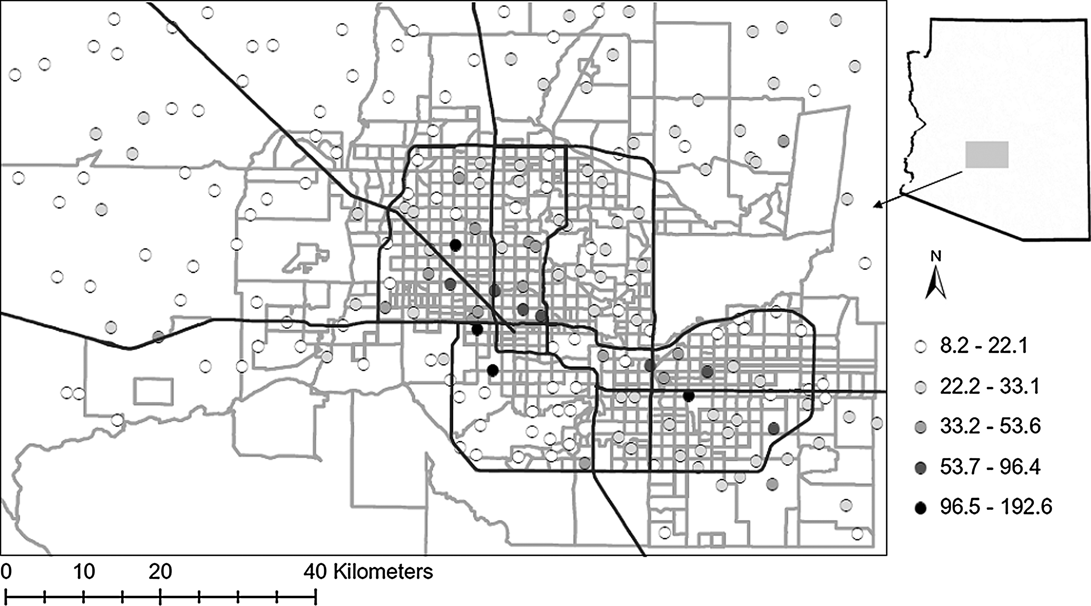
Spatial map of the surface soil lead concentrations (mg kg−1) from our study (X Zhuo. “Distributions of Toxic Elements in Urban Desert Soils” Ph.D. diss., Arizona State University, 2010) on top of census tracts outlined in light grey. The bold black lines are the major highways.
We use a geographic information system (GIS)-based analysis, and apply both linear regression and spatial autocorrelation to explore the environmental justice implications of lead variations in soil. First, we define a 1.6 km (1 mile) circular buffer around each of the 200 soil sample sites, and perform a union on each buffer with census tract polygons for the Phoenix Metropolitan Region, assuming that lead concentration from each random site is representative of the encircled area. Following the weighted average method detailed by Bolin et al., 23 and assuming within each census tract that populations are homogenously distributed, we calculate the values inside each buffer circle by summing the area weighted value of each intersecting census tract. We choose to compare socioeconomic data based on the locations of random sample sites instead of each census tract, because the latter method requires a statistical alteration of lead concentrations by kriging to predict the value inside each census tract, which introduces redundancy for spatial autocorrelation through the calculation of semivariogram and spatial lag, the key parameters for kriging and spatial autocorrelation that are based on the same spatial relations.
We selected two major factors that reflect the socioeconomic structure of the population, wealth (median household and median family income, housing tenure, and car ownership), and race (white, African American, and Hispanic), as well as vulnerability to lead exposure (children under the age of five) from the 2000 census. Income and poverty level are used to represent economic status, which is consistent with the environmental justice literature.19,20,22,23,32,36–39 Areas with a concentration of lower income households tend to be associated with more environmental hazards such as lead. In addition to income, race and ethnicity are key variables in the environmental justice literature.18,19,38 Neighborhoods dominated by racial and ethnic minorities tend to bear a disproportionate burden of environmental hazards, even controlling for income.32,40 The relatively low burden in white neighborhoods is also explained as a function of white privilege, the notion that white people can accumulate greater privileges from society by the simple act of being white, while other groups are left by default with the environmental hazards.31,41 Housing tenure is another significant factor of disproportional hazard exposure, as found by Grineski et al. 32 for air quality in Phoenix. We also used car ownership for its association with the convenience of commuting and accessibility of public facilities and benefits, 42 as well as the growing importance as an indicator of wealth in health studies.43, 44 Children under the age of six are most vulnerable to lead exposure,1, 45 but we are limited to using the census data that report children under five. We use controls (items in italics in Table 1) to distinguish each factor from the background trend of the entire population, and number of houses built before 1970 to highlight the implication of the possible source of lead-based paint. For statistical analyses, we use absolute and normalized values for population factors by census tract (Table 1).
Univariate regressions of each socioeconomic factor, control (in italics), and houses built before 1970 with lead soil contents. Data are normalized to a mean of zero and a standard deviation of 1 before regression, and standardized beta is the regression coefficient. We consider when p value is less than 0.01 (99% chance that the null hypothesis is invalid), the regression is significant. Factors that show better regression with lead than the control are highlighted in bold.
The non-normal lead concentration data were first Box-Cox transformed 46 to meet the normality assumption of a linear model, and then regressed against the socioeconomic factors calculated from above. The limitation of standard ordinary least squares regression is that it omits the spatial patterns within the sample sites. To overcome this shortcoming, spatial autocorrelation analysis36,47–51 is also applied, which adds a spatial weight of the inverse distance weighting of lead concentrations from the surrounding sample points before regression. By evaluating Moran's I, 49 if I for spatial autocorrelation is significantly greater than I0, the null hypothesis value calculated as I0=−1/(n-1), which is −0.005 here, we can reject the null hypothesis and determine that the data are spatially correlated.
Results
The Pearson correlation matrix of the socioeconomic factors (Table 2) shows severe multicollinearity inside the chosen factors, which undermines the result of a multivariate regression. Mulitcollinearity is especially strong for factors such as the absolute number of different races, households with and without cars, homeowner and renters, and children under five, which all vary in proportion to the total population inside each buffer, while factors in the form of percentages are more independent of the background population, and sheds more light on the structure of social disparity in Phoenix. For example, the percent of households without cars (Table 2) correlates positively with nonwhites (0.638 for number and 0.650 for percentage), older houses built before 1970 (0.689 for number and 0.571 for percentage), and renters (0.630 for number and 0.747 for percentage), which suggests that neighborhoods with less average economic ability to afford cars are usually areas with mostly nonwhites and renters, who usually live in older houses. In contrast, the percent of whites is the only factor that correlates positively with income (0.469 for median household income and 0.504 for median family income), and negatively with other races, renters, and households without cars, suggesting that neighborhoods with mainly whites have more socioeconomic power than those of nonwhites. Analysis of the correlation matrix (Table 2) supports Bolin et al.'s arguments regarding the strength of white privilege and race segregation in Phoenix. 31
Correlation matrix of the socioeconomic factors considered in this study. The factors used are the number of population with no car (NOCAR), the number with car (YESCAR), the number of houses (HOUSE), median household income (MHHINCOME), median family income (MFINCOME), the number of African American (AA), the number of white (WHITE), the number of Hispanic people (HISP), the number of children under the age of five (AGE5), the number of the entire population (POP), the number of homeowners (HOWNER), the number of renters (RENTER), the houses built before 1970 (HBB70), and their percentages with the prefix PCT. Correlation coefficients are in the first row, and the significance (p) is in the second row. We consider all coefficients with p<0.01 as significant. A coefficient>0.8 is strong, 0.6 to 0.8 is moderate, 0.4 to 0.6 is weak (these are all highlighted in bold), and<0.4 is a low correlation that can only be used for comparison among different factors. Factors in terms of percentage suffer less multicollinearity than numeric factors, and we star the correlations that help us explore the social disparity and its causes.
Regression and spatial autocorrelation illustrate varied potential lead exposure based on the social disparity illustrated in Table 2. The first factor in the analyses is population under five and entire population as control, which both yield significant regressions (p<0.000, meaning the null hypothesis stands less than 0.0% chance of being valid) with soil lead contents with similar standardized regression coefficients. This implies that lead exposure of children under five is similar to that of the entire population (Table 1). The less significant regression with percent under five indicates that there is little lead exposure pattern with regard to age composition of the population. Spatial autocorrelation (Table 3) shows slightly higher R2 and Moran's I with the number under five than with the entire population, and much less correlation with percent under five. Both regression and spatial autocorrelation suggest that more densely populated areas have greater potential for lead exposure, which correspond with areas that include more children under five. It is important to note that more populated areas typically have fewer whites (−0.305 for the correlation of percent whites and total population in Table 2), and these are the areas that contain more children under five and more soil lead. The correlation matrix of factors (Table 2) also shows that income correlates negatively with number of people in each buffer, so we can deduce that in poor neighborhoods where populations are usually densely settled, young children tend to be exposed to more potential lead risk than other neighborhoods.
Spatial autocorrelation results of each socioeconomic factor with control and houses built before 1970 with lead soil contents.
The second factor is race, using number of whites as control. The number of African American, Hispanic, and whites are all positive and significant (p<0.000) regressors in both regression (Table 1) and spatial autocorrelation (Table 3). However, there is little difference between results for the number of whites and African Americans in both analyses, which can be explained by the small fraction that African Americans constitute in the entire population. Hispanic population has a slightly higher R2 and regression coefficient than the control in regression (Table 1) and notably higher values in spatial autocorrelation analyses (Table 3). Thus, neighborhoods with high numbers of Hispanics are likely to have high soil lead concentrations. Comparing analysis results of percent nonwhite races with percent white (Table 1 and 3), greater differences are observed than regression by the numeric number of population. The percent of Hispanic population is a positive and significant regressor of lead (p=0.002), while percent of white is a negative and significant regressor (p=0.002).
Although income is negatively associated with percent of racial and ethnic minorities (Table 2), income is not a regressor of lead exposure. The two types of income (median family income and median household income) are not significant in the regression analysis (p>0.050 in Table 1), and they correlate negatively with lead with small values of Moran's I (-0.119 and −0.123 as in Table 3).
To examine the relationship of housing tenure and lead concentrations (Table 3), we use the number of homeowners as control, and the number and percentage of renters as regressors, and all factors yield positive and significant correlations in regression (Table 1) and spatial autocorrelation (Table 3). However, the number and percentage of renters have R2 values much greater than that of the control (homeowners) and more negative standardized regression coefficients, which means they are much better regressors of lead exposure than the control. The Moran's I for the number and percentage of renters is only slightly greater than that of the control, but renters have higher R2 than the control (Table 3). The role of housing tenure as a good indicator of lead exposure is distinct in the analyses.
The last factor is car ownership, another marker of wealth in addition to income and home ownership. We use the number and percent of household without cars as opposed to number of households with a car. Both regression and spatial autocorrelation results show that number of households without a car correlates better with lead than number of households with a car (Table 1 and 3). Percent household without a car shows less correlation than the number of households with a car and the control, but still shows significant results that more households without a car tend to have more lead exposure.
Discussion
To summarize our analyses, income and car ownership, which are indicators of wealth, are not as strong as race or housing tenure in predicting the spatial distribution of lead in the Phoenix Metropolitan Region. However, areas with high lead concentrations in soil are usually areas with mainly Hispanics and renters who have less wealth and less socioeconomic power to avoid or mitigate environmental hazards in the region. There is inequity in the distribution of potential lead exposure for minority groups and the poor compared to white populations with higher socioeconomic status.
Previous environmental justice studies have linked distributional inequities of environmental hazards to the concentration of industries in poor and nonwhite neighborhoods,20,31 the failure to protect low income and minority populations from the negative environmental consequences of urbanization, 23 and the placement of urban infrastructure such as highways, railways, and airport in those neighborhoods. 32 However, the direct link between the inequitable distribution of lead is not well-explained by the industrial geography, because industrial emissions represented by TRI are not the major source of lead in the Phoenix Metropolitan Region. 33 Nor can this inequity be attributed to transportation infrastructure, as traffic emissions do not count for the majority of the lead found in the region either. 33
Since our lead isotope study 33 points to lead-based paint as the major source of lead in Phoenix soils, we chose to investigate the association of houses with potential lead exposure (houses built before 1970s) with socioeconomic power of the population. The percent of houses built before 1970 (Table 2) shows a positive correlation with the percent of households without a car (0.571), percent Hispanics (0.497), and percent of renters (0.486), and negatively with two incomes (−0.344 and−0.289) and percent whites (-0.394). These data confirm a common pattern in North American cities, where people of lower socioeconomic status are more likely to reside in neighborhoods with old houses that contain lead-based paint. 9 The wealthy and privileged in Phoenix have historically avoided the urban center, where industries and low-income population are concentrated.
Inequitable distribution of lead among nonwhite and low-income populations may be attributed to lack of resources and social power for environmental mitigation rather than simply age of housing. In Phoenix, older neighborhoods do not necessarily correspond with higher soil lead. Regression of lead concentrations (Table 1) with number of houses built before 1970 shows only a slightly higher correlation coefficient (0.420) than with houses built in all years (0.360). The spatial autocorrelation (Table 3) with percent houses built before 1970 shows a weak association with higher soil lead concentrations (Moran's I=0.184). Thus, disparity in potential lead exposure lies mainly in the socioeconomic characteristics of population: low-income and nonwhite populations residing in older neighborhoods tend to have higher potential of lead exposure than populations living in older homes but with higher socioeconomic status. The major route of lead-based paint to the household environment is peeling of paint surfaces due to poor maintenance. 14 Populations with limited socioeconomic power may lack the funds, time, knowledge, or the authority, if renters, to prevent lead-paint contamination in and around the home.
At the same time, we also need to acknowledge that other sources of lead not examined in our study might also pose a threat to children's health in Phoenix. For example, other sources could include imported lead-contaminated candy, 52 lead-glazed ceramic ware, 53 and folk medicines. 54 Nevertheless, we hope that by measuring the levels of lead existing in the environment instead of blood lead levels, we can better illustrate the social disparity of potential lead exposure, especially when we may not fully understand all the sources of lead and their pathways to human body, which is usually the case.
Conclusion
This analysis shows a strong race-based disproportional pattern of soil lead concentrations, a relationship that is consistent with environmental justice theory. Percentage of Hispanic population—controlling for income, housing age and tenure, and spatial dependency—is the best predictor of higher soil lead concentrations in Phoenix. Since the isotope analysis shows that lead paint is the principal source of lead in this region, effective interventions to address the observed socioeconomic disparity of potential lead exposure should focus on lead-based paint mitigation. This study also demonstrates the importance of examining the environmental justice of pollution sinks rather than focusing solely on sources. In the case of potential lead exposure, environmental justice and public health efforts would benefit from cooperation on lead-based paint mitigation.