Predicting Blood-Lead Levels Among U.S. Children at the Census Tract Level

Introduction

Despite dramatic decreases in exposure, children in certain communities continue to be disproportionately harmed by lead. ¹ Identifying at-risk communities can be difficult and relies heavily on childhood blood-lead level (BLL) data; however, these data are not collected in many states, are unevenly collected in the remainder, and identify at-risk children only after they have been harmed. ² The sole national assessment of childhood lead exposure, the National Health and Nutrition Examination Survey (NHANES), is inadequate for local estimates. ³ Given the lack of BLL or tested methods to predict lead exposure, prioritization of lead poisoning prevention efforts requires support. To address this challenge, we developed a regression model to estimate childhood lead exposure in every census tract in the United States.

Our model predicts a geometric mean (GM) BLL (in micrograms of lead per deciliter of whole blood, μg/dL) for children aged 12 through 35 months as a function of predictors available for each U.S. census tract. That age range matches the NHANES data for the 1–2-year-old category; the Centers for Disease Control and Prevention (CDC) period recommends initial screening of children ⁴ and the period when most children are screened for blood lead. Unlike typically larger and more populous zipcodes, census tracts are designed to include populations with a similar socioeconomic composition. ⁵ Not surprisingly, state-level models for Rhode Island and Michigan found that a census-tract-level analysis of socioeconomic factors more strongly predicted a child's BLL than a similar zipcode analysis. ⁶

We conducted a literature review similar to that conducted by Akkus and Ozdenerol ⁷ to identify prior modeling results that suggested socioeconomic predictors for childhood BLLs. Among them were poverty, race, housing age, owner/renter status, and education. Based on the review, we evaluated the following potentially predictive socioeconomic factors related to childhood BLL available nationally at the census tract level ⁸ from the 2005–2009 American Community Survey:

1. Percentage of population below poverty line.

In addition, we considered the following potentially predictive environment factors available nationally at the census tract level from the U.S. EPA National-Scale Air Toxics Assessment (NATA) database:

10. Ambient air lead levels.

We obtained childhood BLL surveillance records from the State of Michigan (MI) Department of Community Health (n = 543,295, years 1999–2009), the Commonwealth of Massachusetts (MA) Department of Public Health (n = 833,951, years 2000–2009), and the State of Texas (TX) Department of State Health Services (n = 838,368, years 1999–2009), collected as part of their public health programs. The commonality among the states is that they screened large numbers of children. However, the states are located far from each other with commensurate differences in housing stock and environmental conditions, and they screened large numbers of children in a variety of ways. In 2000, MI and TX had a screening rate that was around the national 9.7% average screening rate whereas the MA screening rate was higher than any state and exceeded 50%. ⁹ The TX policy at the time targeted children considered high risk, whereas MA and MI widely targeted children for screening.

Each BLL record in the database corresponded to the first blood draw (venous or capillary) from a given child. ¹⁰ This enabled us to construct a representative dataset that would not be biased by oversampling children with higher levels or the inclusion of measurements after actions to reduce lead exposure. Each record was identified spatially and temporally at a sufficient level of anonymity to protect the identity of the child.

There was a unique but anonymous child ID associated with each record, and each record was assigned a geocode corresponding to the census tract where the child resided at the time of the blood draw. The actual street address was neither revealed nor needed for census-tract-level modeling. All applicable requirements of the Common Rule (40 CFR 26) were followed and the Institutional Review Boards of the MI Department of Community Health, the MA Department of Public Health, and the TX Department of State Health Services approved the human subject protections of the research report here.

For modeling purposes, we first merged the BLL data by census tract with the data for the 11 potential socioeconomic and environmental predictors. In all three states, the BLL results were reported as integer values, and because method detection limits were reported differently, we reset values lower than the detection limit to the value 1 μg/dL, thereby eliminating zeroes from the dataset and allowing the data to be log transformed. We excluded the few BLL measurements taken before 6 months of age, as prenatal exposure may be a significant source of lead exposure for such infants ¹¹ and unrelated to typical housing exposure.

We also excluded the few measurements reported as greater than 100 μg/dL due to concerns with data quality. Our goal is to predict population-level blood-lead concentrations for children who are 1 and 2 years old, but we include BLL records of children who were at least 6 months of age and a maximum of 36 months of age at the time of the blood draw so as not to exclude children who had blood-lead measurements shortly before their first birthday nor at a 3-year-old medical check-up.

In addition to the predictors available at the census tract level, the model included as covariates the season of the blood-lead sampling, ¹² whether a capillary or venous blood sample was drawn, ¹³ the age of the child, and the year of the sample. ¹⁴ Such covariates are necessary to account for long-term trends that might otherwise obscure or confound the predictive potential of publicly available data if not included in the model.

A standard log-linear regression model was fitted to the natural-log-transformed BLL records, as follows in Equation 1: \documentclass{aastex}\usepackage{amsbsy}\usepackage{amsfonts}\usepackage{amssymb}\usepackage{bm}\usepackage{mathrsfs}\usepackage{pifont}\usepackage{stmaryrd}\usepackage{textcomp}\usepackage{portland, xspace}\usepackage{amsmath, amsxtra}\usepackage{upgreek}\pagestyle{empty}\DeclareMathSizes{10}{9}{7}{6}\begin{document} \begin{align*} {y_i} = { \beta _0} + \mathop \sum \limits_j {X_{ij}}{ \beta _j} + { \epsilon _i} , \end{align*} \end{document}

where y_i represents the natural logarithm of the observed BLL for the ith observation (the measured BLL is reported as an integer number greater than or equal to one, and so the natural logarithm is well defined for all the observations); \documentclass{aastex}\usepackage{amsbsy}\usepackage{amsfonts}\usepackage{amssymb}\usepackage{bm}\usepackage{mathrsfs}\usepackage{pifont}\usepackage{stmaryrd}\usepackage{textcomp}\usepackage{portland, xspace}\usepackage{amsmath, amsxtra}\usepackage{upgreek}\pagestyle{empty}\DeclareMathSizes{10}{9}{7}{6}\begin{document} $${X_{ij}}$$ \end{document} represents the value of the jth predictor for the ith observation; \documentclass{aastex}\usepackage{amsbsy}\usepackage{amsfonts}\usepackage{amssymb}\usepackage{bm}\usepackage{mathrsfs}\usepackage{pifont}\usepackage{stmaryrd}\usepackage{textcomp}\usepackage{portland, xspace}\usepackage{amsmath, amsxtra}\usepackage{upgreek}\pagestyle{empty}\DeclareMathSizes{10}{9}{7}{6}\begin{document} $${ \beta _0}$$ \end{document} is the regression intercept; \documentclass{aastex}\usepackage{amsbsy}\usepackage{amsfonts}\usepackage{amssymb}\usepackage{bm}\usepackage{mathrsfs}\usepackage{pifont}\usepackage{stmaryrd}\usepackage{textcomp}\usepackage{portland, xspace}\usepackage{amsmath, amsxtra}\usepackage{upgreek}\pagestyle{empty}\DeclareMathSizes{10}{9}{7}{6}\begin{document} $${\beta _j}$$ \end{document} is the regression slope associated with the jth predictor; and \documentclass{aastex}\usepackage{amsbsy}\usepackage{amsfonts}\usepackage{amssymb}\usepackage{bm}\usepackage{mathrsfs}\usepackage{pifont}\usepackage{stmaryrd}\usepackage{textcomp}\usepackage{portland, xspace}\usepackage{amsmath, amsxtra}\usepackage{upgreek}\pagestyle{empty}\DeclareMathSizes{10}{9}{7}{6}\begin{document} $$\epsilon$$ \end{document} is a vector of independent and identically distributed errors after a normal distribution with mean zero and variance \documentclass{aastex}\usepackage{amsbsy}\usepackage{amsfonts}\usepackage{amssymb}\usepackage{bm}\usepackage{mathrsfs}\usepackage{pifont}\usepackage{stmaryrd}\usepackage{textcomp}\usepackage{portland, xspace}\usepackage{amsmath, amsxtra}\usepackage{upgreek}\pagestyle{empty}\DeclareMathSizes{10}{9}{7}{6}\begin{document} $$\sigma _ \epsilon^2$$ \end{document} , namely: \documentclass{aastex}\usepackage{amsbsy}\usepackage{amsfonts}\usepackage{amssymb}\usepackage{bm}\usepackage{mathrsfs}\usepackage{pifont}\usepackage{stmaryrd}\usepackage{textcomp}\usepackage{portland, xspace}\usepackage{amsmath, amsxtra}\usepackage{upgreek}\pagestyle{empty}\DeclareMathSizes{10}{9}{7}{6}\begin{document} $${ \epsilon _i} \{ \sim N \left( {0 , \ \sigma _ \epsilon ^2} \right)$$ \end{document} .

During the fitting process, significance of the predictors was judged via t-statistics for the regression parameters and the reduction in mean squared error (MSE) of the model fit when the predictor was individually added to the model. Residuals from the fitted model were examined to confirm that they appeared independent of one another and were approximately symmetrically distributed. By evaluating each of the 11 predictors one at a time, the three used in the final model were identified as providing the least MSE when predicting from one state to another and thus the best fit.

By predicting the GM BLL in the childhood population aged 12 through 35 months, one can estimate health effects such as IQ loss. ¹⁵ We also estimated the 95th percentile in the same population to describe more highly exposed children.

Model fitting based on census-tract-level predictors estimates the GM but does not directly capture the distribution of blood-lead concentrations. To capture the distribution of BLL, and thus to estimate the 95th percentile, we used an empirically calculated variance; that is, we calculated the population variance empirically as the arithmetic mean of the sample variances of the BLLs in each census tract. When validating the percentiles at the national level, we calculated the empirical variance that accounts for the difference in measurement errors between NHANES measurements and surveillance measurements.

Three analyses using Equation 1 were performed to assess the predictive ability and spatial applicability of a fitted regression model. The first analysis examined how the model functioned within MI. We split the available MI data by census tract into two subsets. The first subset, called the “training” dataset, included a random selection of two-thirds of the census tracts in the state. The second subset, called the “validation” dataset, included the remaining census tracts in the state.

We fitted the regression model to the data in the training dataset. From the fitted model, we predicted GM BLLs in the validation census tracts. For each given census tract, the socioeconomic and environmental predictor values were used in the fitted model to calculate the GM BLL that would be expected for a census tract with those predictor characteristics. We then compared the predicted BLLs with the actual surveillance data for each validation census tract to assess the accuracy of the model. The prediction errors were also examined spatially and for possible correlations with the predictors to help assess the adequacy of the model.

Because an objective of this research is to predict BLLs in states without blood-lead data, at least some of the relationships between child BLLs and the various predictors would need to be broadly applicable across spatial scales. For the second analysis, the entire dataset for MI was treated as the training dataset, and the datasets for MA and TX were treated as the validation datasets. To reduce the potential bias from TX (unlike MI and MA) targeting children considered high risk, we restricted the validation in TX to census tracts where at least 30% of the children were screened. Such a relatively high screening rate would minimize the bias from targeting for high risk.

In the absence of local surveillance data, the only quantitative option for estimating population parameters, such as GM BLL, in a community or census tract would be to use the national GM estimate from NHANES. For the third analysis, the fitted blood-lead model from MI was used at the national level to predict BLLs for every census tract in the United States. The census-tract-level predictions were then aggregated into an estimated national distribution, and the overall results were compared with measurements from NHANES.

Similar to the approach mentioned earlier, we entered U.S. census data and the other necessary predictor values into Equation 1 to calculate the expected GM BLL for each census tract in the country. Then, the weighted-GM BLL across all census tracts by NHANES wave years and child age category (i.e., 1- and 2-year-old children) was calculated, where the weighting factor was the child population in each census tract. These weighted-GM BLLs were then compared with measurements from NHANES.

For each of the three analyses, we excluded census tracts with fewer than 10 blood-lead measurements from the validation datasets as the measured population estimates would be unreliable.

Results

Modeling within Michigan

The regression model applied across census tracts in MI predicted GM BLL with an R² of 0.69. Fitting the regression model in Equation 1 with the entire MI surveillance dataset yielded regression coefficients (Table 1) that were similar to those obtained by using data from only a third of the census tracts.

OPEN IN VIEWER

Table 1.

Parameter Estimates, with Standard Errors and p-Values, for the Model Fit to the Full Michigan Dataset of Children Aged 12–35 Months Old

Coefficient	Estimate	Standard error	t value	Pr(>|t|)
Intercept	0.3514	0.0034	101.9	<10−16
Sampling test type	0.1978	0.0018	109.5	<10−16
Child age in months	0.0113	0.0001	90.7	<10−16
Year of sampling	−0.0490	0.0003	−164.4	<10−16
Month of sampling (cosine)	−0.0606	0.0012	−49.1	<10−16
Month of sampling (sine)	−0.0504	0.0012	−41.6	<10−16
Percentage of population below poverty line	0.6765	0.0075	90.1	<10−16
Percentage of pre-1960 housing	0.3999	0.0036	110.7	<10−16
Percentage of population that is non-Hispanic black	0.2277	0.0033	69.6	<10−16

The GM of BLLs in MI declined from 1999 to 2009. Childhood BLLs generally increased in the summer months and decreased in the winter months (Fig. 1). Childhood BLLs from capillary draws had a small, consistently higher level than those taken by venous draws. BLLs increased as children aged from 6 to 36 months. Using covariates substantially strengthened the predictive potential of the factors in the model.

OPEN IN VIEWER

FIG. 1.

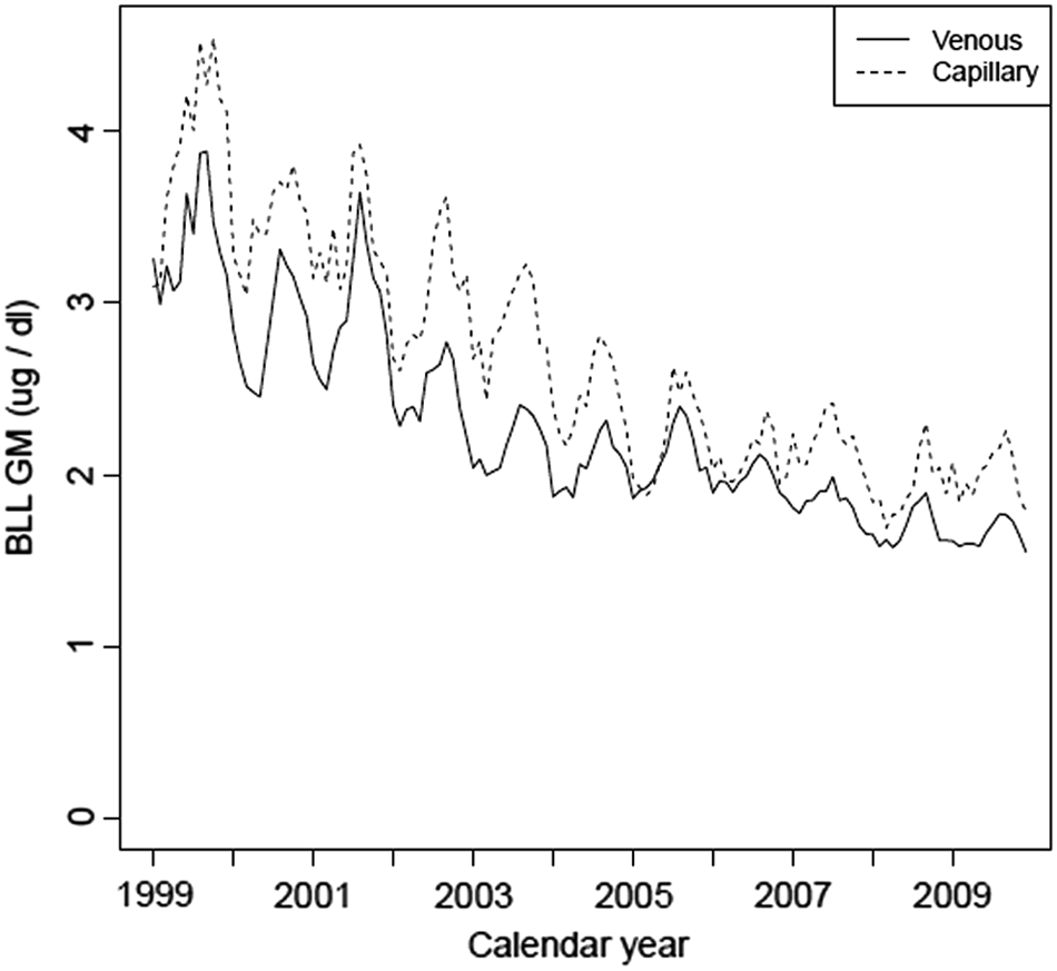
GM childhood BLL over time from 2000 to 2009 for MI. BLL, blood-lead level; GM, geometric mean; MI, Michigan.

In tandem with the adjusting covariates, the factors of “Percentage of population below poverty line” and “Percentage of pre-1960 housing” were strong predictors with highly significant (p < 0.001) coefficients. Compared with the NHANES benchmark, including the two predictors in the model reduced the MSE by 75%. The “Percentage of population that is non-Hispanic black” also had a highly significant (p < 0.001) coefficient, and adding the factor reduced the MSE by 78% compared with the NHANES benchmark while eliminating a few large outliers. Therefore, our final model included the three predictors “Percentage of population below poverty,” “Percentage pre-1960 housing,” and “Percentage of population that is non-Hispanic Black” as well as the covariates “Year of sampling,” “Month of sampling,” “Child age in months,” and “Sampling test type.” Residual analysis indicated no serious concern for conditional bias in the model predictions (e.g., no increasing or decreasing bias with increasing BLLs).

Modeling from Michigan to other states

Applying the Table 1 regression coefficients to the MA and TX data generated predicted GM BLLs for all census tracts. Figure 2 compares the predicted values against the observed GMs calculated directly from the MA and TX blood-lead surveillance data. It indicates a high degree of correlation between the predicted and observed BLLs and suggests that models that are constructed with data from one state (i.e., MI) may be generalizable to other states.

OPEN IN VIEWER

FIG. 2.

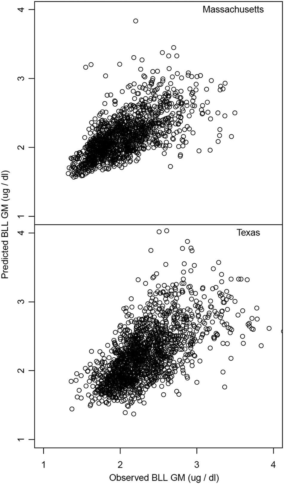
Using the MI data model, the predicted GM childhood BLL for all validation census tracts in MA plotted against observed GM childhood BLL and the predicted GM childhood BLL for all validation census tracts in TX plotted against observed GM BLL. MA, Massachusetts; TX, Texas.

Compared with the NHANES benchmark, inclusion of the housing, poverty, and non-Hispanic black predictors in the model reduced the MSE by 71% and 83% in MA and TX, respectively. The predictive model based on MI data predicted GM blood-lead concentrations in MA and TX census tracts with an R² of 0.28 and 0.20. respectively.

Though the t-statistics for “Percentage pre-1950 housing” and “Percentage pre-1960 housing” were similar, the final model included “Percentage pre-1960 housing” since it produced consistently better prediction across states. Using both housing date cutoffs did not improve predictive power, as measured by MSE, and risked instability in predicting out of state. The remaining socioeconomic and environmental predictors had far lower t-statistics that, though significant at a typical alpha level, did not consistently reduce the MSE of predictions out of state. Including them would have created more instability in predictions.

Modeling to the national level

The blood-lead regression model fitted to the MI surveillance dataset was used with predictor data for the entire United States to generate predicted GM BLLs for all census tracts in the country. These results were then combined into weighted-GM BLLs across all census tracts by year (for 1- and 2-year-old children combined), where the weighting factor in this calculation was the child population in each census tract. The weighted-GM BLLs were then compared by year with projections from NHANES (Fig. 3).

OPEN IN VIEWER

FIG. 3.

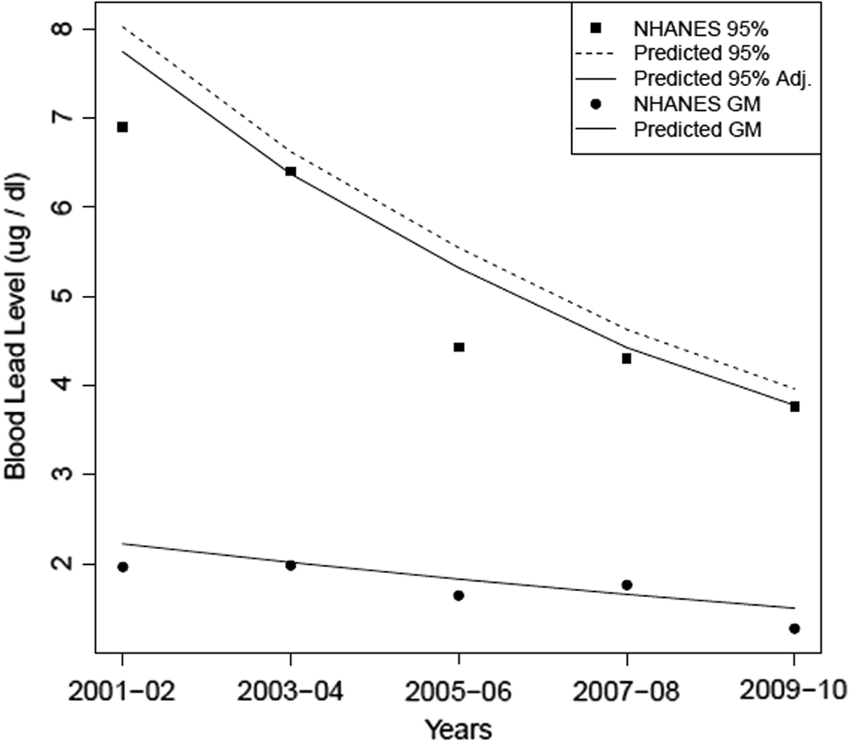
Estimated national childhood GM BLL and population 95th percentile, 2000–2009, with NHANES childhood GM and 95th percentiles shown. NHANES, National Health and Nutrition Examination Survey.

National sampling data from NHANES, including survey sampling weights, are available for five 2-year survey waves across the period of interest—those waves are 2001–2002, 2003–2004, 2005–2006, 2007–2008, and 2009–2010. These data were used to construct estimates of the national BLL distribution (GM and 95th percentiles) within each of the five survey waves. To construct predictions of the percentiles, an estimate of the variance of BLLs was estimated empirically from the MI surveillance data, and it included an adjustment to account for measurement error (estimated to be a 20% relative standard error).

Figure 3 shows the predicted percentiles with and without this variance adjustment, with the adjusted figures showing better agreement with NHANES. These results further support the idea of fitting the model in a representative state (MI) and then applying the model to other parts of the United States.

Table 2 illustrates a further level of model evaluation with the 75th, 90th, 95th, and 97.5th percentiles of the blood-lead distributions that were estimated from the predicted results and the NHANES data.

OPEN IN VIEWER

Table 2.

Predicted Blood-Lead Level in μg/dL (Michigan Model) Versus National Health and Nutrition Examination Survey Estimates, by 2-Year National Health and Nutrition Examination Survey Sampling Wave

Wave	Age	Set	GM	25%	50%	75%	90%	95%	97.5%
2001–2002	1–2	NHANES	1.98	1.30	1.90	3.10	5.50	6.90	9.40
2001–2002	1–2	Predictions	2.22	1.33	2.22	3.71	5.88	7.74	9.83
2003–2004	1–2	NHANES	1.99	1.30	1.90	2.80	4.50	6.40	8.30
2003–2004	1–2	Predictions	2.02	1.26	2.02	3.23	4.94	6.37	7.94
2005–2006	1–2	NHANES	1.65	1.13	1.62	2.35	3.33	4.43	6.46
2005–2006	1–2	Predictions	1.83	1.18	1.83	2.83	4.20	5.32	6.53
2007–2008	1–2	NHANES	1.76	1.19	1.71	2.39	3.42	4.30	6.20
2007–2008	1–2	Predictions	1.66	1.11	1.66	2.48	3.56	4.43	5.34
2009–2010	1–2	NHANES	1.27	0.86	1.20	1.83	2.65	3.76	5.78
2009–2010	1–2	Predictions	1.50	1.03	1.50	2.19	3.08	3.78	4.51

NHANES, National Health and Nutrition Examination Survey.

Similar within-state, between-state, and state to national analyses were performed by using the MA data. We found that fitting the model to the MI dataset, applying it to predictions for the entire United States agreed slightly better with the NHANES distribution, so the MI data were used in the final model.

Public health screening tool

Combining the fitted regression model with readily available American Community Survey predictor data from the U.S. Census Bureau provides predicted child BLL distributions at the census tract level for children of different ages (from 12 to 35 months of age) or for populations at different points in time (from 2000 to 2009). Such predictions provide a quantitative tool for public health and housing officials and other stakeholders promoting childhood lead poisoning prevention. In particular, these distributions can be used to assess the number of children at risk in different areas, which can then be used to help assess various intervention and resource allocation options. Figure 4 provides an example of how a map using the model of predicted GM BLLs at the census tract level for the Dallas/Ft. Worth area in Texas contrasts with a census-tract-level map of each of the socioeconomic factors incorporated into the model. Using the model, similar maps can be generated at the census tract level across the United States.

OPEN IN VIEWER

FIG. 4.

Predicted map of childhood BLLs for Dallas/Ft. Worth, TX area census tracts compared with maps of specific census-tract-level socioeconomic factors.

Discussion

If a well-developed local blood-lead surveillance program exists for the geographical area of interest, the data are useful for characterizing local conditions assuming that one accounts for year, fine-scale geography, season, and age of the child. In the absence of such a program, the results here show that it is possible to estimate childhood blood-lead concentration at the census tract level with useful predictive power.

As with summaries of local blood-lead surveillance data, these modeled screening-level estimates have uncertainty. Although these estimates will often have larger uncertainty than local surveillance data, the approach here provides an uncertainty estimate. The user can then determine whether these estimates will meet their needs, or whether follow-up surveillance is needed for census-tract-level estimates of blood-lead concentration.

Including factors for a long-term decreasing trend, a seasonal trend, and age of the child were very important for explaining the variability in the data. Each factor was highly statistically significant (p < 0.001), and not including those factors would have left substantial noise in the data. That is, knowing the age of the child, the year sampled, and the month of the year sampled allowed for an adjustment of the blood-lead concentrations that improved model estimates.

The model could not be tested at a finer resolution (e.g., census block groups) because the data for the predictive factors were not widely available at that resolution. A finer resolution may have resulted in more variability in the predictive factors and the exclusion of areas with smaller numbers in the evaluation datasets from the state surveillance registries.

Modeling childhood lead exposure in census tracts from one state (MI) to another produced R² values of 0.28–0.20 (MA and TX, respectively). Although such correlations would be very low in a physical science setting with little unit-to-unit variability and carefully controlled conditions, our setting is one of variable environmental measurements in a population of young children with widely varying activity patterns. Our modeled estimates were seen to have substantial predictive power across states and are a significant improvement over the R² value of 0 that is implied by using the NHANES national estimate for a local-level estimate. A recent study by the Washington State Department of Health/Vox ¹⁶ assigned a lead exposure risk score of 1–10 of each census tract in the United States. The study made the determination based on “Percentage of population below povery line” and “Percentage of pre-1950 housing” data in the American Community Survey and was widely publicized through a special Reuters news series. ¹⁷ In contrast to our model, the Vox maps did not evaluate the lead exposure risk score model against existing BLL surveillance data nor incorporate covariates. Our prediction evaluations included a comparison with the actual BLLs of the state with the highest rate of blood-lead screening (MA) as well as a comparison with the BLLs from the nationally representative sample of NHANES.

Using the full distribution of blood-lead concentration, rather than the percentage above certain levels, was chosen so that the results could be used in a variety of existing dose-response models relating blood-lead concentration to estimates of health impact or risk. ¹⁸ Estimates of blood-lead concentrations also can be efficiently evaluated against measurement data, where they exist; future work could develop methods for combining our predictions with local data into refined or updated estimates. Using the full distribution of BLLs facilitates the implementation of the recent CDC reference value ¹⁹ that captures all blood-lead results to focus on lead exposure at the 97.5th percentile of the population.

Questionnaires used to identify children at risk of lead exposure may be of limited value. ²⁰ However, efforts to integrate modeling results with such questionnaires to identify areas of greater risk have shown promise. ²¹ The parameter estimates in this article may provide a useful complement in areas that rely on questionnaires or incomplete lead screening databases to identify where childhood BLLs are relatively high. When measured childhood BLLs are higher than the model predicts, soil, ²² drinking water, ²³ or other potential lead exposure sources ²⁴ that exist should be investigated.

Community-scale estimates, at the census tract level, or aggregated to coarser community scales from those fine-scale estimates, have utility for local issue prioritization, for targeting areas for governmental support or enforcement targeting, and as a screening-level estimate for planning and scoping purposes for a larger risk assessment or health impact assessment. ²⁵

Our model predicts childhood BLLs in census tracts in the absence of screening data. The model results can alert public health officials to areas with potential childhood lead poisoning problems and encourage them to consider what actions to take to prevent more children from being exposed to lead.