Practical Considerations for the Interpretation of Microbial Testing Results Based on Small Numbers of Samples

Abstract

While adequate, statistically designed sampling plans should be used whenever feasible, inference about the presence of pathogens in food occasionally has to be made based on smaller numbers of samples. To help the interpretation of such results, we reviewed the impact of small sample sizes on pathogen detection and prevalence estimation. In particular, we evaluated four situations commonly encountered in practice. The first two examples evaluate the combined impact of sample size and pathogen prevalence (i.e., fraction of contaminated food items in a given lot) on pathogen detection and prevalence estimation. The latter two examples extend the previous example to consider the impact of pathogen concentration and imperfect test sensitivity. The provided examples highlight the difficulties of making inference based on small numbers of samples, and emphasize the importance of using appropriate statistical sampling designs whenever possible.

Introduction

T he presence of microorganisms in foods and food preparation environments is evaluated for a variety of reasons including pathogen detection and surveillance, outbreak investigation, or confirmation of compliance with microbiological quality requirements (ICMSF, 1986; Joint FAO/WHO Food Standards Programme, 1997; Food Standards Australia New Zealand, 2001; Joint FAO/WHO Expert Meetings on Microbiological Risk Assessment, 2012). Adequate sampling plan design is of paramount importance to assure that microbial distributions are both accurately and precisely described. Therefore, numerous guidance documents as well as statistical analysis tools have been published to support food safety sampling plan design (see, for example [ICMSF, 1986; Joint FAO/WHO Food Standards Programme, 1997; Joint FAO/WHO Expert Meetings on Microbiological Risk Assessment, 2012]). However, even though such sampling plans are widely used and represent the standard for the establishment of microbiological criteria for foods, the target sample size may not be achievable in certain situations. For example, food availability frequently limits the number of food samples available for testing in outbreak situations (Jones et al., 2004). Time and resource constraints can also limit the number of samples collected in research studies, complicating the subsequent use of such data for risk assessment or other types of inference. For example, review of the available literature on the prevalence of Listeria monocytogenes in different produce commodities revealed various studies with less than 10 available samples, at least for certain commodities (Pingulkar et al., 2001; Thunberg et al., 2002; Dhanashree et al., 2003; Johnston et al., 2006). Notably, standards to determine whether to accept a food lot traditionally also rely on sampling plans based on 10 or fewer samples (Dahms, 2004; ICMSF, 2002). Similarly, only 10 or fewer colonies are generally used when a subset of bacterial colonies isolated from a food sample is analyzed for further isolate identification (FDA, 2011a). Therefore, inference sometimes has to be made based on data from a small number of samples, even though adequate, statistically justified numbers of samples should be obtained whenever feasible.

It has been shown that humans tend to be inherently insensitive to sample size considerations when interpreting sampling results—a heuristic commonly referred to as “representativeness” in the area of cognitive psychology (Tversky and Kahneman, 2008). As a result, the degree of confidence in small samples tends to be overestimated, especially if sampling variability is not explicitly evaluated (Tversky and Kahneman, 2008). This underestimation of sampling variability can pose considerable practical problems. For example, if only small numbers of samples are tested, the presence of pathogens is likely to be missed (ICMSF, 1986). The failure to detect the pathogen in any of the selected samples may be interpreted erroneously as the absence of pathogens in the target population if the limited ability of the analysis to detect the pathogen is not considered. Routine testing of small numbers of samples may repeatedly fail to detect the presence of a pathogen or specific pathogen strain, especially if the prevalence is low. In such cases, the sudden detection of the pathogen or strain following repeated false-negative (i.e., failure to detect the pathogen even though it is present) testing results may be interpreted erroneously as a recent introduction of the pathogen or strain, or as the emergence of a new (e.g., multidrug-resistant) strain. The interpretation of data based on small numbers of samples is therefore complicated and requires careful consideration of sampling probabilities.

To provide some practical observations that may be helpful for the interpretation of results based on a small number of samples, we analyzed the impact of small sample sizes on pathogen detection and prevalence estimation. We evaluated four situations commonly encountered in practice, with the first two examples evaluating the combined impact of sample size (i.e., number of samples) and pathogen prevalence (i.e., fraction of food items that are contaminated) on pathogen detection and prevalence estimation, and the latter two examples extending the previous example to consider the impact of pathogen concentration (i.e., average concentration of pathogen cells) and imperfect test sensitivity (i.e., ability of the test to correctly classify samples that contain at least one pathogen cell). The statistical foundations for this work are well known (see, for example [ICMSF, 1986; Vose, 2000; ICMSF, 2002; Gardner, 2004; ILSI, 2010; FDA, 2011b). However, the practical implications of these statistical relationships are frequently not considered in practice. As will be discussed in the final part of this article, the statistical evaluations provided below make several simplifying assumptions regarding test performance, pathogen distribution in the food item, and testing scheme that are unlikely to be fully met in practice. Therefore, as discussed below, in reality the performance of food testing schemes is likely to be lower than presented here (ILSI, 2010).

Statistical Evaluations of Common Applications for Microbial Testing Data

In the following two sections, we will evaluate the combined impact of pathogen prevalence (i.e., fraction of food items that are contaminated in a lot) and sample size (i.e., number of samples) on pathogen detection or prevalence estimation, respectively.

Probability of detection as a function of sample size and pathogen prevalence

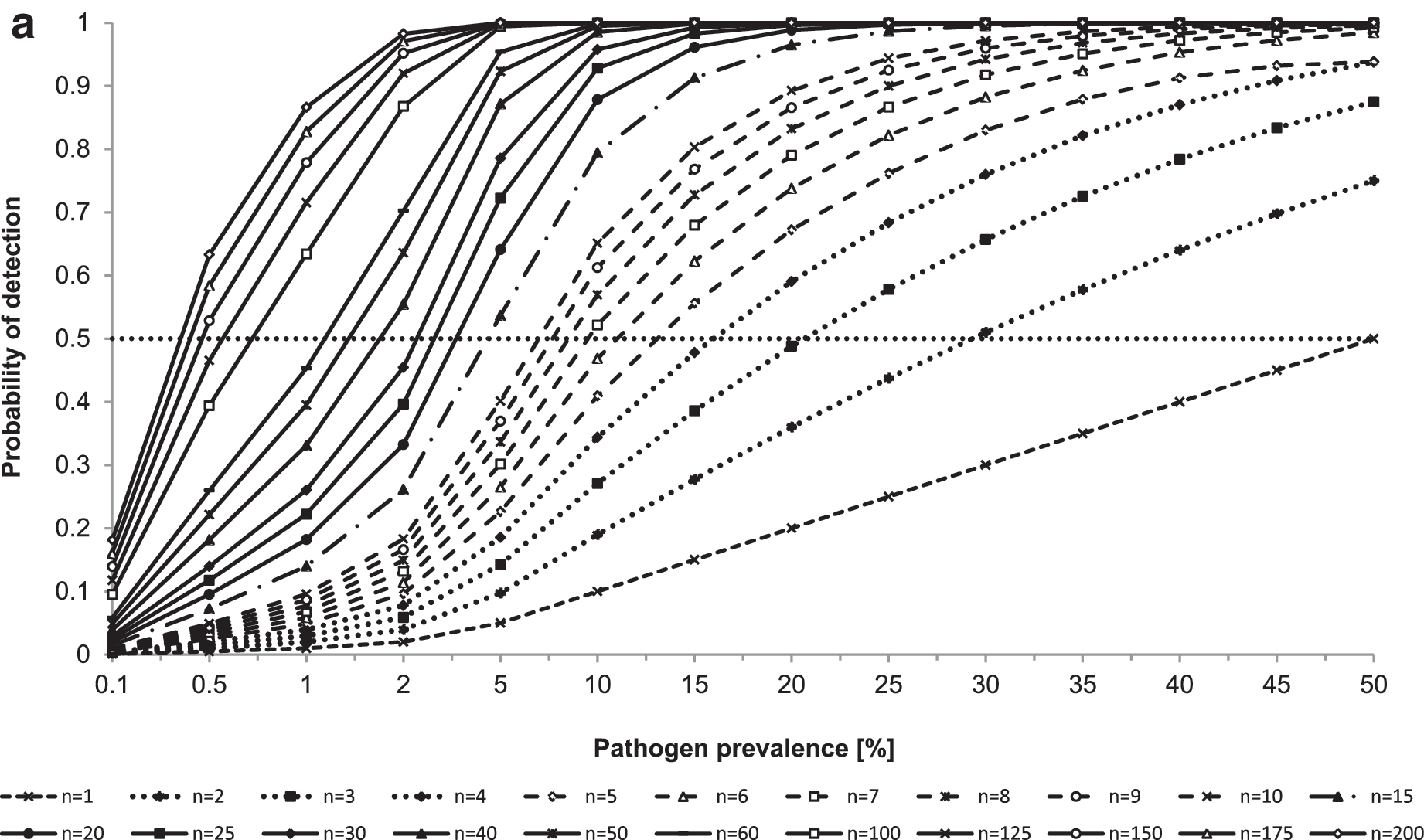
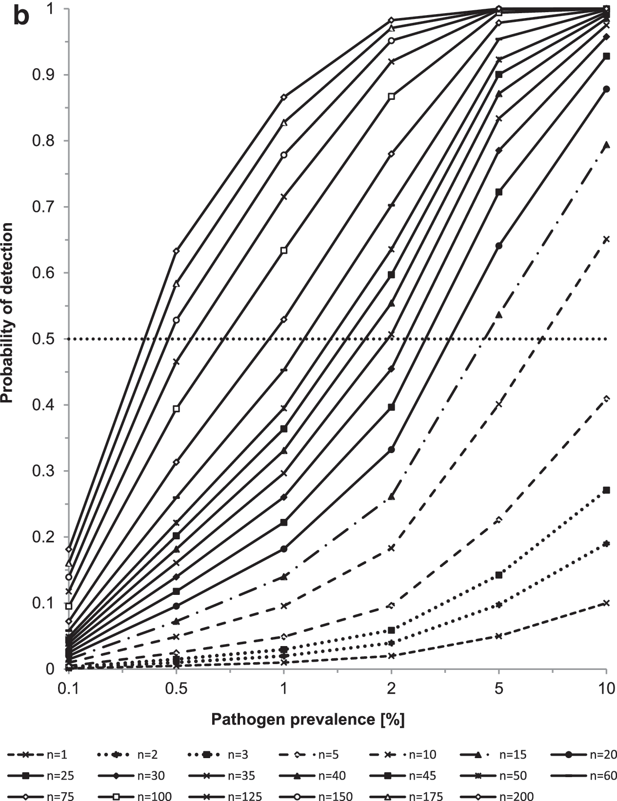
Consider one lot, consisting of numerous food items, is tested to determine whether pathogens are present in the lot. Only a subset of n food items is selected for testing. Assume a perfect test, so that all contaminated food items (i.e., defined in this scenario as containing at least one bacterial cell) will be classified correctly as pathogen positive, and all uncontaminated food items (i.e., defined in this scenario as containing zero bacterial cells) will be classified correctly as pathogen negative (Fig. 1, scenario 1). Assume further that each food item has the same probability p of being contaminated and that the sample of size n is collected from among all available food items in the lot in such a way that every possible combination of n food items has an equal chance of being selected (i.e., simple random sample). Finally, assume that only a relatively small fraction of all food items in the lot is tested, so that each item would be unlikely to be selected more than once (i.e., sampling probabilities with and without replacement are comparable). Our objective is to determine whether the lot is contaminated. The probability of detecting k=0 positive samples in the sample of size n can be evaluated from the binomial distribution. For this special case, the density simplifies to Prob (k=0)=(1−p)ⁿ, where p is the pathogen prevalence (i.e., fraction of contaminated food items), n equals the total number of collected samples, and k equals the number of positive samples. The probability of detecting at least one positive sample is then given by Prob (k>0)=1−(1−p)ⁿ.

FIG. 1.

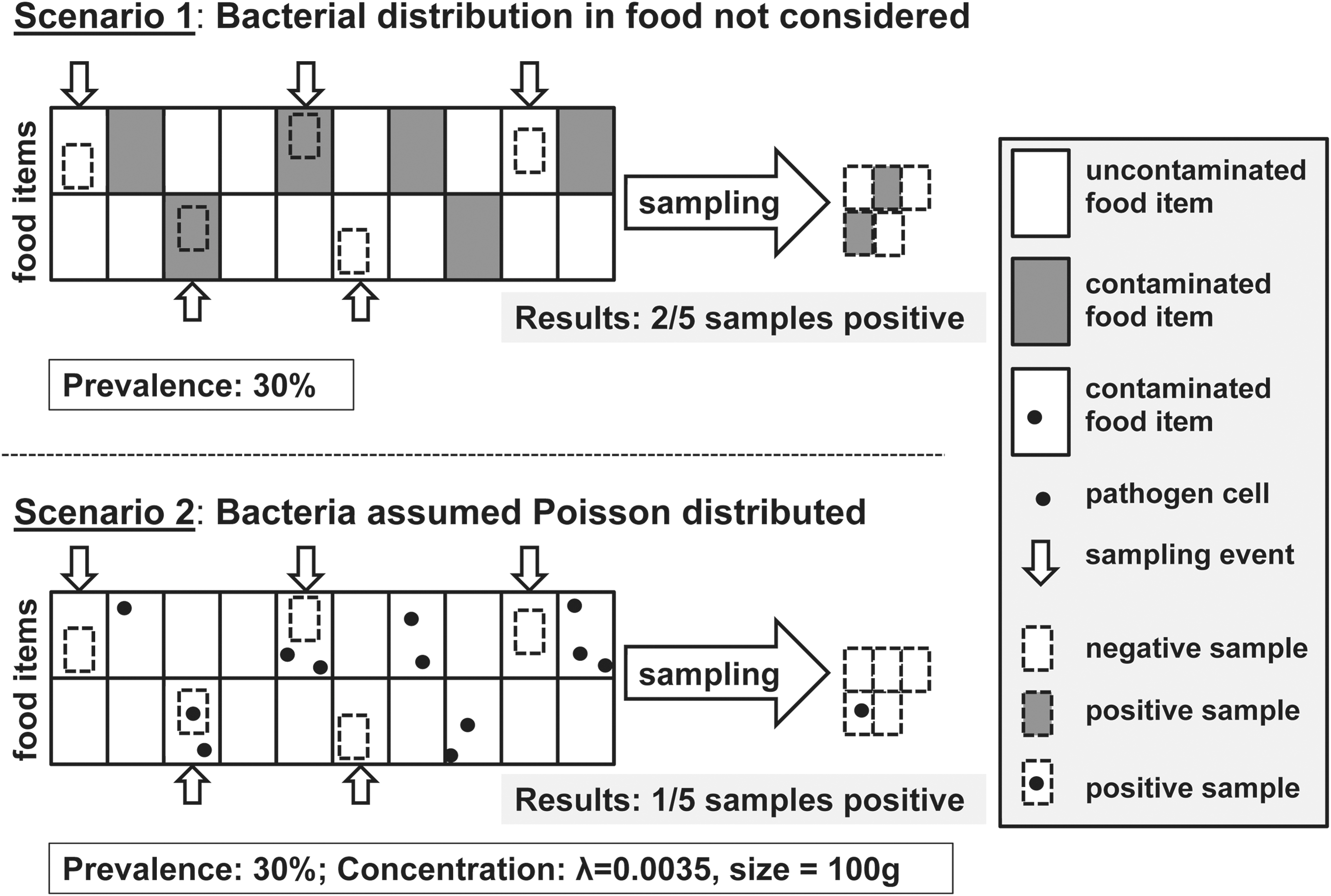
Comparison between scenarios in which every sample of a contaminated food item is assumed to be test-positive and the number of contaminated food items is assumed to be binomially distributed (i.e., Scenario 1), and scenarios where the concentration of pathogens in contaminated food items is assumed to be Poisson distributed and therefore not every sample from a contaminated food item is assumed to be test-positive (i.e., Scenario 2).

Figures 2a and b illustrate the impact of the number of collected samples and of the pathogen prevalence on the probability of detection (i.e., the probability of detecting the pathogen in at least one sample). If the number of samples is small—for example, if six samples are collected—even pathogens that are present in 10% of food items are more likely to be missed than detected (i.e., probability of detection of 0.47). In fact, 22 samples are needed to detect pathogens present in 10% of food items with 0.9 probability. If the pathogen is only present in 5% of food items, 45 samples are needed to detect the pathogen in at least one sample with 0.9 probability, and if the pathogen is only present in 1% of food items, 230 samples are needed. Therefore, very large sample sizes are needed to determine the likely absence of a pathogen of interest. If a relatively small number of samples fail to detect the presence of a pathogen of interest, these results need to be interpreted carefully, in light of the limited statistical power to detect pathogens present at a low prevalence.

FIG. 2.

a: Probability of detecting at least one positive sample when testing a lot, as a function of the total number of samples (for n=1 to n=200) and pathogen prevalence (for prevalence between 0.01 and 0.5); a horizontal line indicates a probability of 0.5, signifying a probability of detection equal to that of flipping a (fair) coin. b: Probability of detecting at least one positive sample when testing a lot, as a function of the total number of samples (for n=1 to n=200) and pathogen prevalence (for prevalence between 0.01 and 0.1); a horizontal line indicates a probability of 0.5, signifying a probability of detection equal to that of flipping a (fair) coin.

Prevalence estimation as a function of pathogen prevalence and sample size

Assume the same assumptions apply as described above. Our objective is now to evaluate the pathogen prevalence (i.e., fraction of food items in a given lot that are contaminated). To evaluate the degree of confidence that can be placed in prevalence estimates generated based on a small number of samples, we calculated confidence intervals around the prevalence estimates. Because of the small sample size and relatively low prevalence, commonly used normal approximations for confidence intervals around binomial fractions are likely inappropriate here (Vose, 2000). We estimated exact confidence intervals, based on the method first described by Clopper and Pearson (Clopper and Pearson, 1934), even though the resulting confidence limits are conservative in that they tend to be wider than their nominal coverage (Angus and Schafer, 1984).

Figure 3 shows the exact confidence intervals surrounding various observed prevalence estimates for a total of n=10 samples. The confidence intervals are very wide, reflecting the low degree of confidence that should be placed in prevalence estimates generated based on small numbers of samples. The 95% confidence interval for a sample size of 10 and an observed prevalence of five positive samples ranges from 19% to 81%, whereas the 95% confidence interval for an observed prevalence of one positive sample ranges from 0.2% to 44%. In either case, prevalence estimates based on a sample of size 10 are likely highly imprecise. Figure 4 provides confidence intervals for observed prevalence estimates of 0, 0.1, 0.2, 0.3, 0.4, and 0.5 and sample sizes ranging from n=10 to n=50. Figure 4 illustrates that large sample sizes are necessary to derive reliable prevalence estimates. If, on the contrary, judgments need to be based on small numbers of samples, it may be preferable to express the estimated prevalence in the form of a fraction (where the sample size is given in the denominator of the fraction) instead of decimals to emphasize the small number of samples on which the results are based, and to provide the associated confidence interval to emphasize the limited degree of confidence that should be placed on these estimates.

FIG. 3.

Ninety-five percent exact binomial confidence intervals (Clopper and Person, 1934) surrounding observed prevalence estimates, based on a sample of size n=10. Crosses denote observed prevalence estimates, while horizontal lines indicated 95% confidence intervals surrounding the observed prevalence estimates.

FIG. 4.

Ninety-five percent confidence intervals for an observed prevalence of 0, 0.1, 0.2, 0.3, 0.4, and 0.5, as a function of sample size (for a sample size of n=10, 20, 30, 40, and 50). Solid lines indicate observed prevalence estimates, while dotted lines indicated 95% confidence intervals surrounding the observed prevalence estimates.

In the following two sections, we will expand the previous considerations by relaxing the assumption of a “perfect test.” Specifically, we will explore the impact of sample size, pathogen concentration, and test sensitivity (i.e., probability of correctly detecting the pathogen in a sample if it is present) on detection probabilities.

Probability of detection as a function of pathogen concentration, amount of food sampled, and sample size

So far, we assumed that any given sample collected from a contaminated food item will contain at least one cell of the pathogen of interest (Fig. 1, scenario 1). However, even if a pathogen is assumed to be homogeneously distributed in a given food, by chance none of the bacterial cells may be included in a sample of a given size if the pathogen concentration in the food is low or if the physical sample size is small (Fig. 1, scenario 2). We extend the previous considerations to such situations where not every sample of a contaminated food item (i.e., containing at least one pathogen cell) may contain the pathogen. Our objective is again to determine whether a given lot is contaminated. Assume the same assumptions hold as before, but consider that pathogens are present in a given contaminated lot with some mean concentration λ (e.g., expressed as colony-forming units (CFU)/mL or CFU/g). Each sample is of some physical size s (e.g., expressed in grams or milliliters). Assume that the number of bacteria in a lot is homogeneously distributed (i.e., Poisson distributed with parameter λ). The probability of detecting the pathogen in k=0 samples taken from n food items that are part of the contaminated lot is now given by the Poisson distribution. We have Prob (k=0)=(e ^−λsn) and the probability of detecting the pathogen in at least one sample of size s equals Prob (k>0)=1−(e ^−λsn). Note that the probability of detection is determined by the product λ * s * n, so that any equivalent product of these three parameters (e.g., n=100, s=25 g, λ=0.001 CFU/g and n=10, s=10 g, λ=0.025 CFU/g) will yield exactly the same probability.

Figure 5 shows the probability of pathogen detection for such sampling, for samples of physical size 10 g and 25 g, for bacterial concentrations of 0.01–0.3 CFU/g, and for sample sizes of n=1 to n=30. Results for 25-g samples are shown in black and results for 10 g samples are shown in gray. As expected, the sample size n, the physical size of the sample s, and the pathogen concentration in the food item λ are major determinants of the probability of detection. Notably, for samples of 10 g and a pathogen concentration of 0.01 CFU/g, seven samples are needed for the pathogen to be as likely detected as missed (i.e., probability of detection of 0.5). Even in a sample of 25 g, a pathogen present at a concentration of 0.01 CFU/g is missed about eight times out of 10, and at least three samples are needed in this case to achieve a detection probability above 0.5. Therefore, if pathogen concentrations are low, even under the assumption of homogeneous distribution of pathogens in the food, large sample sizes are needed and the physical amount of food sampled needs to be relatively large to avoid missing the presence of pathogens in the food samples.

FIG. 5.

Probability of detection (i.e., detecting at least one positive sample) based on samples of 10 g (gray dashed lines) or 25 g (black solid lines) obtained from a contaminated lot, as a function of the total number of collected samples (for n=1 to n=30) and the average pathogen concentration in the food items (for concentrations between 0.01 colony-forming units [CFU]/g and 0.3 CFU/g). For combinations of physical size of the sample and pathogen prevalence that generate identical results (e.g., 25 g and 0.04 CFU/g; 10 g and 0.1 CFU/g) only one representative graph is displayed (see text for details).

Probability of detection as a function of sample size and sensitivity of the test

Until now, we assumed that the diagnostic test is perfectly sensitive and specific, so that samples containing at least one pathogen cell would be correctly classified as pathogen positive, and samples with zero pathogen cells would be correctly classified as pathogen negative. While it may be reasonable to assume that microbiological tests, especially those based on culture methods, are highly specific (i.e., yield no false-positive results), the sensitivity (i.e., probability of detecting the pathogen if it is present in the sample) of the microbiological test is unlikely to be perfect (Gardner, 2004). To extend the previous considerations to tests with imperfect diagnostic sensitivity, assume that all other conditions apply as before, but that the probability of the test detecting the pathogen (if it is truly present in a specific sample of a contaminated food item) is given by se, the sensitivity of the test, and assume further that se is constant for a given diagnostic test being applied to detect a specific pathogen in a given type of contaminated food item, regardless of the bacterial concentration in the sample. Our objective is again to determine whether a given lot is contaminated. The probability of obtaining a positive test result now depends on two probabilities: (1) the probability of at least one bacterial cell being present in a given sample, and (2) se, the probability of the test detecting the presence of the pathogen if at least one pathogen cell is present in a given sample. Using the same rationale as above, the probability of b=0 bacterial cells being present in a given sample of size s is given by Prob (b=0)=(e^−λs ). Se denotes the conditional probability of the pathogen being detected, given that it is present in the sample, so that Prob (detection | b>0)=se, and Prob (no detection | b>0)=(1−se). Therefore, the probability of detecting k=0 positive samples among the n tests is given by Prob (k=0)=((e ^−λs)+(1−e ^−λs) * (1−se))ⁿ, and the probability of detecting at least one positive sample is then given by Prob (k>0)=1−((e ^−λs)+(1−e ^−λs) * (1−se))ⁿ. Figure 6 shows the probability of detecting the pathogen in at least one 25-g sample from a lot contaminated with an average concentration of 0.03 CFU/g, as a function of test sensitivity and number of collected samples. Figure 6 clearly shows that, as test sensitivity decreases, the number of samples needed to detect the presence of pathogens increases, especially if pathogen concentrations are low.

FIG. 6.

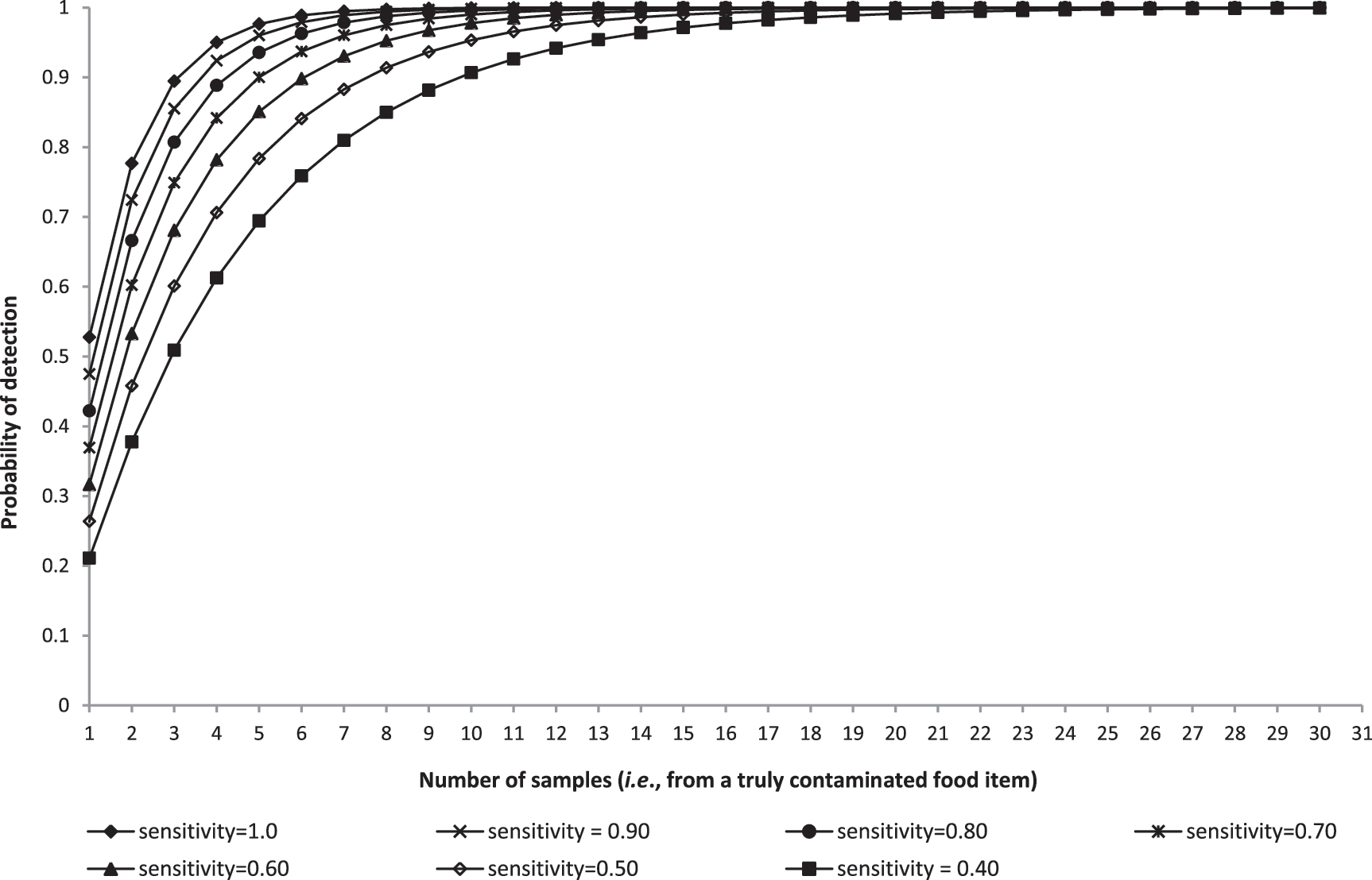
Probability of detection (i.e., detecting at least one positive sample) based on samples of 25 g obtained from a contaminated lot with average pathogen concentration of 0.03 colony-forming units/g, as a function of the total number of collected samples (for n=1 to n=30) and diagnostic test sensitivity (with diagnostic sensitivity ranging from 1.0 to 0.4).

Discussion of Additional Considerations for Sampling Under Practical Conditions

The statistical evaluations provided here make numerous simplifying assumptions that are rarely fully met in practice. One assumption we already discussed concerns perfect test specificity. For a variety of reasons, diagnostic tests are generally neither perfectly sensitive nor specific (Greiner and Gardner, 2000). However, even if diagnostic tests are never truly perfectly specific, the specificity of microbiological test methods is generally high and the probability of detecting false-positive results in a relatively small number of samples is therefore very low (Gardner, 2004), leading us to the simplifying assumption of perfect test specificity because our analysis focuses on small sample sizes. Yet, in practice, false-negative as well as false-positive test results may under certain circumstances complicate the interpretation of microbial testing data (Greiner and Gardner, 2000; FDA, 2007). The predictive values of a test (i.e., the fraction of true-positive or true-negative test results among positive or negative test results, respectively) need to be considered in the evaluation of testing results (see, for instance, [Gardner, 2004] for a comprehensive review of this important but complex topic, which is beyond the scope of this article).

Sensitivity and specificity as defined here (also commonly referred to as “diagnostic sensitivity” and “diagnostic specificity”) apply at the sample level, and measure the probability of correctly classifying samples that do (i.e., sensitivity) or do not (i.e., specificity) contain the pathogen. We assumed independence between diagnostic sensitivity and the number of pathogen cells present in a given sample, an assumption that may not be true in practice. “Analytical sensitivity” measures the ability of a test to consistently detect low numbers of bacteria, and is often expressed as the “limit of detection,” the lowest concentration of a pathogen that can be consistently (i.e., typically in ≥95% of samples) detected (Saah and Hoover, 1997; FDA, 2011b). The limit of detection of a particular test method, determined by the amount of food sampled and the minimum number of pathogen cells that can be detected in a sample by a given test, also necessarily needs to be considered in the interpretation of sampling data (Hardin, 2011).

We here considered testing of 10-g and 25-g food samples because these represent commonly used sampling amounts for the microbial testing of foods (see, for instance, (New South Wales Food Authority, 2008; EFSA, 2010; FDA, 2011). However, samples of other size may clearly also be chosen (Gombas et al., 2003; Dahms, 2004; FDA, 2011a), and the results presented here can easily be extrapolated to other sampling amounts and bacterial concentrations. However, despite the assumptions made here, pathogens are generally not homogeneously distributed in food (Jongenburger et al., 2011; ILSI, 2010; Jongenburger et al., 2012a; Jongenburger et al., 2012b), and this heterogeneity necessarily reduces the probability of detection for a pathogen (Jongenburger et al., 2012b); therefore, especially if bacterial concentrations are low, the probability of capturing at least one pathogen cell in a sample from a contaminated lot is likely markedly lower than assumed here (Hardin, 2011).

We considered a situation where all food items were contaminated with the same probability. In the real world, contamination may be limited to parts of a lot (ICMSF, 1986; Jongenburger, 2012b). Therefore, food items within a lot or across lots often do not all have the same probability of being contaminated. Moreover, we considered a simple random sample where each combination of food items had the same probability of being selected. In practice, however, it is often unfeasible for practical and economic reasons to sample food items with truly equal probability of selection (ICMSF, 1986), potentially leading to more complex sampling situations (Levy, 2005). Moreover, our examples only considered presence/absence testing, even though pathogen enumeration is an important part of many microbial evaluations of foods, and generally associated with even greater uncertainties (FDA, 2011). In reality, inference based on small numbers of samples is therefore more complicated and less certain than presented here.

The results presented here undoubtedly emphasize the difficulty of making inference based on small numbers of samples. A positive test result obtained with a small or very small sample size suggests, but does not necessarily indicate, a highly contaminated lot. Our results also indicate that, if additional tests are to be performed after an initial positive test result, retesting of the initial positive sample or additional tests on the isolated pathogen, if available, may be preferable to the collection of additional samples from the same food lot because the probability of detection in the additional samples may be low if bacterial concentrations are relatively low. Consequently, subsequent samples collected after an initial positive result may be negative even though the lot is truly contaminated.

Conclusions

Appropriate statistical sampling plans should be used to determine the presence or prevalence of pathogens in food whenever possible. However, because occasionally microbiological inference is still based on a small number of samples, we evaluated the degree of confidence that should be placed in pathogen presence and prevalence data generated based on small numbers of samples. These evaluations, though using numerous simplifying assumptions and likely representing a “best-case” scenario, demonstrate the limited confidence that should be placed in results based on small numbers of samples, and provide helpful information for the interpretation of sampling data in situations where our inherent heuristics may lead us to overestimate our subjective degree of confidence. While these results are clearly not novel, they are a reminder that sample size as well as diagnostic test performance need to be considered carefully in the interpretation of microbial testing results based on small numbers of samples, and emphasize the importance of using appropriate statistical sampling designs whenever possible.

Footnotes

Acknowledgments

The authors acknowledge Jerome Schneidman for his insights and advice. This work was supported by the U.S. Food and Drug Administration and, in part, by appointments to the Research Participation Program at the Center for Food Safety and Applied Nutrition administered by the Oak Ridge Institute for Science and Education through an interagency agreement between the U.S. Department of Energy and the U.S. Food and Drug Administration.

Disclosure Statement

No competing financial interests exist.

References

Angus

, Schafer

. Improved confidence statements for the binomial parameter. Am Statistician, 1984; 38:189–191.

Clopper

, Pearson

. The use of confidence or fiducial limits illustrated in the case of the binomial. Biometrika, 1934; 26:404–413.

Dahms

. Microbial sampling plans—Statistical aspects. Mitt Lebensm Hyg, 2004; 95:32–44.

Dhanashree

, Otta

, Karunasagar

, Goebel

, Karunasagar

. Incidence of Listeria spp. in clinical and food samples in Mangalore, India. Food Microbiol, 2003; 20:447–453.

[EFSA] European Food Safety Authority. Panel on Biological Hazards (BIOHAZ). Scientific opinion on the link between Salmonella criteria at different stages of the poultry production chain. EFSA J, 2010; 8:1545.

[FDA] Food and Drug Administration. Guidance for industry and FDA staff: Statistical guidance on reporting results from studies evaluating diagnostic tests. 2007. http://www.fda.gov/downloads/MedicalDevices/DeviceRegulationandGuidance/GuidanceDocuments/ucm071287.pdf. 2012 December 1.

FDA. Bacteriological analytical manual. 2011a. http://www.fda.gov/Food/ScienceResearch/LaboratoryMethods/BacteriologicalAnalyticalManualBAM/ucm071400.htm. 2012 December 1.

FDA. Guidance for industry and FDA staff—Establishing the performance characteristics of in vitro diagnostic devices for the detection or detection and differentiation of influenza viruses. 2011b. http://www.fda.gov/MedicalDevices/DeviceRegulationandGuidance/GuidanceDocuments/ucm079171.htm. 2013 April 5.

Food Standards Australia New Zealand. Guidelines for the microbiological examination of ready-to-eat foods. 2001. http://www.foodstandards.gov.au/scienceandeducation/publications/guidelinesformicrobi1306.cfm. 2012 December 1.

10.

Gardner

. An epidemiological critique of current microbial risk assessment practices: The importance of prevalence and test accuracy. J Food Protect, 2004; 67:2000–2007.

11.

Gombas

, Chen

, Clavero

, Scott

. Survey of Listeria monocytogenes in ready-to-eat foods. J Food Protect, 2003; 66:559–569.

12.

Greiner

, Gardner

. Epidemiologic issues in the validation of veterinary diagnostic tests. Prev Vet Med, 2000; 45:3–22.

13.

Hardin

. Microbial detection—Taking it to the limits. Food Safety Magazine, 2011 June/Julyissue.

14.

[ICMSF] International Commission on Microbiological Specifications for Food. Microorganisms in Foods 2. Sampling for Microbiological Analysis: Principles and Specific Applications, 2 ^nd. Oxford, UK: Blackwell Scientific Publications, 1986. http://www.foodsafetymagazine.com/magazine-archive1/junejuly-2011/microbial-detection-taking-it-to-the-limits/

15.

ICMSF. International Commission on Microbiological Specifications for Food. Microbiological Testing in Food Safety Management. New York: Kluwer Academic/Plenum, 2002.

16.

[ILSI] International Life Sciences Institute. Impact of Microbial Distributions on Food Safety. Brussels, Belgium: J Bassett, 2010.

17.

Johnston

, Jaykus

, Moll

, Anciso

, Mora

, Moe

. A field study of the microbiological quality of fresh produce of domestic and Mexican origin. Int J Food Microbiol, 2006; 112:83–95.

18.

Joint FAO/WHO Expert Meetings on Microbiological Risk Assessment. Microbiological Sampling Plan Analysis Tool, 2012. http://www.mramodels.org/sampling/RunModel_ImpactofSamplingPlans.aspx. 2012 December 1.

19.

Joint FAO/WHO Food Standards Programme. Codex Alimentarius Commission. Principles for the Establishment and Application of Microbiological Criteria for Foods. CAC/GL 21— 1997(General Requirements [Food Hygiene])Rome, Italy: Codex Alimentarious (Supplement to Volume 1B), 1997.

20.

Jones

, Gerber

, Diaz

, Williams

, Dennis

, Parish

, Paul

. Intensive investigation of bacterial foodborne disease outbreaks: Proposed guidelines and tools for the collection of dose-response data by local health departments. J Food Prot, 2004; 67:616–623.

21.

Jongenburger

, Bassett

, Jackson

, Zwietering

, Jewell

. Impact of microbial distributions on food safety I. Factors influencing microbial distributions and modelling aspects. Food Control, 2012a. 26:601–609.

22.

Jongenburger

, Reij

, Boer

, Gorris

, Zwietering

. Actual distribution of Cronobacter spp. in industrial batches of powdered infant formula and consequences for performance of sampling strategies. Int J Food Microbiol, 2011; 151:62–69.

23.

Jongenburger

, Reij

, Boer

, Zwietering

, Gorris

. Modelling homogeneous and heterogeneous microbial contaminations in a powdered food product. Int J Food Microbiol, 2012b. 157:35–44.

24.

Levy

. Cluster sampling. Encyclopedia of Biostatistics, 2 ^nd. Armitage

, Colton

. Cinchester, UK: John Wiley & Sons, Ltd., 2005.

25.

New South Wales Food Authority. Microbiological Quality of High Risk Bakery Products: A survey to determine the microbiological quality of bakery products sold in NSW. 2008. http://www.foodauthority.nsw.gov.au/_Documents/corporate_pdf/bakery_survey_08_final_report.pdf. 2012 December 1.

26.

Pingulkar

, Kamat

, Bongirwar

. Microbiological quality of fresh leafy vegetables, salad components and ready-to-eat salads: An evidence of inhibition of Listeria monocytogenes in tomatoes. Int J Food Sci Nutr, 2001; 52:15–23.

27.

Saah

, Hoover

. “Sensitivity” and “Specificity” reconsidered: The meaning of these terms in analytical and diagnostic settings. Ann Intern Med, 1997; 126:91–94.

28.

Thunberg

, Tran

, Bennett

, Matthews

, Belay

. Microbial evaluation of selected fresh produce obtained at retail markets. J Food Prot, 2002; 65:677–682.

29.

Tversky

, Kahneman

. Judgement under uncertainty: Heuristics and biases. Judgment Under Uncertainty: Heuristics and Biases. Kahneman

, Slovic

, Tversky

. New York: Cambridge University Press, 2008; 3–20.

30.

Vose

. Risk Analysis—A Quantitative Guide, 2 ^nd. New York: John Wiley and Sons, 2000.