Evaluation of the Use of Zero-Augmented Regression Techniques to Model Incidence of Campylobacter Infections in FoodNet

Abstract

The Foodborne Diseases Active Surveillance Network (FoodNet) is currently using a negative binomial (NB) regression model to estimate temporal changes in the incidence of Campylobacter infection. FoodNet active surveillance in 483 counties collected data on 40,212 Campylobacter cases between years 2004 and 2011. We explored models that disaggregated these data to allow us to account for demographic, geographic, and seasonal factors when examining changes in incidence of Campylobacter infection. We hypothesized that modeling structural zeros and including demographic variables would increase the fit of FoodNet's Campylobacter incidence regression models. Five different models were compared: NB without demographic covariates, NB with demographic covariates, hurdle NB with covariates in the count component only, hurdle NB with covariates in both zero and count components, and zero-inflated NB with covariates in the count component only. Of the models evaluated, the nonzero-augmented NB model with demographic variables provided the best fit. Results suggest that even though zero inflation was not present at this level, individualizing the level of aggregation and using different model structures and predictors per site might be required to correctly distinguish between structural and observational zeros and account for risk factors that vary geographically.

Introduction

The Foodborne Diseases Active Surveillance Network (FoodNet) is a collaboration among the Centers for Disease Control and Prevention, 10 state health departments, the U.S. Department of Agriculture's Food Safety and Inspection Service (USDA-FSIS), and the Food and Drug Administration. FoodNet conducts active, population-based surveillance for laboratory-confirmed infections of nine bacterial and parasitic pathogens transmitted commonly through food. The FoodNet surveillance area includes the full states of Connecticut, Georgia, Maryland, Minnesota, New Mexico, Oregon, and Tennessee, and selected counties in California, Colorado, and New York. One aim of FoodNet is to track changes over time in the incidence of nine enteric pathogens commonly transmitted through food. FoodNet is currently using a negative binomial (NB) regression model to estimate temporal changes (Henao et al., 2010).

The FoodNet model is used on data aggregated by year and FoodNet site to account for the growth of surveillance area from 5 sites in 1996 to 10 sites in 2004, and adjust for site to site variation in incidence. This level of aggregation limits our ability to explore variations in incidence for smaller geographic areas or units of time, or demographic features of individual cases, such as patients' age and sex, all factors that have been shown to describe unique characteristics of Campylobacter epidemiology (Samuel et al., 2004; Ailes et al., 2008). Exploration of changes in incidence over time associated with specific subgroups may contribute to hypotheses regarding geographically or time-varying sources of Campylobacter infection. However, disaggregating data can cause an increase in the proportion of case counts in each subgroup that is zero, because the total population in each group is decreased.

Zero-augmented models consist of two separate model components: one for modeling case counts (using a NB distribution) and one for modeling the proportion of zeros (using a binomial distribution). The zero-inflated and hurdle models differ in whether their count model component can yield a count of zero. Zero-inflated models assume zeros can be either structural or true observational zeros, and therefore zeros are estimated by both binary and count components and have an additional mixing parameter not present in hurdle models. Hurdle models assume that all zeros are structural zeros and therefore only model the binary component and use conditionally specified versions of the NB distribution, which are truncated to begin at a count of one (Mullahy, 1986; Desjardins, 2013).

Consequently, zero-augmented models, hurdle and zero inflated, may be useful to model Campylobacter case counts in FoodNet where the high proportion of observed zero counts may be attributed to factors that make it impossible to observe a case (structural zeros) as well as factors associated with the sampling (observational zeros) (Ridout et al., 1998; Hu et al., 2011). We hypothesized that factors such as diagnostic testing performance or population immunity may contribute to the presence of structural zeros and the size of the surveillance population contributes to observational zeros.

We examined zero-augmented modifications (zero inflated and hurdle) of the regression model used by FoodNet to estimate changes over time and added predictors to account for additional sources of variation in incidence. We hypothesized that modeling structural zeros and including demographic variables would increase the fit of FoodNet's Campylobacter incidence regression models. Our objectives were to explore modeling incidence at a finer geographic level, evaluate the effect of covariates that vary geographically, and examine the characteristics of zero counts in Campylobacter surveillance data.

Materials and Methods

Dataset preparation

Data were available for 48,088 cases of Campylobacter infection ascertained between 2004 and 2011 in the FoodNet surveillance system. The county, state, month, and year in which the Campylobacter cases were diagnosed and the age and sex of the patient were used for the analysis. Sixty-six cases with missing age or sex information were excluded.

Case patients were classified by age group [Age_Group: less than 5 (1), 5–17 (2), 18–24 (3), 25–44 (4), 45–64 (5), and 65+ (6) years of age] using categories used in previous FoodNet publications and that represent different life stages: preschool age, school age, college age, younger working age, older working age, and retirement age (Ailes et al., 2008). Month of diagnosis was used to make a season variable (Season), which grouped the months into high (High) and low (Low) seasons with each season including six consecutive months with the highest or lowest case counts, respectively. The high season included May to October and the low season included November to April. The patients' sex remained a binary variable (Sex) with two levels: Male and Female.

Campylobacter cases were grouped into one of 24 possible subgroups per county and year arising from the total combinations of 6 age groups, 2 seasons, and 2 sex categories (6 × 2 × 2). Eight years of surveillance for each of 486 counties with 24 subgroups each generated 93,312 subgroups (8 × 486 × 24). Population estimates by year, state, county, age, sex, and race were provided under a collaborative arrangement with the U.S. Census Bureau (U.S. Census Bureau, 2011). The population data were used to calculate county level incidence by dividing the number of cases by the total population of each subgroup per county.

The distribution and basic statistics of case counts and incidence were examined for all subgroups. The annual observed incidences per county were divided into four quartiles. The quartiles were used to construct choropleth maps where counties were shaded by incidence quartile using qGIS version 1.8.0 (QGIS Development Team, 2013). Because California counties were the only surveillance area in FoodNet without any subgroup case counts of zero, all data from these three counties (information on 7810 case patients) were removed from model analyses. The final dataset had 40,212 observations and 92,736 case count subgroups.

Model building and comparison

The data were evaluated for overdispersion by comparing the overall mean and variance of case counts for each subgroup (McCullagh and Nelder, 1989). Models of Campylobacter case counts in each subgroup were built using R version 3.1.2 and its MASS, stats, and pscl libraries (R Core Team, 2013). An NB distribution was assumed for the outcome variable in all the models. A histogram of case counts with an NB-fitted curve overlay was produced. The reference groups selected for State, Age Group, and Sex were those that represented the largest proportion of the population: Georgia, 25–44 years old, and Male, respectively. For Year and Season, the earliest year (2004), and the low season (November–April) were used as reference groups.

The first model was an NB that included Year and State as nominal categorical predictors. Season, Age_Group, and Sex were added as categorical predictors to produce the next model (NB.Plus). To focus on the mixture difference between the zero-inflated (zero-inflated NB; ZINB) and hurdle models (Hurdle NB) and facilitate comparison, the models were built without variables included in the models' component, which models the proportion of zeros. This was followed by fitting a ZINB and hurdle model using forward selection. Forward selection was used rather than backward elimination since the saturated models did not converge or were overfit. Variables were added individually in both model components separately and any significant variable was used in the final combination model (ZINB Full and Hurdle NB Full) (Rao and Sumathi, 2011). Each model (NB, NB.Plus, Hurdle NB, Hurdle NB Full, ZINB, and ZINB Full) was offset with the natural log of the population total in each subgroup (Gelman and Hill, 2006). To determine significance of covariates, all models used an error level, alpha, of 0.05.

The zero-augmented and nonzero-augmented models were estimated by a maximum likelihood algorithm. The Akaike information criterion, Bayesian information criterion (BIC), and −2 log-likelihood were computed for comparison. The BIC-corrected Vuong test was used to compare the fit of nonnested models, and the likelihood ratio test was used to compare the fit of nested models (Vuong, 1989). The zero component intercepts in the zero-augmented models were evaluated as a large negative coefficient value does not support the idea of zero inflation in the data (Erdman et al., 2008; Schwadel and Falci, 2012).

Model assessment was done by evaluating the mean absolute error using leave-one-out-cross-validation (Kuhn and Johnson, 2013). The difference between the predicted and observed zero case counts was compared for all models. Quantile-Quantile plot and residual histogram for the best fitting model were inspected for normally distributed errors. The source code of all analysis steps is available by request.

Results

Descriptive statistics

On average, 5027 (±SD 300) cases of Campylobacter infection were reported to FoodNet each year between 2004 and 2011 (Range: 4751 in 2004 to 5636 in 2011). The majority (63.0% ± 0.9%) was reported during the high season (May–October). The average annual incidence (all reported per 100,000 persons) for all sites combined was 11.8 (±0.5) and ranged between 11.3 in 2008 and 12.8 in 2011. The average state incidence was 13.4 (±5.0) and varied from state to state (Range: 6.8 in Georgia to 19.5 in California). The average age group incidence was 14.2 (±5.7) and was highest for children aged less than 5 years (25.4) and lowest among persons aged 5–17 years (9.0). Males had higher rates than females (14.6 vs. 11.5).

To provide a visual representation of geographic variation in incidence among counties, quartiles of annual county-level incidence were mapped for Minnesota, Georgia, New Mexico, and Oregon as examples (Fig. 1). The average annual incidence per county was 12.8 (±10.0) per 100,000. The wide standard deviation was a function of county incidence variation among and within states illustrated in Figure 1.

FIG. 1.

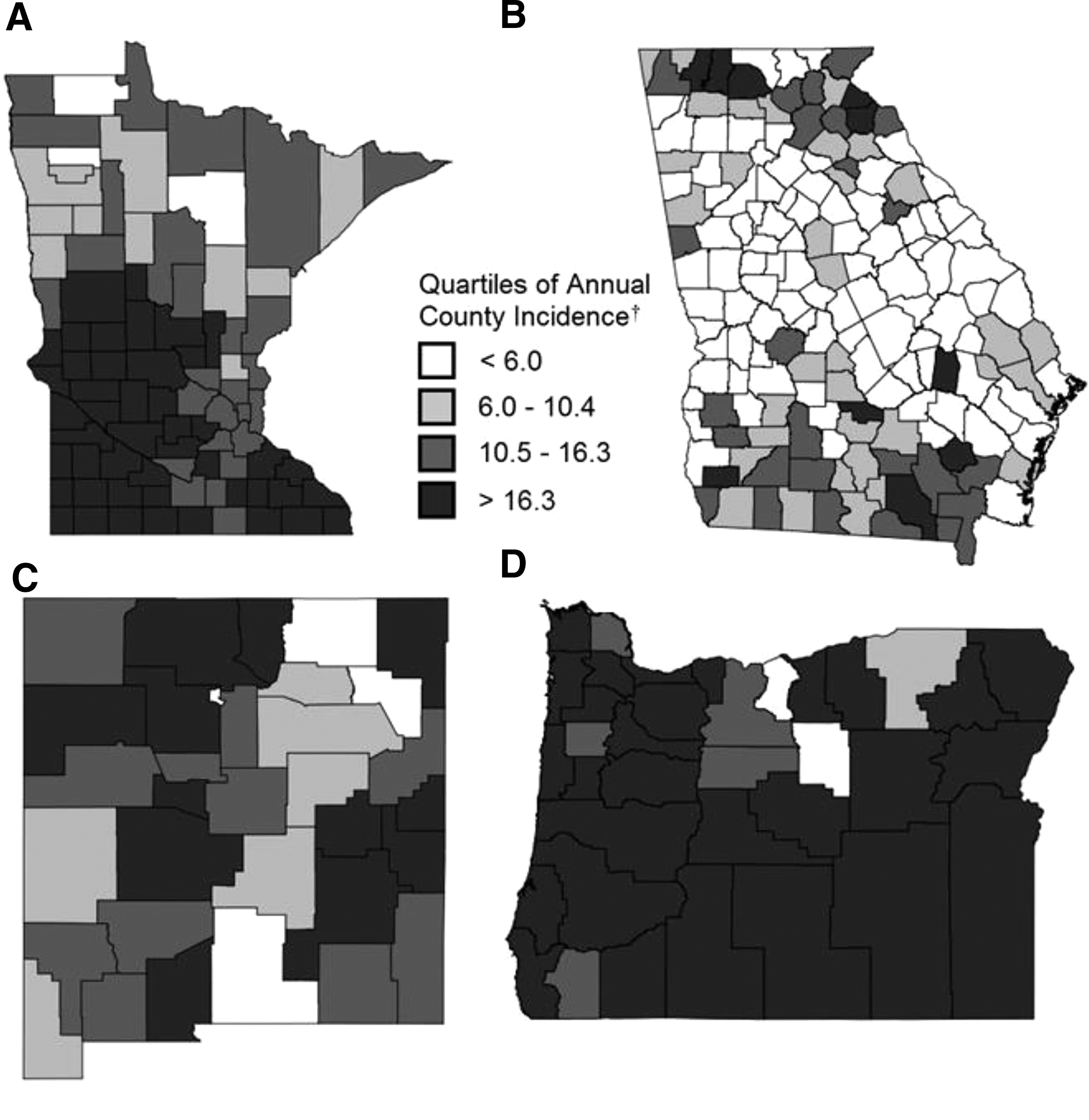
Observed county incidence per 100,000 in (A) Minnesota, (B) Georgia, (C) New Mexico, and (D) Oregon in 2011. Counties are shaded based on the quartiles of county annual incidence per 100,000.

Building models

Variance (1.71) and mean (0.43) of all the Campylobacter counts in the final dataset were calculated. The large variance relative to the mean suggested that the data were overdispersed (Rao and Sumathi, 2011). This was further supported by the NB's estimated overdispersion parameter [log(theta)], which was significantly different from zero with a p-value less than 0.001 (Cameron and Trivedi, 2013). The histogram in Figure 2 shows the case count frequency with a normal NB curve overlay (number of observations = 92,736, mean = 0.434, and theta = 0.213). Out of the 92,736 total subgroups, 78.6% had a zero case count. The curve mirrors the observed values closely and zero inflation is not apparent.

FIG. 2.

Count frequency of Campylobacter cases in FoodNet (bars) with normal negative binomial curve overlay (number of observations = 92,736, mean = 0.434, and theta = 0.213). Y axis is shown using a square-root scale.

Model results

All variables included in the nonzero-augmented models (NB and NB.Plus), both count and zero portions of the Hurdle models, and the count portion of the ZINB model were statistically significant predictors in the models. The ZINB Full was not included in the model comparison because none of the variables added by forward step selection was significant in the binary portion of the model. The individual model results are shown in Supplementary Appendix Table S1 (Supplementary Data are available online at www.liebertpub.com/fpd).

The count components of all models (NB, NB.Plus, Hurdle NB, Hurdle NB Full, and ZINB) had similar results in terms of coefficient direction, magnitude, and significance. However, Tennessee, year 2010, and age group 65+ were significant in the NB, NB.Plus, and the ZINB models, but not in the count components of the Hurdle NB and Hurdle NB Full models. The other difference was that the age group that includes 45–64 year olds was significant in the count component of the Hurdle NB and Hurdle NB Full models, but not in the count component of the ZINB model.

Model assessment and comparison

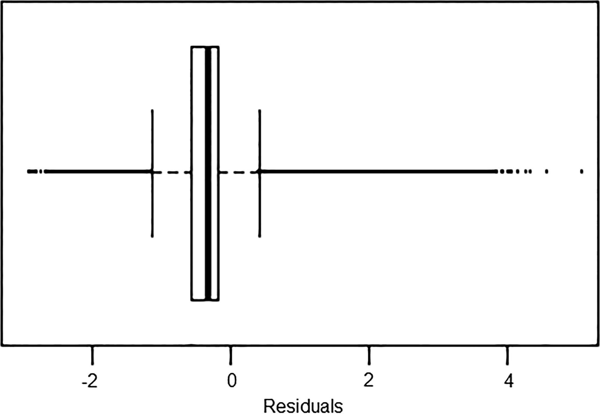
The zero component intercepts in the zero-augmented models had large negative coefficient values, which do not support the idea of zero inflation in the data. This is further supported by the goodness of fit evaluations summarized in Table 1. The likelihood ratio test led to the same results as the Vuong test when applied to nested models. Using the goodness of fit measures, the NB.Plus model had the best fit. The ZINB and NB.Plus had the same log likelihood, but different degrees of freedom. The Hurdle-NB model had the worst fit and the Hurdle NB Full had lower fit than both the ZINB and NB.Plus models. The residual histogram with a normal curve overlay is shown in Figure 3 for the NB.Plus model and displays deviation from homoscedasticity and normality.

FIG. 3.

Residual box plot of negative binomial model with demographic covariates (NB.Plus).

Table 1.

Goodness of Fit and Statistics Comparison by Model

Model 1^*
Model 2		Hurdle NB	NB	Hurdle NB full	ZINB	NB.Plus
M0†	LR		^***			^***
	V (BIC)	79.0^***	79.9^***	91.5^***	89.5^***	89.5^***
Hurdle NB	LR			^***
	V (BIC)		9.2^***	37.6^***	40.4^***	40.5^***
NB	LR					^***
	V (BIC)	−9.2^***		29.6^***	33.4^***	33.5^***
Hurdle NB full	LR	^***
	V (BIC)	−37.6^***	−29.6^***		3.7, 0.0001	3.9, 5.1e-5
ZINB	LR
	V (BIC)	−40.4^***	−33.4^***	(−3.7), 0.0001		174.2^***
NB.Plus	LR		^***
	V (BIC)	−40.5^***	−33.5^***	(−3.9), 5.1e-5	−174.2^***
−2 × log likelihood		−115,539	−114,403	−109,482	−109,525	−109,525
‡		25	17	47	25	24
AIC		115,589	114,437	109,576	109,575	109,573
BIC		115,825	114,597	110,019	109,811	109,799
MAE		0.3963	0.4046	0.3809	0.3798	0.3798
Predicted no. zeros		72,918	73,540	72,918	73,403	73,403

Models are listed from left to right and top to bottom as their fits improve; ^*Hurdle NB = Hurdle negative binomial with covariates in the count component only, NB = Negative binomial without demographic covariates, Hurdle NB Full = hurdle negative binomial with covariates in both zero and count components, ZINB = Zero-inflated negative binomial with covariates in the count component only, NB. Plus = Negative binomial with demographic covariates; †Null model; LR = Likelihood ratio test; V (BIC) = Vuong BIC corrected Non-Nested Hypothesis Test-Statistic; ^*** = p-value less than 2.2e-16 when testing model 1 versus model2 with alpha < 0.05; ‡Number of parameters estimated.

AIC, Akaike information criterion; BIC, Bayesian information criterion; MAE, Mean absolute error; NB, negative binomial.

Adding the demographic variables to the nonaugmented models decreased the mean absolute error by 0.0249 (decreased the error). For the zero-augmented NB.Plus model, the addition increased the mean absolute error by 2.726e-6 for the ZINB and by 0.0165 for the Hurdle NB model (increased the error). There were 72,918 zero case counts in the dataset, and the hurdle models predicted the exact number. When we rounded the predicted number of zeros to the nearest integer, both the ZINB and NB.Plus models predicted 73,403 zeros or 485 more than the observed number of zero counts. The hurdle models were superior at predicting zero counts because of their truncated structure.

Discussion

The aim of this analysis was to explore different methods to analyze campylobacteriosis case counts ascertained by FoodNet surveillance sites at a finer geographic level, evaluate the effect on incidence of covariates that may vary geographically, and examine the characteristics of zero counts in FoodNet Campylobacter data. The subgroups selected for analysis represented demographic and geographic variables known to influence incidence of Campylobacter infections (Ailes et al., 2008). Although a disproportionate number of observations were zero, zero inflation was not apparent, and the NB model with inclusion of demographic and seasonal variables significantly increased the fit of the model (see Table 1, NB.Plus) compared with the model with only year and state included (NB in Table 1). Our findings suggest that the incidence of Campylobacter infection varies substantially among the FoodNet counties, making it worthwhile to explore differences in surveillance populations, exposures, laboratory practices, or other factors that differ among sites.

Zero-augmented modifications (zero inflated and hurdle) of the regression models were used to examine a possible separation of observational and structural zeros. We anticipated that a significant proportion of zero case counts was observational; differences in county size and population demographics among the FoodNet surveillance sites result in very small subpopulation sizes among counties and a high probability that no cases will be observed among many counties. Our finding that the hurdle models did not fit the data well supports this assumption. Although we hypothesized that several surveillance and epidemiologic factors may contribute to structural zeros in the data, our analysis suggests that zero inflation is not apparent at the level of disaggregation of demographic covariates we studied; this finding is supported by the observation that inclusion of zero-augmentation mixing fractions did not improve the models' fit.

Although zero inflation was not present in the dataset, zero-augmented modeling techniques are likely to be important for future analyses, including modeling of other pathogens under FoodNet surveillance. Our models included only data ascertained by FoodNet active surveillance activities, and it is likely that inclusion of data from sites conducting passive surveillance, as well as data obtained from other sources, such as household income and access to healthcare, would contribute to the presence of structural zeros in the modeled data. The differences in data collection associated with different surveillance systems and data sources would likely result in excess zero case counts where at least a portion (structural zeros) arises from a process different from the positive counts. Although both hurdle and zero-inflated models may be used to model these types of data, it is likely best modeled by a zero-inflated model because the zeros are modeled as a mixture of both observational and structural zeros.

We removed the California observations because there were no zero case counts in any county subgroup, complicating our exploration of models for zero case counts. Removal of the California data eliminated convergence issues and allowed exploration of the effect of zero inflation. Removing the California data decreased the dataset's variance, but overdispersion was still prominent. An NB distribution helped in modeling the overdispersed data; however, there were still case counts that were outside the expected distribution. These case counts may be associated with undetected outbreaks (i.e., clusters of cases originating from a common exposure), which were not excluded from the analysis. Further exploration of these outliers, using compound distributions, would help better characterize them and might yield more information on risk factors of potential outbreaks (Hinde, 1982).

Conclusions

The addition of demographic and seasonal variables when modeling Campylobacter counts accounted for more variability and resulted in improved goodness of fit compared with models that only included a state factor. However, the complexity and variation in the epidemiology of Campylobacter were still not fully addressed, suggesting that differences in surveillance populations among the FoodNet sites or other epidemiological factors vary geographically. For example, the models did not fully account for the incidence variation among counties and states as illustrated in Figure 1. County-level variation associated with differences in county geographic size, population, and other unmeasured factors could result in additional sources of structural zeros in case counts. Although we investigated structural zeros at the state level, the possibility for structural zeros to vary by county was not examined. Potentially, the level of aggregation and count distribution could be adjusted per site to better fit the data and further explore structural zeros. Therefore, future steps should focus on individual sites.

Footnotes

Disclosure Statement

No competing financial interests exist.

References

Ailes

, Demma

, Hurd

, Hatch

, Jones

, Vugia

, Cronquist

, Tobin-D'Angelo

, Larson

, Laine

, Edge

. Continued decline in the incidence of Campylobacter infections, FoodNet 1996–2006. Foodborne Pathog Dis, 2008; 5:329–337.

Cameron

, Trivedi

. Regression Analysis of Count Data, 2nd edition. New York, NY: Cambridge University Press, 2013.

Desjardins

. Evaluating the performance of two competing models of school suspension under simulation-the zero-inflated negative binomial and the negative binomial hurdle. Dissertations University of Minnesota, 2013.

Erdman

, Jackson

, Sinko

. Zero-inflated poisson and zero-inflated negative binomial models using the COUNTREG procedure. In: Proceedings of the SAS Global Forum 2008 Conference, San Antonio, Texas. Cary, NC: SAS Institute Inc., 2008 pp.322–2008.

Gelman

, Hill

. Data Analysis Using Regression and Multilevel/Hierarchical Models. New York, NY: Cambridge University Press, 2006.

Henao

, Scallan

, Mahon

, Hoekstra

. Methods for monitoring trends in the incidence of foodborne diseases: Foodborne Diseases Active Surveillance Network 1996–2008. Foodborne Pathog Dis, 2010; 7:1421–1426.

Hinde

. Compound Poisson regression models. In Gilchrist

(ed.): GLIM 82: Proceedings of the International Conference on Generalised Linear Models. New York: Springer, 1982.

, Pavlicova

, Nunes

. Zero-inflated and hurdle models of count data with extra zeros: Examples from an HIV-risk reduction intervention trial. Am J Drug Alcohol Abuse, 2011; 37:367–375.

Kuhn

, Johnson

. Applied Predictive Modeling. New York: Springer, 2013.

10.

McCullagh

, Nelder

. Generalized Linear Models, 2nd edition. Boca Raton, FL: Chapman & Hall/CRC press, 1989.

11.

Mullahy

. Specification and testing of some modified count data models. J Econometrics, 1986; 33:341–365.

12.

QGIS Development Team. QGIS Geographic Information System. Open Source Geospatial Foundation Project;. 2013. Available at: http://qgis.osgeo.org Accessed August 12, 2015 .

13.

R Core Team. R: A Language and Environment for Statistical Computing. Vienna, Austria: R Foundation for Statistical Computing;. 2013. Available at: http://www.R-project.org Accessed June 14, 2105 .

14.

Rao

, Sumathi

. Selection of variables in regression models based on inflated distributions. Pakistan J Stat Oper Res, 2011; 7:381–390.

15.

Ridout

, Demétrio

CGB

, Hinde

. Models for count data with many zeros. In: Proceedings of the XIXth International Biometric Conference. Cape Town, South Africa: International Biometric Society, 1998, pp.179–192.

16.

Samuel

, Vugia

, Shallow

, Marcus

, Segler

, McGivern

, Kassenborg

, Reilly

, Kennedy

, Angulo

, Tauxe

. Epidemiology of sporadic Campylobacter infection in the United States and declining trend in incidence, FoodNet 1996–1999. Clin Infect Dis, 2004; 38(Supplement_3):S165–S174.

17.

Schwadel

, Falci

. Interactive effects of church attendance and religious tradition on depressive symptoms and positive affect. Soc Ment Health, 2012; 2:21–34.

18.

U.S. Census Bureau. Population Estimates. Intercensal and Postcensal Estimates by Year, State, County, Age, Sex, and Race, Prepared Under a Collaborative Arrangement with the US Census Bureau (2004–2011). Washington, DC: U.S. Census Bureau, 2011.

19.

Vuong

. Likelihood ratio tests for model selection and non-nested hypotheses. Econometrica, 1989; 57:307–333.

Supplementary Material

Please find the following supplemental material available below.

For Open Access articles published under a Creative Commons License, all supplemental material carries the same license as the article it is associated with.

For non-Open Access articles published, all supplemental material carries a non-exclusive license, and permission requests for re-use of supplemental material or any part of supplemental material shall be sent directly to the copyright owner as specified in the copyright notice associated with the article.

0.00 MB

0.11 MB