Evaluation of Grower-Friendly,Science-Based Sampling Approaches for the Detection of Salmonella in Ponds Used for Irrigation of Fresh Produce

Abstract

The recognition that irrigation water sources contribute to preharvest contamination of produce has led to new regulations on testing microbial water quality. To best identify contamination problems, growers who depend on irrigation ponds need guidance on how and where to collect water samples for testing. In this study, we evaluated several sampling strategies to identify Salmonella and Escherichia coli contamination in five ponds used for irrigation on produce farms in southern Georgia. Both Salmonella and E. coli were detected regularly in all the ponds over the 19-month study period, with overall prevalence and concentrations increasing in late summer and early fall. Of 507 water samples, 217 (42.8%) were positive for Salmonella, with a very low geometric mean (GM) concentration of 0.06 most probable number (MPN)/100 mL, and 442 (87.1%) tested positive for E. coli, with a GM of 6.40 MPN/100 mL. We found no significant differences in Salmonella or E. coli detection rates or concentrations between sampling at the bank closest to the pump intake versus sampling from the bank around the pond perimeter, when comparing with results from the pump intake, which we considered our gold standard. However, samples collected from the bank closest to the intake had a greater level of agreement with the intake (Cohen's kappa statistic = 0.53; p < 0.001) than the samples collected around the pond perimeter (kappa = 0.34; p = 0.009). E. coli concentrations were associated with increased odds of Salmonella detection (odds ratio = 1.31; 95% confidence interval = 1.10–1.56). All the ponds would have met the Produce Safety Rule standards for E. coli, although Salmonella was also detected. Results from this study provide important information to growers and regulators about pathogen detection in irrigation ponds and inform best practices for surface water sampling.

Introduction

In the United States, Salmonella causes ∼1 million cases of foodborne illness annually and the southeast consistently has high salmonellosis incidence rates (Scallan et al., 2011; CDC, 2014, 2016, 2017). Nationwide, nearly half salmonellosis cases can be attributed to produce (Painter et al., 2013). Crops can be contaminated throughout the farm-to-fork continuum, including the preharvest stages of production (Franz and van Bruggen, 2008; Tomás-Callejas et al., 2011; Park et al., 2012; Wadamori et al., 2017). Preharvest microbial contamination can occur through contact with pathogens in soil, animal feces, and irrigation water (Hanning et al., 2009; Gelting et al., 2011; Benjamin et al., 2013; Gelting and Baloch, 2013; Weller et al., 2015).

One common irrigation source is a farm pond, located adjacent to fields and replenished by streams, surface runoff, and groundwater from wells. Point and nonpoint sources of pond contamination can result in irrigation with contaminated water (Jokinen et al., 2010; Jacobsen and Bech, 2012; Gelting and Baloch, 2013; Gu et al., 2013; Weller et al., 2015; Antaki et al., 2016; Decol et al., 2017). Farm pond use may be especially concerning in regions where Salmonella spp. are regularly detected in surface waters, such as the southeast (Haley et al., 2009; Rajabi et al., 2011; Li et al., 2014; Strawn et al., 2014; Luo et al., 2015; Maurer et al., 2015).

In 2015, the Produce Safety Rule (PSR) of the Food Safety Modernization Act (FDA, 2015) provided growers with numerical water quality criteria for untreated agricultural water. However, it did not provide directions for how and where to obtain pond water samples that would best represent irrigation water quality. Pond water is withdrawn through intake pipes using pumps usually located on pond banks. Water near the intake likely best represents irrigation water quality but the intake is often difficult to access from the bank. Thus, growers must make critical decisions regarding water sampling to accurately assess agricultural water quality.

To provide guidance on sampling for PSR compliance, we compared strategies for sampling irrigation ponds in southern Georgia. PSR criteria are for generic Escherichia coli but we extended our analysis to Salmonella spp. because earlier studies by our team found Salmonella in these ponds (Li et al., 2014; Luo et al., 2014, 2015; Harris et al., 2018). We assessed water quality at five ponds analyzed by Li et al. (2014) and two ponds analyzed by Harris et al. (2018), adding new water quality data not previously reported in those studies.

Materials and Methods

Sample collection

We sampled five irrigation ponds on commercial produce farms in southern Georgia monthly from March 2012 to September 2013 (Fig. 1 and Table 1). Because of the large distances between farms, ponds were visited on a rotational basis, with two ponds (CC2 and MD1) sampled during the first week of the month, and three ponds (NP, LV, and SC1) sampled during the third week. At each visit, we sampled the water surface directly above the pump intake, which we considered the “gold standard” for irrigation water quality because it was where water entered the irrigation distribution system (Fig. 2). Because of sampling feasibility, sampling strategies were alternated between months. For strategy 1, three 4.5-L grab samples, ∼3 m apart, were collected at the edge of the pond near the intake. For strategy 2, 4.5-L grab samples were collected at three fixed, accessible locations along the pond's perimeter: near the intake, on the pond dam, and a third point equidistant to the other two locations. These sampling points were selected to represent the landscape surrounding the pond. For both strategies, 1.5-L aliquots from grab samples were combined to create a composite sample. From March to September 2013, in addition to sampling the intake at the water surface, a sample was collected closer to the intake, 0.5 m below the surface. Sampling strategies are given in Figure 3. A total of 507 samples were collected. On three occasions, water levels at CC2 were too low to collect the full set of samples.

FIG. 1.

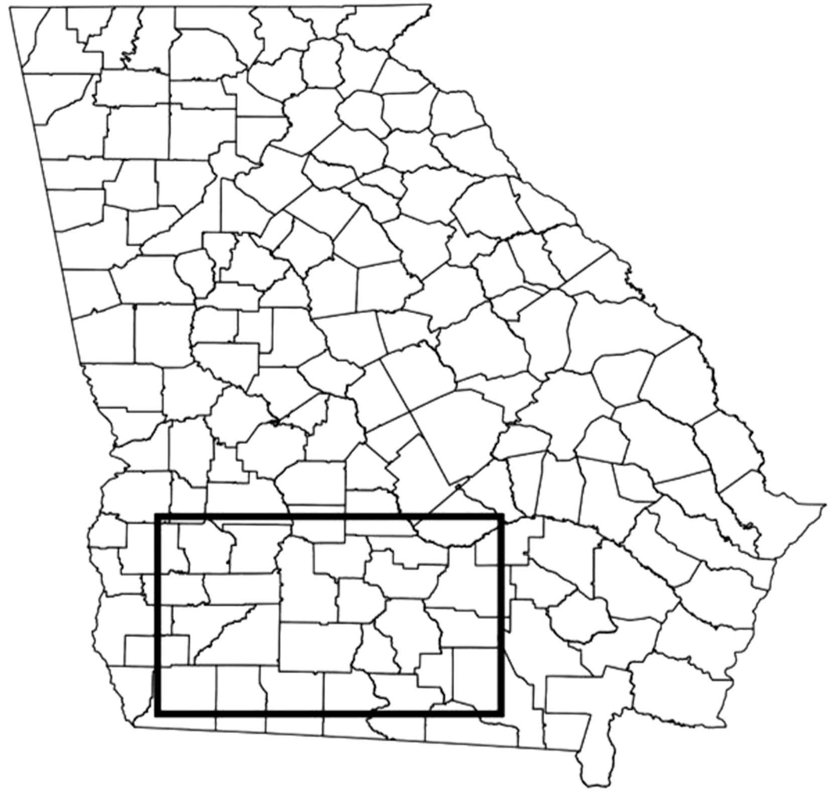
Map of Georgia with the rectangle indicating the geographic region within which the five ponds were located.

FIG. 2.

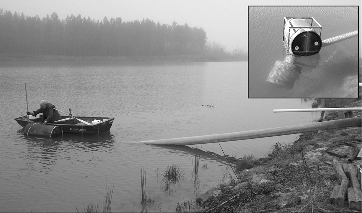
Collecting samples at the pump intake of pond NP. The screened intake at the end of the intake pipe is suspended between 1 and 2 m below the surface with the support of a plastic drum. The inset shows the intake.

FIG. 3.

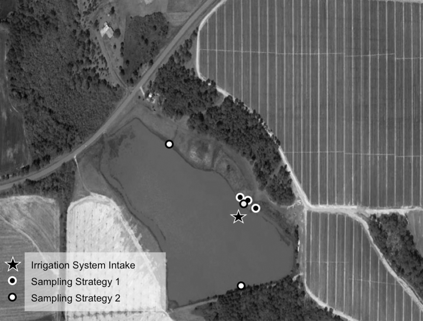
Example of sampling strategies at one pond. All sampling events included a sample near the intake of the pump (star) that served as the gold standard for comparison. For sampling strategy 1, three grab samples were collected from the edge of the pond, near the intake of the pump. For sampling strategy 2, three grab samples were collected from the edge of the pond, around the pond's perimeter.

Table 1.

Summary of the Five Irrigation Ponds Surveyed

Pond	N	Salmonella GM concentrations (% positive)	Escherichia coli GM concentrations (% positive)	Pond area (m²)	Watershed area (m²)	Land use–cropland (%)	Land use–forest/wetland (%)
CC2	99	0.08 (53)	14.91 (96)	21,637	877,759	57.3	33.7
LV	102	0.05 (39)	5.02 (83)	5799	6822	81.0	15.2
MD1	102	0.07 (49)	3.78 (71)	10,955	204,309	28.8	31.3
NP	102	0.04 (28)	6.15 (91)	46,722	658,244	36.8	53.8
SC	102	0.06 (45)	6.31 (95)	79,935	2,745,691	42.9	40.4
Total	507	0.06 (43)	6.40 (87)

For each irrigation pond, the size of the pond and watershed, the predominant composition of the area within a 250 m radius of each pond edge in terms of land use type (% coverage), and summary of the prevalence and geometric mean (GM) concentrations of Salmonella spp. and Escherichia coli are provided.

GM, geometric mean.

Samples were placed on ice and analyzed in the laboratory within 24 h. In situ measurements of pH, temperature, dissolved oxygen, turbidity, and specific conductivity were taken using a YSI model 6920 multiprobe data sonde (YSI Incorporated, Yellow Springs, OH).

Sample analysis

Salmonella concentrations were enumerated with a culture-based most probable number (MPN) method using three dilution volumes (Luo et al., 2014). In triplicate, water samples (500, 100, and 10 mL) were enriched with equal volumes of 2 × lactose broth (Becton, Dickinson and Company [BD] Difco™, Franklin Lakes, NJ) and incubated at 37°C for 24 h. Then, 1 mL of each culture (nine total for each sample) was added to 9 mL of Salmonella-selective tetrathionate broth with iodine (Thermo Scientific™; Remel™, Lenexa, KS) and incubated at 37°C for 24 h. Cultures were streaked onto xylose-lysine-Tergitol-4 (BD) agar and CHROMagar™ Salmonella Plus (CHROMagar Microbiology, Paris, France). Presumptive positive samples were inoculated into Luria–Bertani broth (BD) and incubated at 37°C for 24 h. One-milliliter cultures were boiled at 100°C for 10 min and then centrifuged at 14,000 g for 5 min. Supernatants were analyzed with PCR targeting the invA gene (Chiu and Ou, 1996). The lower limit of detection (LOD) was 0.0548 MPN/100 mL and the upper LOD was 11 MPN/100 mL. Total coliforms and E. coli were enumerated using the Quanti-Tray/2000 System with Colilert Reagent (IDEXX Laboratories, Westbrook, ME). The lower and upper LOD were 1 MPN/100 mL and 2419.6 MPN/100 mL, respectively. Total suspended solids were analyzed with a colorimetric autoanalyzer.

Statistical analysis

Concentrations below the LOD were assigned a value of half the LOD. Concentrations above the upper LOD were set to the LOD. To address skewness, we log₁₀-transformed Salmonella and E. coli concentrations. For presence/absence analysis, concentrations below the LOD were considered to have an absence of Salmonella or E. coli.

Spatiotemporal differences in concentrations and prevalence for Salmonella and E. coli were assessed. Pearson's chi-square tests were used to compare microbial prevalence in each strategy, irrigation pond, and month. Tukey's honest significant difference tests were used to compare concentrations at the 95% familywise confidence level between strategies, ponds, and months.

The strategies (shoreline sampling near the intake vs. around the perimeter) were evaluated by comparing the presence of Salmonella and E. coli in edge samples with the intake (“gold standard”). Composite and edge sample agreements with the intake were compared to determine whether a composite sample was comparable with three discrete samples. One method for comparing strategies was to estimate agreement between edge/composite and intake samples by calculating the percentage of edge/composite samples that matched the intake. Another method was to calculate Cohen's kappa coefficient (Cohen, 1960) for agreement between edge/composite samples with the intake. Instead of comparing individual edge samples to the intake, edge sample data were aggregated for each strategy so that Salmonella or E. coli detection in any edge sample rendered the aggregated edge sample positive for Salmonella or E. coli. The third method was to estimate pond misclassification using shoreline samples, assuming the intake accurately reflected irrigation water quality. Samples matching the intake for Salmonella or E. coli presence were considered “true positives” (TP) or “true negatives” (TN), whereas samples not matching the intake were considered “false negatives” (FN) or “false positives” (FP). The FP rate was calculated using: FP/(FP + TN). The FN rate was calculated using FN/(FN + TP).

Associations between potential predictors of water quality and Salmonella presence were modeled with a logistic regression with random effects for pond. E. coli concentrations and presence were considered predictors because of their inclusion in previous studies (McEgan et al., 2013; Partyka et al., 2018). The following physicochemical parameters were considered: turbidity, suspended solids, specific conductivity, oxidation–reduction potential, pH, and temperature. Temporal effects were controlled with a variable for month. Statistical analyses were performed in R 3.1.3 (R Core Team, 2015).

Scenario testing for study ponds

Although this study was conducted before the PSR went into effect, we examined the hypothetical scenario of testing ponds for PSR compliance. The PSR requires an initial survey of E. coli, in which the geometric mean (GM) of at least 20 samples must not exceed 126 colony-forming units (CFU)/100 mL and the statistical threshold value (STV), approximating the 90th percentile of a normal distribution (z-score = 1.28), must not exceed 410 CFU/100 mL. This study utilized MPN methods for enumeration and was thereby unable to quantify E. coli in terms of CFU. Because of evidence that MPN and CFU values in paired samples were not significantly different, our MPN values were compared with CFU criteria (IDS Decision Sciences, 2017).

For each pond, we calculated the E. coli GMs and STVs in two ways: (1) using all values from the study period and (2) selecting 20 of the highest values to simulate a worst-case scenario. In addition to comparing the GM/STV with PSR criteria, we determined the number of samples whose indicator results disagreed with the pathogen results. We refer to samples that were Salmonella-positive although E. coli levels were below the standard as FN and samples that were Salmonella-negative when E. coli levels exceeded the standard as FP. For PSR-compliant ponds, we calculated the FN rate as (no. of Salmonella-positive samples)/(no. of samples). For PSR-noncompliant ponds, we calculated the FP rate as (no. of Salmonella-negative samples)/(no. of samples).

Results

A total of 217 (42.8%) samples were Salmonella positive, with a GM of 0.06 MPN/100 mL (STV: 0.25 MPN/100 mL) and 442 (87.1%) were E. coli positive, with a GM of 6.40 MPN/100 mL (STV: 61.4 MPN/100 mL). Microbiological water quality results are given in Table 1.

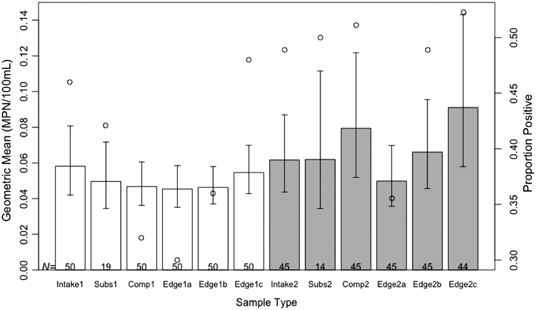
There were no significant differences in Salmonella prevalence or concentrations between the intake, edge, and composite samples (Fig. 4). This was also true for E. coli (Supplementary Fig. S1; Supplementary Data are available online at www.liebertpub.com/fpd). Agreement levels between edge, composite, and intake samples were similar for both strategies (Table 2). For Salmonella, agreement levels were highest between strategy 1's edge and intake samples, whereas for E. coli, agreement levels were highest between strategy 2's edge and intake samples.

FIG. 4.

Comparison of Salmonella spp. concentrations by sampling strategy, stratified by the different sample types within each strategy. The bar plot compares the GM of Salmonella concentrations (left y-axis) for each sample type. “Comp” corresponds to the composite sample, created by combining aliquots of the three edge samples. “Intake” refers to the sample collected at the surface of the pond directly above the intake pump (considered the gold standard), whereas “subs” samples were collected below the surface of the pond but above the intake pump. For each strategy (differentiated by color: white for strategy 1 [bank sampling closest to the intake], gray for strategy 2 [bank sampling at three locations around the perimeter of the pond]), three edge samples (a–c) were collected. Composite, edge, intake, and subsurface samples are numbered according to their associated strategy (1 or 2). Error bars represent the standard error around the GM. The scatter plot of open circles compares the proportion of positive samples (right y-axis) for each sample type. Sample sizes are indicated at the bottom of each bar. GM, geometric mean.

Table 2.

Presence/Absence Agreement for (a) Salmonella spp. and (b) Escherichia coli.

	Composite, %	Intake, %
(a) Salmonella
Intake 1	70.0	—
Intake 2	71.1	—
Edge 1 (grouped)	70.0	76.0
Edge 2 (grouped)	64.4	66.7
(b) Escherichia coli
Intake 1	84.0	—
Intake 2	88.9	—
Edge 1 (grouped)	88.0	80.0
Edge 2 (grouped)	93.3	91.1

Samples were compared to others within the same strategy, e.g., Intake 1 was compared to Composite 1 and Edge 1 while Intake 2 was compared to Composite 2 and Edge 2. Sampling strategies are described in the text.

When comparing Salmonella presence in edge/composite samples with intake samples using Cohen's kappa, strategy 1 edge samples had the highest coefficient of 0.53 (p < 0.001). For E. coli, compared with strategy 1, strategy 2 edge samples were more consistent with the intake—edge and composite samples had coefficients of 0.56 (p < 0.001) and 0.49 (p < 0.001), respectively. Kappa coefficients for edge/composite agreement with the intake are given in Table 3.

Table 3.

Cohen's Kappa Coefficients for the Agreement of Results Between Edge/Composite and Intake Samples for Strategy 1 and Strategy 2

	Intake
(a) Salmonella
Strategy 1
Edge	0.53 (p < 0.001)
Composite	0.38 (p = 0.005)
Strategy 2
Edge	0.34 (p = 0.009)
Composite	0.42 (p = 0.005)
(b) Escherichia coli
Strategy 1
Edge	−0.04 (p = 0.636)
Composite	0.41 (p = 0.004)
Strategy 2
Edge	0.56 (p < 0.001)
Composite	0.49 (p < 0.001)

Kappa coefficient	Agreement level
<0.00	Poor
0.00–0.20	Slight
0.21–0.40	Fair
0.41–0.60	Moderate
0.61–0.80	Substantial
0.81–1.00	Almost perfect

Coefficients for a) Salmonella spp. presence and b) Escherichia coli presence are shown. The legend below the graph provides guidelines for the interpretation of kappa coefficient magnitude (Landis and Koch 1977).

For both strategies, individual edge and composited samples had high rates (27.3–56.5%) of FN misclassifications of the intake (Table 4). For E. coli, the edge/composite samples of both sampling strategies had lower FN rates of 2.4–7.3%. Aggregating the results of multiple edge samples reduced the FN rates for Salmonella (8.7–9.1%) and E. coli (0–2.4%). Strategy 1 performed marginally better than strategy 2 in lowering Salmonella FN rates (8.7% vs. 9.1%) but for E. coli, the opposite was true (0% vs. 2.4%).

Table 4.

Performance of Sampling Strategies Compared to the Intake (Gold Standard) in Detecting Salmonella spp. and Escherichia coli

	Salmonella		Escherichia coli
	False negatives, %	False positives, %	False negatives, %	False positives, %
Composite 1	47.8	14.8	7.3	55.6
Edge 1 (grouped)	8.7	37.0	2.4	100.0
Edge 1a	47.8	11.1	2.4	44.4
Edge 1b	56.5	18.5	2.4	55.6
Edge 1c	34.8	33.3	7.3	77.8
Composite 2	27.3	30.4	2.6	57.1
Edge 2 (grouped)	9.1	56.5	0	57.1
Edge 2a	45.4	17.4	2.6	42.9
Edge 2b	31.8	30.4	5.3	42.9
Edge 2c	45.5	50.0	5.4	42.9

Sampling strategies are described in the text. Edge 1 (grouped) and Edge 2 (grouped) represent whether any of the three edge (a, b, c) samples were positive for Salmonella/E. coli.

There were significant differences in Salmonella concentrations between ponds (Fig. 5; Supplementary Table S1). CC2 had the highest mean concentration, significantly higher than two ponds (NP: difference = 0.74 log MPN/100 mL, p adj <0.001; LV: difference = 0.49 log MPN/100 mL, p adj = 0.015). NP had the lowest concentration, significantly lower than three ponds (CC2: see above; MD1: difference = 0.64 log MPN/100 mL, p adj <0.001; SC: difference = 0.48 log MPN/100 mL, p adj = 0.018). There were also significant differences in Salmonella prevalence (χ² = 14.7935, df = 4, p = 0.005). E. coli levels were significantly greater at CC2 than at other ponds (maximum difference between MD1 and CC2: 1.37, p adj <0.001).

FIG. 5.

Comparison of Salmonella spp. concentrations (bar plot; left y-axis) and proportion of samples positive for Salmonella (open circles; right y-axis) among the five ponds in this study (CC2, LV, MD1, NP, and SC). Significant differences between geometric means of individual ponds are indicated below the plot.

Salmonella concentrations peaked in October and prevalence peaked in September (Fig. 6). E. coli seasonality differed slightly from that of Salmonella; the peak of concentrations occurred in July and E. coli was regularly detected in more than half the samples (Supplementary Fig. S2).

FIG. 6.

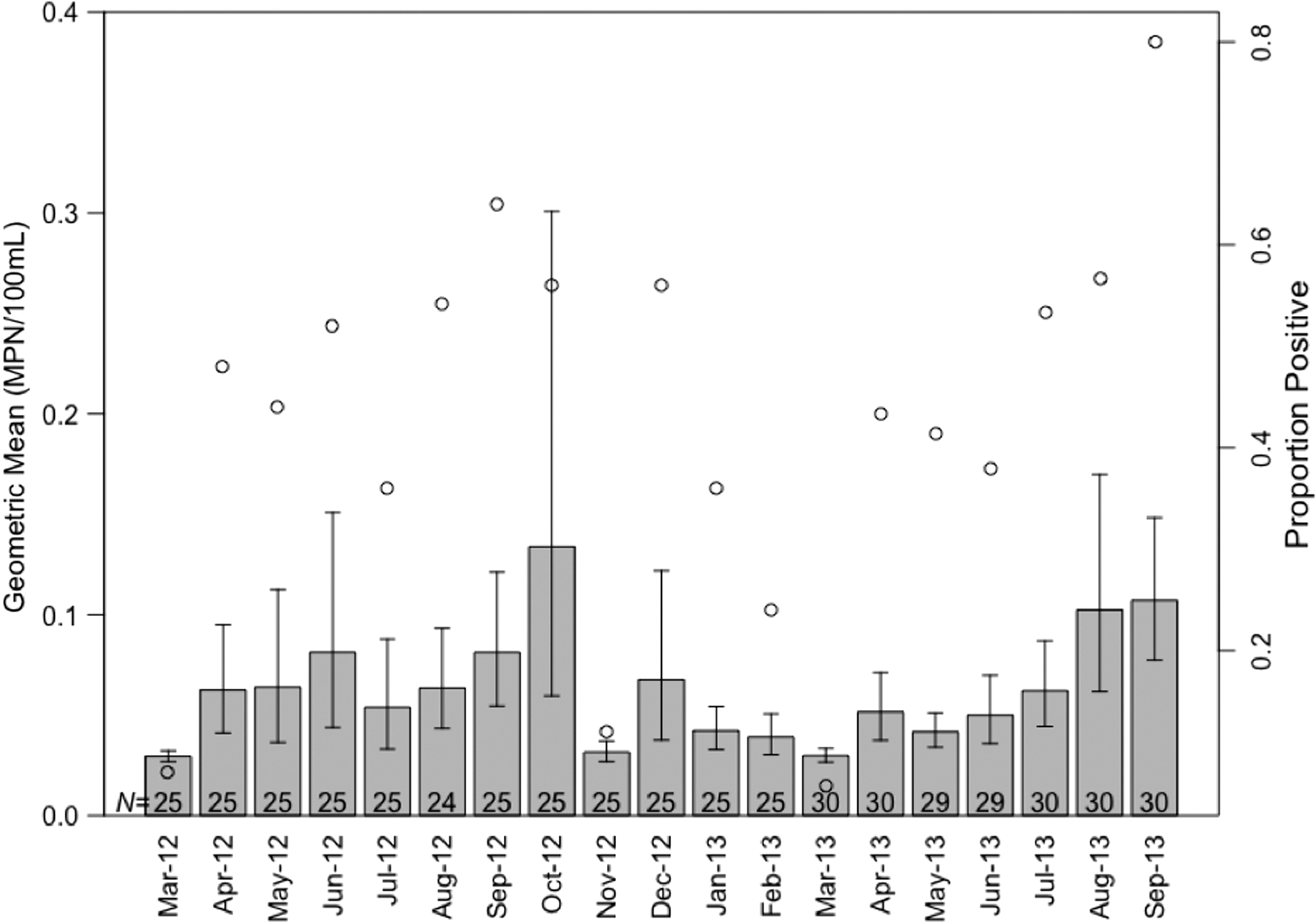
Seasonal trend of Salmonella spp. concentrations (bar plot; left y-axis) and proportion of samples positive for Salmonella (open circles; right y-axis) during the 19-month study period (March 2012–September 2013). Sample sizes are given at the base of the bars.

E. coli concentrations were associated with increased odds of Salmonella detection. A 1-log increase in E. coli concentration was associated with a 31% increase in the odds of Salmonella presence (odds ratio = 1.31; 95% confidence interval [CI] = 1.10–1.56). E. coli presence was not associated with increased odds (odds ratio = 0.94; 95% CI = 0.37–2.39). Physicochemical parameters were not associated with Salmonella presence. Odds ratios for predictors are given in Supplementary Table S2.

At all ponds, E. coli GMs (highest GM: 14.91 MPN/100 mL at CC2) and STVs (highest STV: 67.5 MPN/100 mL at LV) met PSR standards. In the worst-case scenario, two ponds (CC2 and LV) exceeded standards (LV: GM = 145.4 MPN/100 mL, STV = 693.8 MPN/100 mL; CC2: GM = 150.9 MPN/100 mL, STV = 747.1 MPN/100 mL). In this worst-case scenario, three ponds (MD1, NP, and SC) would have been PSR compliant, yet we detected Salmonella in all ponds. Deeming ponds Salmonella negative would have yielded FN results in 80% of MD1, 100% of NP, and 60% of SC samples.

Discussion

Every month, Salmonella was detected—at low concentrations—in at least one pond. Nearly 90% of pond samples had detectable E. coli, and increases in E. coli concentrations were associated with increased odds of detecting Salmonella. All ponds would have been considered safe for agricultural use per PSR's E. coli-based standards; however, Salmonella was detected at all ponds.

When comparing two shoreline-sampling strategies for Salmonella, we found no statistical difference between sampling near the intake versus around the perimeter. Even so, the agreement in Salmonella presence between strategy 1 samples suggests that it may be marginally better than strategy 2 at approximating intake water quality. This was likely the result of the proximity of this sampling location to the intake. Salmonella and E. coli have different microhabitat and physicochemical preferences in surface water (Mugnai et al., 2015; Partyka et al., 2018) and thus, water from the same pond area (e.g., near the intake) may share factors promoting microbial survival. The edge samples collected near the intake were similar in Salmonella and E. coli concentrations.

However, the edge samples around the perimeter varied in Salmonella and E. coli concentrations, suggesting spatial heterogeneity of microbes in our ponds. Furthermore, neither shoreline-sampling strategy had high agreement levels with the intake. Compared with shoreline samples, the intake (located at the pond's interior) generally had lower concentrations of E. coli, similar to a recent finding in California (Pachepsky et al., 2018). Shoreline Salmonella concentrations, on the contrary, did not trend higher or lower than the concentrations at the intake, suggesting that Salmonella and E. coli may have different drivers of lateral distribution in ponds. Again, the location and physicochemical parameter preferences of Salmonella and E. coli may have driven within-pond variations in concentrations (Mugnai et al., 2015; Partyka et al., 2018).

One study limitation was our consideration of water above the intake as the “gold standard” for irrigation water quality. Previous studies of surface water have also focused on intake sampling (Gu et al., 2013; Li et al., 2014; Luo et al., 2015; Antaki et al., 2016), but the intake may not reflect the quality of water applied to crops or even the overall quality of the pond—only water quality near the intake in one instance. Intake water quality may reflect water quality at the beginning of irrigation events but eventually, water from other regions of the pond will be pumped out for irrigation. We were unable to control the timing of irrigation events but were able to sample during pump operation on six occasions. Another limitation was the location of intake sampling. Because of sampling feasibility, we did not sample water within the intake pipe; we sampled at the water surface and for the last 7 months of the study, 0.5 m below the surface, closer to the intake. It may be more informative for growers to analyze water within the irrigation distribution system. This may also be preferable because biofilm formation within the intake pipe (Pachepsky et al., 2012; Blaustein et al., 2015) could result in the use of contaminated water even when ponds are deemed suitable for irrigation.

We found that E. coli concentrations were associated with increased odds of detecting Salmonella. Studies of indicator–pathogen relationships have conflicting findings; some studies have found that generic E. coli is a poor indicator (Haley et al., 2009; Wilkes et al., 2009; Ahmed et al., 2010; Jenkins et al., 2012; Cerna-Cortes et al., 2013), whereas others have found that, similar to this study, E. coli concentrations are associated with Salmonella presence (McEgan et al., 2013; Partyka et al., 2018).

Although there is evidence of a relationship between Salmonella and E. coli, Salmonella is often detected in surface water that meets E. coli-based standards. This was observed not only in areas in this study but also in California (Benjamin et al., 2013; Partyka et al., 2018) and Florida (McEgan et al., 2013; Topalcengiz et al., 2017). One explanation for this weak correlation might be that the factors mediating the survival and transport of Salmonella and E. coli differ. Our results show that E. coli levels peak in early- to mid-summer, concurrent with peak temperatures, whereas Salmonella concentrations peaked in late summer/early fall. This seasonal Salmonella peak was also observed in other surface water surveys in this region (Haley et al., 2009; Luo et al., 2015; Antaki et al., 2016), indicating that Salmonella concentrations might be driven by factors other than temperature. In the fall in Georgia, there may be increased activity of animal reservoirs of Salmonella (Srikantiah et al., 2004; Jokinen et al., 2010, 2011; Maurer et al., 2015) or the transport of Salmonella introduced into the environment through septic leakage in the summer, when salmonellosis incidence increases (Sowah et al., 2014; Verhougstraete et al., 2015; CDC, 2017).

Limitations of this study include the low number and limited geographic range of ponds sampled. However, the general principles related to optimizing pond sampling strategies are relevant to any farm relying on surface water irrigation sources, especially farms in regions where Salmonella spp. are regularly detected. In California, Salmonella is detected in surface water at low prevalence rates (Gorski et al., 2011; Benjamin et al., 2013). In the southeast, prevalence varies but has been detected in up to 79% of samples in Georgia (Haley et al., 2009) and up to 100% in Florida (McEgan et al., 2013). In our study, Salmonella was detected in 43% of samples, similar to the prevalence rates (33–37%) detected by Luo et al. (2015) and Harris et al. (2018) who used the same methodology in a similar geographic area. In contrast, the 12% prevalence detected by Antaki et al. (2016) in this region was similar to prevalence rates detected in California. The lower prevalence rates detected in these studies may have resulted from the use of different Salmonella detection methods.

Despite the differences in prevalence, studies of surface water in agricultural regions of California (Gorski et al., 2011; Benjamin et al., 2013; Walters et al., 2013), Florida (Rajabi et al., 2011; McEgan et al., 2013; Strawn et al., 2014), Georgia (Li et al., 2014; Maurer et al., 2015; Antaki et al., 2016), and New York (Strawn et al., 2014) indicate the widespread presence of Salmonella in surface water and the concomitant risks of irrigating with surface water. Growers in California rely on groundwater for irrigation because of the greater availability and microbiological quality of groundwater but sometimes store groundwater in open reservoirs that can become contaminated (Benjamin et al., 2013) and thus, issues related to surface water quality are highly relevant to these growers as well. This study's detection of spatial heterogeneity of pond microbes and the limitations of E. coli as an indicator organism warrant further research to improve irrigation water quality standards.

Conclusions

Our findings suggest that growers should ideally sample at the pump intake but shoreline sampling near the intake may be an adequate alternative. Aggregating data from multiple samples (compared with a composite) would increase Salmonella detection agreement levels between the shore and the intake. We detected Salmonella in ponds used for produce irrigation but the health risk to consumers is unclear given the low concentrations detected. Although the PSR may be appropriate in regions where Salmonella is not prevalent in the environment, future studies focusing on the southeast—where Salmonella and salmonellosis prevalence are high—will be crucial in providing science-based improvements to the PSR and promoting produce safety nationwide.

Footnotes

Acknowledgments

The authors thank the growers involved in this study for allowing us to access these ponds. The authors also thank Debbie Coker, Herman Henry, Charles Gruver, Catherine (Katy) Summers, and T.J. Hines for their technical assistance in the laboratory and field.

Funding

This study was supported through a grant from the Center for Produce Safety (Award no.: 2012-186; http://bit.ly/2DklsJg). K.L. is supported by the National Institute for Allergy and Infectious Diseases, NIH (grant no. 1K01AI103544). The content is solely the responsibility of the authors and does not necessarily represent the official views of the funders.

Disclosure Statement

No competing financial interests exist.

References

Ahmed

, Goonetilleke

, Gardner

. Implications of faecal indicator bacteria for the microbiological assessment of roof-harvested rainwater quality in southeast Queensland, Australia. Can J Microbiol, 2010; 56:471.

Antaki

, Vellidis

, Harris

, Aminabadi

, Levy

, Jay-Russell

. Low concentration of Salmonella enterica and generic Escherichia coli in farm ponds and irrigation distribution systems used for mixed produce production in Southern Georgia. Foodborne Pathog Dis, 2016; 13:551–558.

Benjamin

, Atwill

, Jay-Russell

, Cooley

, Carychao

, Gorski

, Mandrell

. Occurrence of generic Escherichia coli, E. coli O157 and Salmonella spp. in water and sediment from leafy green produce farms and streams on the Central California coast. Int J Food Microbiol, 2013; 165:65–76.

Blaustein

, Shelton

, Van Kessel

JAS

, Karns

, Stocker

, Pachepsky

. Irrigation waters and pipe-based biofilms as sources for antibiotic-resistant bacteria. Environ Monit Assess, 2015; 188:56.

[CDC] The Centers for Disease Control and Prevention. National Salmonella Surveillance Annual Report, 2012. Atlanta, GA: U.S. Department of Health and Human Services, CDC, 2014.

CDC. National Salmonella Surveillance Annual Report, 2013. Atlanta, GA: U.S. Department of Health and Human Services, CDC, 2016.

CDC. Foodborne Diseases Active Surveillance Network (FoodNet): FoodNet 2015 Surveillance Report (Final Data). Atlanta, GA: U.S. Department of Health and Human Services, CDC, 2017.

Cerna-Cortes

, Gómez-Aldapa

, Rangel-Vargas

, Ramírez-Cruz

, Castro-Rosas

. Presence of indicator bacteria, Salmonella and diarrheagenic Escherichia coli pathotypes on mung bean sprouts from public markets in Pachuca, Mexico. Food Control, 2013; 31:280–283.

Chiu

, Ou

. Rapid identification of Salmonella serovars in feces by specific detection of virulence genes, invA and spvC, by an enrichment broth culture-multiplex PCR combination assay. J Clin Microbiol, 1996; 34:2619–2622.

10.

Cohen

. A coefficient of agreement for nominal scales. Educational Psychol Meas, 1960; 20:37–46.

11.

Decol

, Casarin

, Hessel

, Batista

ACF

, Allende

, Tondo

. Microbial quality of irrigation water used in leafy green production in Southern Brazil and its relationship with produce safety. Food Microbiol, 2017; 65:105–113.

12.

[FDA] U.S. Food and Drug Administration. Final Rule on Produce Safety. Washington, DC: U.S. Food and Drug Administration, 2015.

13.

Franz

, van Bruggen

AHC

. Ecology of E. coli O157:H7 and Salmonella enterica in the primary vegetable production chain. Crit Rev Microbiol, 2008; 34:143–161.

14.

Gelting

, Baloch

. A systems analysis of irrigation water quality in environmental assessments related to foodborne outbreaks. Aquat Procedia, 2013; 1:130–137.

15.

Gelting

, Baloch

, Zarate-Bermudez

, Selman

. Irrigation water issues potentially related to the 2006 multistate E. coli O157:H7 outbreak associated with spinach. Agric Water Manage, 2011; 98:1395–1402.

16.

Gorski

, Parker

, Liang

, Cooley

, Jay-Russell

, Gordus

, Atwill

, Mandrell

. Prevalence, distribution, and diversity of Salmonella enterica in a major produce region of California. Appl Environ Microbiol, 2011; 77:2734–2748.

17.

, Luo

, Cevallos-Cevallos

, Adams

, Vellidis

, Wright

, van Bruggen

AHC

. Factors affecting the occurrence of Escherichia coli O157 contamination in irrigation ponds on produce farms in the Suwannee River Watershed. Can J Microbiol, 2013; 59:175–182.

18.

Haley

, Cole

, Lipp

. Distribution, diversity, and seasonality of waterborne Salmonellae in a rural watershed. Appl Environ Microbiol, 2009; 75:1248–1255.

19.

Hanning

, Nutt

, Ricke

. Salmonellosis outbreaks in the United States due to fresh produce: Sources and potential intervention measures. Foodborne Pathog Dis, 2009; 6:635–648.

20.

Harris

, Tertuliano

, Rajeev

, Vellidis

, Levy

. Impact of storm runoff on Salmonella and Escherichia coli prevalence in irrigation ponds of fresh produce farms in southern Georgia. J Appl Microbiol, 2018; 124:910–921.

21.

IDS Decision Sciences. Report on Agricultural Water Testing Methods Colloquium. Irvine, CA: Center for Produce Safety, 2017.

22.

Jacobsen

, Bech

. Soil survival of Salmonella and transfer to freshwater and fresh produce. Food Res Int, 2012; 45:557–566.

23.

Jenkins

, Endale

, Fisher

, Paige Adams

, Lowrance

, Larry Newton

, Vellidis

. Survival dynamics of fecal bacteria in ponds in agricultural watersheds of the Piedmont and Coastal Plain of Georgia. Water Res, 2012; 46:176–186.

24.

Jokinen

, Edge

, Ho

, Koning

, Laing

, Mauro

, Medeiros

, Miller

, Robertson

, Taboada

, Thomas

, Topp

, Ziebell

, Gannon

VPJ

. Molecular subtypes of Campylobacter spp., Salmonella enterica, and Escherichia coli O157: H7 isolated from faecal and surface water samples in the Oldman River watershed, Alberta, Canada. Water Res, 2011; 45:1247–1257.

25.

Jokinen

, Schreier

, Mauro

, Taboada

, Isaac-Renton

, Topp

, Edge

, Thomas

, Gannon

VPJ

. The occurrence and sources of Campylobacter spp., Salmonella enterica and Escherichia coli O157: H7 in the Salmon River, British Columbia, Canada. J Water Health, 2010; 8:374–386.

26.

Landis

, Koch

. The measurement of observer agreement for categorical data. Biometrics, 1977; 33:159–174.

27.

, Vellidis

, Liu

, Jay-Russell

, Zhao

, Hu

, Wright

, Elkins

. Diversity and antimicrobial resistance of Salmonella enterica isolates from surface water in Southeastern United States. Appl Environ Microbiol, 2014; 80:6355–6365.

28.

Luo

, Gu

, Ginn

, Giurcanu

, Adams

, Vellidis

, van Bruggen

, Danyluk

, Wright

. Distribution and characterization of Salmonella enterica isolates from irrigation ponds in the Southeastern United States. Appl Environl Microbiol, 2015; 81:4376–4387.

29.

Luo

, Gu

, Giurcanu

, Adams

, Vellidis

, van Bruggen

AHC

, Wright

. Development of a novel cross-streaking method for isolation, confirmation, and enumeration of Salmonella from irrigation ponds. J Microbiol Methods, 2014; 101:86–92.

30.

Maurer

, Martin

, Hernandez

, Cheng

, Gerner-Smidt

, Hise

, Tobin D'Angelo

, Cole

, Sanchez

, Madden

, Valeika

, Presotto

, Lipp

. Diversity and persistence of Salmonella enterica strains in rural landscapes in the Southeastern United States. PLoS One, 2015; 10:e0128937.

31.

McEgan

, Mootian

, Goodridge

, Schaffner

, Danyluk

. Predicting Salmonella populations from biological, chemical, and physical indicators in Florida surface waters. Appl Environ Microbiol, 2013; 79:4094–4105.

32.

Mugnai

, Sattamini

, Albuquerque dos Santos

, Regua-Mangia

. A survey of Escherichia coli and Salmonella in the hyporheic zone of a subtropical stream: Their bacteriological, physicochemical and environmental relationships. PLoS One, 2015; 10:e0129382.

33.

Painter

, Hoekstra

, Ayers

, Tauxe

, Braden

, Angulo

, Griffin

. Attribution of foodborne illnesses, hospitalizations, and deaths to food commodities by using outbreak data, United States, 1998–2008. Emerg Infect Dis, 2013; 19:407–415.

34.

Pachepsky

, Kierzewski

, Stocker

, Sellner

, Mulbry

, Lee

, Kim

. Temporal stability of Escherichia coli concentrations in waters of two irrigation ponds in Maryland. Appl Environ Microbiol, 2018; 84:e01876–17.

35.

Pachepsky

, Morrow

, Guber

, Shelton

, Rowland

, Davies

. Effect of biofilm in irrigation pipes on microbial quality of irrigation water. Lett Appl Microbiol, 2012; 54:217–224.

36.

Park

, Szonyi

, Gautam

, Nightingale

, Anciso

, Ivanek

. Risk factors for microbial contamination in fruits and vegetables at the preharvest level: A systematic review. J Food Prot, 2012; 75:2055–2081.

37.

Partyka

, Bond

, Chase

, Atwill

. Spatial and temporal variability of bacterial indicators and pathogens in six California reservoirs during extreme drought. Water Res, 2018; 129:436–446.

38.

R Core Team. R: A Language and Environment for Statistical Computing. Vienna, Austria: R Foundation for Statistical Computing, 2015.

39.

Rajabi

, Jones

, Hubbard

, Rodrick

, Wright

. Distribution and genetic diversity of Salmonella enterica in the upper Suwannee River. Int J Microbiol, 2011; 2011:9.

40.

Rodgers

, Soulsby

, Hunter

, Petry

. Spatial and temporal bacterial quality of a lowland agricultural stream in northeast Scotland. Sci Total Environ, 2003; 314–316:289–302.

41.

Scallan

, Hoekstra

, Angulo

, Tauxe

, Widdowson

M-A

, Roy

, Jones

, Griffin

. Foodborne illness acquired in the United States—Major pathogens. Emerg Infect Dis, 2011; 17:7–15.

42.

Sowah

, Zhang

, Radcliffe

, Bauske

, Habteselassie

. Evaluating the influence of septic systems and watershed characteristics on stream faecal pollution in suburban watersheds in Georgia, USA. J Appl Microbiol, 2014; 117:1500–1512.

43.

Srikantiah

, Lay

, Hand

, Crump

, Campbell

, Van Duyne

, Bishop

, Middendor

, Currier

, Mead

, MØLbak

. Salmonella enterica serotype Javiana infections associated with amphibian contact, Mississippi, 2001. Epidemiol Infect, 2004; 132:273–281.

44.

Strawn

, Danyluk

, Worobo

, Wiedmann

. Distributions of Salmonella subtypes differ between two US produce-growing regions. Appl Environ Microbiol, 2014; 80:3982–3991.

45.

Tomás-Callejas

, López-Velasco

, Camacho

, Artés

, Artés-Hernández

, Suslow

. Survival and distribution of Escherichia coli on diverse fresh-cut baby leafy greens under preharvest through postharvest conditions. Int J Food Microbiol, 2011; 151:216–222.

46.

Topalcengiz

, Strawn

, Danyluk

. Microbial quality of agricultural water in Central Florida. PLoS One, 2017; 12:e0174889.

47.

Verhougstraete

, Martin

, Kendall

, Hyndman

, Rose

. Linking fecal bacteria in rivers to landscape, geochemical, and hydrologic factors and sources at the basin scale. Proc Natl Acad Sci, 2015; 112:10419–10424.

48.

Wadamori

, Gooneratne

, Hussain

. Outbreaks and factors influencing microbiological contamination of fresh produce. J Sci Food Agric, 2017; 97:1396–1403.

49.

Walters

, González-Escalona

, Son

, Melka

, Sassoubre

, Boehm

. Salmonella enterica diversity in central Californian coastal waterways. Appl Environ Microbiol, 2013; 79:4199–4209.

50.

Weller

, Wiedmann

, Strawn

. Irrigation is significantly associated with an increased prevalence of Listeria monocytogenes in produce production environments in New York State. J Food Prot, 2015; 78:1132–1141.

51.

Wilkes

, Edge

, Gannon

, Jokinen

, Lyautey

, Medeiros

, Neumann

, Ruecker

, Topp

, Lapen

. Seasonal relationships among indicator bacteria, pathogenic bacteria, Cryptosporidium oocysts, Giardia cysts, and hydrological indices for surface waters within an agricultural landscape. Water Res, 2009; 43:2209–2223.

Supplementary Material

Please find the following supplemental material available below.

For Open Access articles published under a Creative Commons License, all supplemental material carries the same license as the article it is associated with.

For non-Open Access articles published, all supplemental material carries a non-exclusive license, and permission requests for re-use of supplemental material or any part of supplemental material shall be sent directly to the copyright owner as specified in the copyright notice associated with the article.

0.00 MB

0.06 MB

0.02 MB

0.03 MB