Microrisk Lab: An Online Freeware for Predictive Microbiology

Abstract

Microrisk Lab is an R-based online modeling freeware designed to realize parameter estimation and model simulation in predictive microbiology. A total of 36 peer-reviewed models were integrated for parameter estimation (including primary models of bacterial growth/inactivation under static and nonisothermal conditions, secondary models of specific growth rate, and competition models of two-flora growth) and model simulation (including integrated models of deterministic or stochastic bacterial growth/inactivation under static and nonisothermal conditions) in Microrisk Lab. Each modeling section was designed to provide numerical and graphical results with comprehensive statistical indicators depending on the appropriate data set and/or parameter setting. In this study, six case studies were reproduced in Microrisk Lab and compared in parallel with DMFit, GInaFiT, IPMP 2013/GraphPad Prism, Bioinactivation FE, and @Risk, respectively. The estimated and simulated results demonstrated that the performance of Microrisk Lab was statistically equivalent to that of other existing modeling systems. Microrisk Lab allows for a friendly user experience when modeling microbial behaviors owing to its interactive interfaces, high integration, and interconnectivity. Users can freely access this application at https://microrisklab.shinyapps.io/english/ or https://microrisklab.shinyapps.io/chinese/.

Introduction

Predictive microbiology has been developed as an effective tool for understanding the behavior (growth, survival, or inactivation) of the microorganism of interest under different environmental conditions and estimating the contamination level (Geeraerd et al., 2005; Augustin, 2011; González et al., 2019). It is an indispensable method for quantifying and describing the bacterial dynamics by mathematical modeling for their behavioral prediction (Ross and McMeekin, 1994; Peleg and Corradini, 2011; Baranyi and Buss da Silva, 2017). Using computer programs is an efficient way to implement the complicated numerical analysis and graphical visualization (Huang, 2014).

For kinetic analysis or parameter estimation, mathematical computing environments, such as R (www.R-project.org), MATLAB (The MathWorks, Inc.), and Python (www.python.org), are widely used in predictive microbiology. For example, “nlsMicrobio” (Baty and Delignette-Muller, 2015) and “Bioinactivation” (Garre et al., 2017) are two R packages dedicated to obtaining microbial kinetic parameters. However, the requirement of coding skills may increase the learning burden for modelers. Recently, some useful interactive modeling systems have been developed (Huang, 2014, 2017b; Dolan et al., 2015; Tenenhaus-Aziza and Ellouze, 2015; Koutsoumanis et al., 2016). Among them, IPMP 2013/Global Fit (Huang, 2014, 2017a), Excel DMFit, GInaFiT (Geeraerd et al., 2005, 2006), and PMM-Lab (Plaza-Rodriguez et al., 2015) can be used for kinetic analysis without the need for coding. These can be installed and run on the desktop systems of Windows or Mac OS. Online tools, such as the online DMFit of ComBase (www.combase.cc) and Bioinactivation FE (Garre et al., 2018), can be easily accessed through the internet without the limitation of devices.

Some modeling systems place more emphasis on simulating or predicting the bacterial concentration level under different environmental conditions, which is usually called the tertiary model in predictive microbiology (Whiting and Buchanan, 1993). The Pathogen Modeling Program (USDA, 2016), ComBase Predictor, and Computational Biology Premium (https://www.cbpremium.org/) have been applied to predict microbial behavior in culture medium or different food matrices. The applicability of a tertiary model is highly dependent on the quantity and quality of the extensive microorganism-food database integrated into the modeling system, such as experimental challenge test data, model types, and associated model parameters. Recently, an updated application, MicroHibro (González et al., 2019), allowed users to define the model type and relevant parameters. This functionality might help users update their knowledge on the microbial kinetics.

Currently, complex factors are considered to understand the microbial behaviors in the real food chain, such as the coexistence of multiple microorganisms, and the concentration change under dynamic environments (Iannetti et al., 2017; Li et al., 2017; Göransson et al., 2018; Hwang and Huang, 2018; Ndraha et al., 2018). The free tools of ComBase Predictor, IPMP Dynamic Prediction (USDA, 2017), GroPIN (https://www.aua.gr/psomas/gropin/), FSSP (http://fssp.food.dtu.dk), and UGPM (Psomas et al., 2011) are specifically designed for nonisothermal microbial simulations. The web-based tool, Bioinactivion FE, was developed to fit and simulate microbial inactivation under isothermal or nonisothermal conditions (Garre et al., 2018). This tool facilitates the handling of different inactivation analyses without the need to code the mathematical models. However, there is still a lack of tools for kinetic analysis of microbial dynamic growth (Tenenhaus-Aziza and Ellouze, 2015; Koutsoumanis et al., 2016). Therefore, an integrated system containing the functionality for parameter estimation and model simulation under nonisothermal conditions is required. Moreover, it is critical to consider the uncertainty and variability of model parameters, especially in the application of modeling individual cell behavior and risk assessment (Busschaert et al., 2011; Cornu et al., 2011; Koutsoumanis and Lianou, 2013; Alonso et al., 2014; Augustin et al., 2015). Thus, it is essential to introduce a stochastic approach in the prediction and simulation studies.

This research introduced the main features of a new online modeling system named Microrisk Lab. Six case studies were implemented to describe the functionality and performance of this application for parameter estimation and model simulation in predictive microbiology. The first version of Microrisk Lab is deployed on the “Shinyapps.io” server, and available at https://microrisklab.shinyapps.io/english/ (in English) and https://microrisklab.shinyapps.io/chinese/ (in Chinese).

Materials and Methods

Design logic and programming basics

Microrisk Lab was designed as an R-based web application with a user-friendly interface for performing parameter estimation or model simulation studies in predictive microbiology. Several basic R packages, such as “ggplot2” (Wickham et al., 2019), “mc2d” (Pouillot et al., 2010), and “Metrics” (Hamner et al., 2018), were referenced in this tool for mathematical and statistical analysis (Supplementary Data). Meanwhile, the platform of “Shiny” (http://shiny.rstudio.com/), “shinydashboard” (Chang and Borges Ribeiro, 2019), and “plotly” (https://plot.ly) platforms were introduced to improve the operability and practicability of Microrisk Lab. The graphical user interface and interactive output can automatically adapt to different screen sizes (Fig. 1A). Each section has a uniform interactive logic from left to right (horizontal view) or top to bottom (vertical view) corresponding to the module selection, condition setting, and result analysis.

FIG. 1.

(A) The layout of Microrisk Lab on different internet-connected devices, and (B) the structural framework and workflow of Microrisk Lab. Color images are available online.

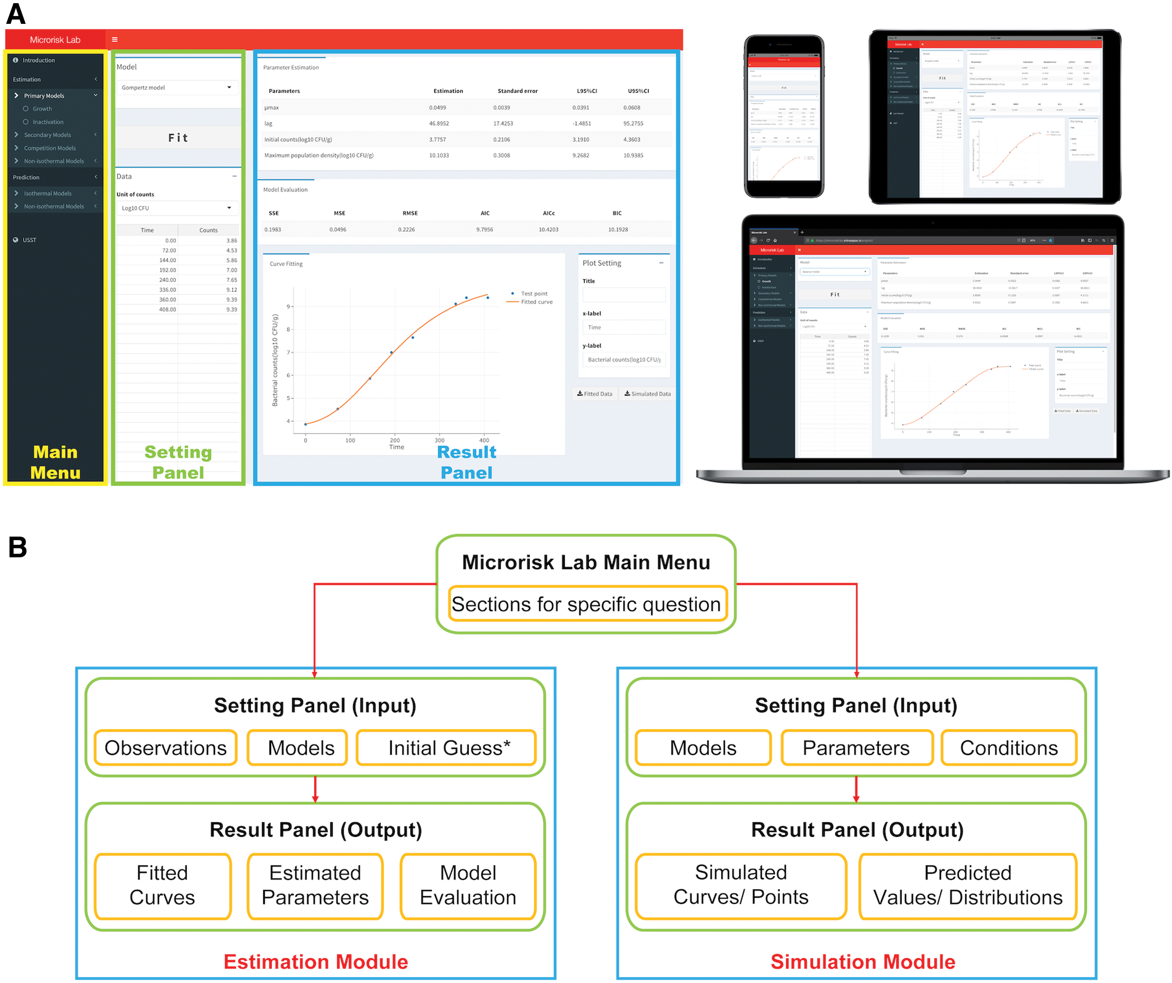
The structural framework of Microrisk Lab was divided into the “Estimation” and “Simulation” modules (Fig. 1B) for microbial kinetic analysis and simulation, respectively. In the “Estimation” module, the least-squares method was implemented to search the optimized model parameter, which was conducted by the nls function in the “stats” package. Both “NL2SOL” (for the nonisothermal analysis) and Gauss–Newton (for other analyses) algorithms were used in Microrisk Lab. In the “Simulation” module, the microbial deterministic or stochastic growth and inactivation could be simulated by defining the model type, microbial kinetic parameter, and temperature condition (or time-temperature profile). For the stochastic simulation, the probability distributions of Uniform, Normal, Lognormal, Gamma, and Logistic were performed by using the Monte Carlo method.

Mathematical models and statistical indicators

In the current version, Microrisk Lab contains 36 peer-reviewed models mentioned in most of the predictive microbiology studies implementing the microbial kinetic analysis and simulation (Supplementary Tables S1–S3). Specifically, 20 explicit equations were chosen by considering different shapes of the growth/inactivation curve for microbial dynamics under static conditions, and 10 secondary models were selected in view of the impact of temperature/pH/water activity on the specific growth rate, two piecewise functions were applied to describe two flora competition growth, and four groups of ordinary differential equations were presented by combining the primary model and secondary models for microbial growth/inactivation under nonisothermal conditions.

The second-order Runge–Kutta method or Heun's method (Press et al., 2007) was applied to solve the ordinary differential equations in the nonisothermal kinetic analysis. During the computational procedures, predicted value of the nonisothermal growth/inactivation was calculated using the Runge–Kutta method, corresponding to each of the sampling times for bacterial counting. Then, the predicted values were applied to match the observed values using a nonlinear least-squares function to determine the optimized parameter estimation. The time step (0.1, 0.01, or 0.001) was selected by the user in the regression of nonisothermal growth and inactivation.

The results of the model parameter, that is, the estimated value, standard error, and lower and upper 95% confidence intervals, were provided by the R package of “stats” and “nlstool.” Meanwhile, several statistical indicators were examined to evaluate the goodness of fit between observed and predicted values, such as the residual sum of squares (Draper and Smith, 1998), mean sum of squared error (MSE; Geeraerd et al., 2005), root MSE (RMSE; Ratkowsky, 2003), regular Akaike information criterion (AIC; Akaike, 1974), corrected AIC (AICc; Burnham and Anderson, 2003), and Bayesian information criteria (BIC; Schwarz, 1978). As pointed out by Ratkowsky (2003), the coefficient of determination (R ², Rawlings et al., 2001) and the adjusted coefficient of determination (adjusted R ², Rawlings et al., 2001) might be inappropriate for evaluating the nonlinear models. Thus, Microrisk Lab provided these two indicators only for linear models. In addition, in the stochastic simulation, the Pearson correlation coefficient was calculated to measure the linear correlation between different model variables and the final bacterial concentration, and was visualized as a tornado plot. The equations of the aforementioned indicators are listed in the Supplementary Data (Eqs. S1–S10).

Evaluation of Microrisk Lab

To evaluate the performance of Microrisk Lab, we collected six data sets (Supplementary Tables S4–S9) from the published articles and laboratory observations as six case studies: the isothermal growth of Listeria monocytogenes (Case I; Buchanan and Phillips, 1990), the isothermal inactivation of Salmonella enterica (Case II; Wang et al., 2017), the effect of temperature on the maximum specific growth rate of Salmonella Typhimurium (Case III; Oscar, 2002), the nonisothermal growth of L. monocytogenes (Case IV; unpublished data), the nonisothermal inactivation of Bacillus sporothermodurans IC4 spores (Case V; Garre et al., 2017), and the stochastic growth of S. Typhimurium individual cell (Case VI; Koutsoumanis and Lianou, 2013).

Case I–III focused on the primary and secondary modeling. Three integrated freeware and a numerical analysis system (Excel DMFit 3.5, GInaFiT 1.7, IPMP 2013, and GraphPad Prism 7.0 [GraphPad Software]) were separately applied for regression and comparison in parallel with Microrisk Lab. Case IV and V were used to introduce the availability of Microrisk Lab for nonisothermal growth and inactivation modeling. Since there were no other integrated systems specialized for the kinetic analysis of nonisothermal growth, only Bioinactivation FE (Garre et al., 2018) was applied for comparison with Microrisk Lab for the nonisothermal inactivation modeling. Case VI was a simulation example to show stochastic growth of an individual cell when considering the uncertainty and variability. The Monte Carlo simulation was performed in both Microrisk Lab and @Risk for Excel 6.0 (Palisade Corporation) for comparison.

Results

Practical examples for the primary and secondary modeling

When using Microrisk Lab for modeling, observed data or settings can be easily typed in the data dialog or pasted from other table files. If the regression is successful, the results of the parameter estimation and model evaluation are presented together with an interactive plot. Users can specify the number of significant digits and directly save the fitted curve as a local image file (Portable Network Frame file, Figs. 2 and 3), or download the generated data for replotting in other graphing systems.

FIG. 2.

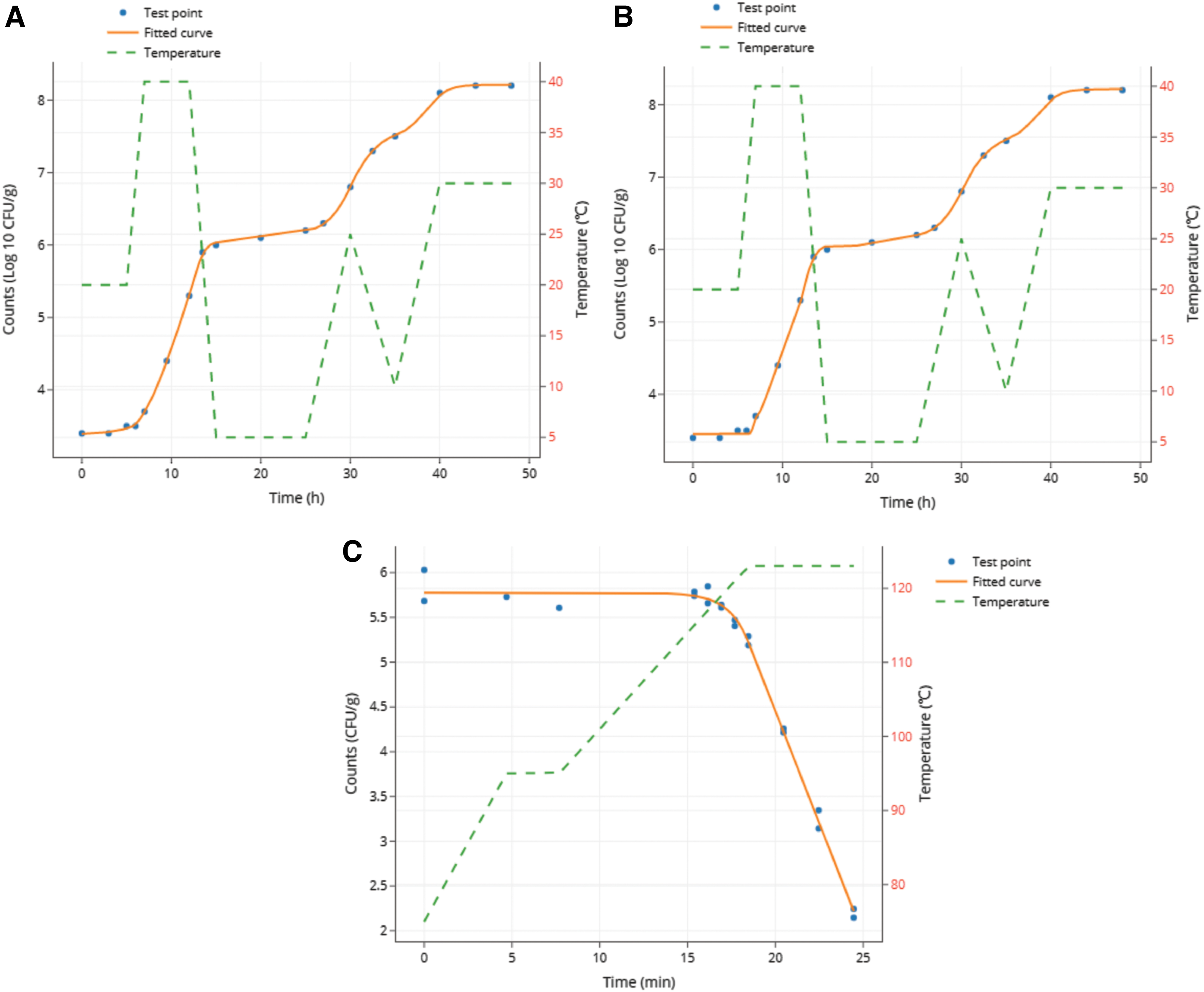
The fitted curve of (A) Case I with the “Complete Baranyi model,” (B) Case II with the “No tail Geeraerd model,” and (C) Case III with the “Cardinal parameter model” downloaded from Microrisk Lab. (The blue dot represents the observed bacterial count and the orange solid line represents the fitted curve.) Color images are available online.

FIG. 3.

The fitted curve of Case IV with (A) the Baranyi-Cardinal parameter model and (B) the Huang-Cardinal parameter model, and (C) Case V with the Dynamic Bigelow model downloaded from Microrisk Lab. (The blue dot represents the observed bacterial count, the orange solid line represents the fitted curve, and the green dash line represents the temperature profile.) Color images are available online.

The data for Case I were obtained from the ComBase browser (ComBase ID: LM127_11), based on the measurement of the growth of L. monocytogenes in tryptose phosphate broth from Buchanan and Phillips (1990). To compare with the Excel DMFit, the “Complete Baranyi model” in Microrisk Lab was chosen to determine the kinetic parameters of L. monocytogenes. Figure 2A shows the fitting curve downloaded from Microrisk Lab. Supplementary Table S10 lists the results of the estimation and evaluation in the Microrisk Lab, DMFit, and GraphPad. It should be noted that the two curvature parameters of the model need to be determined and fixed before regression in DMFit. According to the manual for Excel DMFit, the default values for the two curvature parameters are nCurv = 1 and mCurv = 0, respectively. In contrast, all estimable parameters were determined by globally searching for the optimized estimates in Microrisk Lab and GraphPad, which might have caused the discrepancy. The evaluation indicators and standard errors of the parameters became closer when increasing the value of nCurv from default 1 to 2 in Excel DMFit. Since the model evaluation indicators were different between DMFit tools and others, we further calculated the adjusted R ² according to the regression in Microrisk Lab for comparison. The results illustrate that the goodness of fit has no obvious differences between Microrisk Lab, GraphPad, and DMFit with different curvature settings.

According to the suggestion by the author of Case II, the inactivation of S. enterica in brain heart infusion under 60°C can be described by the “Log-linear + Shoulde” model in GInaFiT, which is the same as the “No-tail Geeraerd model” in Microrisk Lab (Fig. 2B). As listed in Supplementary Table S11, the results of the estimated parameters and evaluation indicators show no difference between Microrisk Lab and GInaFiT when using the same model.

Furthermore, the observed effect of temperature on the maximum specific growth rate of S. Typhimurium in chicken breast is similar in Microrisk Lab, IPMP 2013, and GraphPad by the cardinal parameters model (Supplementary Table S12 and Fig. 2C). Note that the equation of AIC built-in IPMP 2013 was referred to the study by van Boekel and Zwietering (2007), which was different from that of the built-in Microrisk Lab. The aforementioned results indicated that Microrisk Lab is as accurate as the other integrated systems for primary and secondary modeling studies.

Practical examples for the dynamic modeling

In Case IV, an unpublished study on L. monocytogenes growth in cooked beef samples under fluctuating temperatures was introduced for the nonisothermal growth modeling. During the experiments, four L. monocytogenes strains (serotypes 1/2a, 1/2b, 1/2c, and 4b; isolated from meat) were inoculated in a heat-treated ready-to-eat braised beef product (ca. 1% NaCl, pH = 6.2, a _w = 0.983) and incubated in an air-packaged sterile stomacher bag under the fluctuating temperatures between 5°C and 40°C. Both the time-temperature profile and bacterial counting data were required for the dynamic analysis. The initial hypotheses of the model parameters were required to assist in regression convergence easily. According to previous studies (ICMSF, 1996; Magalhães et al., 2014), L. monocytogenes probably has a growth temperature range of 0–45°C, with an optimal specific growth rate of ∼1 ln CFU/h (or 1/h) at 37°C in meat products. The initial hypotheses (default values) of q ₀, A, and m are preset as 1 in Microrisk Lab when there is no reliable basic knowledge of these parameters. With the aforementioned initial settings, both regressions converged successfully (Fig. 3A and B). The microbial growth parameters were obtained from Microrisk Lab with measurements under nonisothermal conditions in a single analysis. Meanwhile, the Baranyi-Cardinal parameter model and Huang-Cardinal parameter model may well describe the nonisothermal growth of L. monocytogenes in cooked beef (Supplementary Table S13).

Similarly, with the microbial enumeration data and time-temperature profile in Case V, the nonisothermal inactivation fitting could be performed using the dynamic Bigelow model in Microrisk Lab (Fig. 3C). The initial hypotheses of the estimable parameters were quoted from the primary study (Supplementary Table S14), where the referenced temperature was fixed to 120°C (Garre et al., 2017). The obtained estimations of Microrisk Lab are close to those of Bioinactivation FE (Supplementary Table S14). It should be noted, however, that different numerical analysis methods in Microrisk Lab and Bioinactivation FE might cause different truncation errors in a regression (Butcher, 2016). Thus, the evaluation indicators of AIC, AICc, and BIC provided from different modeling platforms for model comparison should be carefully examined.

Practical example for the stochastic growth simulation

The stochastic-type model can be applied to the static simulation in Microrisk Lab by defining the distribution of different model variables. As previously mentioned, the behavior of microorganisms may be quite different when the population size decreases to the single-cell level. Thus, it is necessary to consider the uncertainty and variability of cells during the simulation. In the referenced study of Case VI, Koutsoumanis and Lianou (2013) described the growth of S. Typhimurium at the different single-cell levels by establishing a stochastic model. Depending on the condition for the software of @Risk for Excel, the parameter setting of Microrisk Lab was listed in Supplementary Table S9, and the simulated results are presented in Figure 4A and B based on the Buchanan model. The probability distribution of the specific growth rate and final bacterial concentration is provided with the mean value and standard deviation in Figure 4C. According to the definition of the coefficient of variation (%CV = 100 × standard deviation/mean) in the original study, the estimated %CV for S. Typhimurium final concentration was also ∼25.5% in Microrisk Lab. The aforementioned results demonstrate that Microrisk Lab can perform a Monte Carlo simulation for bacterial stochastic modeling. Moreover, Figure 4D shows the tornado graph of the sensitivity analysis of bacterial counts obtained using different associated parameters. Thus, restricted by the aforementioned settings, the uncertainty of the duration of growth time has a relatively higher impact (than other variables) on the bacterial count during the stochastic growth of S. Typhimurium single cell.

FIG. 4.

Monte-Carlo simulation of 1 cell growth with 10, 000 iterations in (A) Microrisk Lab, and (B) @RISK for Excel (adapted from Fig. 7 of Koutsoumanis and Lianou, 2013). (C) Simulated distribution of the maximum specific growth rate and final bacterial count. (D) Tornado graph of the sensitivity analysis between model variables and bacterial counts. Color images are available online.

Discussion

In recent years, software development has become an important topic for modelers to facilitate the application of predictive microbiology (Tenenhaus-Aziza and Ellouze, 2015; González et al., 2019). Packages integrated comprehensive microbial models, such as DMFit, IPMP, and GInaFiT, significantly reduce the work burden of relevant modelers on curve fitting, parameter estimation, and model evaluation. Microrisk Lab was developed for a similar purpose, which additionally provides improvements on model options, statistical indicators, and usability. The web-based architecture allows users to access the latest version of Microrisk Lab through any internet-connected device without coding and installation.

Because a reliable tool must provide accurate results, we introduced six modeling tasks and compared them with other peer-reviewed packages to validate the availability and functionality of Microrisk Lab. Practical examples elucidated that there was no statistical difference between the results obtained from Microrisk Lab and other existing modeling systems in both regression and simulation studies.

However, the model applicability and functionality of Microrisk Lab still need to be expanded in future updates. For example, the integrated model should focus on the impact of the interaction between different intrinsic or extrinsic factors on microorganisms. The optimal model can be recommended automatically according to the input data. Regression and simulation should be developed with more algorithms, such as the Levenberg–Marquardt and adaptive Markov chain Monte Carlo algorithms provided in Bioinactivation FE (Garre et al., 2018). The Latin Hypercube sampling method should also be considered to improve the stochastic sampling efficiency (Ding et al., 2013; Membré and Boué, 2018; Dogan et al., 2019).

In summary, Microrisk Lab can be easily applied in microbial predictive modeling, especially for kinetic analysis under nonisothermal conditions. This freeware may serve as a reliable modeling tool and a useful educational resource for predictive microbiology.

Footnotes

Acknowledgment

We thank Dr. Lihan Huang in the Eastern Regional Research Center of USDA, USA, for his helpful guidance on the R programming. The preprint of this study was previously deposited in the bioRxiv server at https://www.biorxiv.org/content/10.1101/2020.07.23.218909v1.

Disclosure Statement

No competing financial interests exist.

Funding Information

This work was supported by the National Key Research and Development Program of China (Grant No. 2019YFE0103800) and the National Natural Science Foundation of China (Grant No. 12071293).

Supplementary Material

Supplementary Data

Supplementary Table S1

Supplementary Table S2

Supplementary Table S3

Supplementary Table S4

Supplementary Table S5

Supplementary Table S6

Supplementary Table S7

Supplementary Table S8

Supplementary Table S9

Supplementary Table S10

Supplementary Table S11

Supplementary Table S12

Supplementary Table S13

Supplementary Table S14

References

Akaike

. A new look at the statistical model identification. IEEE Trans Automat Contr, 1974; 19:716–723.

Alonso

, Molina

, Theodoropoulos

. Modeling bacterial population growth from stochastic single-cell dynamics. Appl Environ Microbiol, 2014; 80:5241–5253.

Augustin

J-C

. Challenges in risk assessment and predictive microbiology of foodborne spore-forming bacteria. Food Microbiol, 2011; 28:209–213.

Augustin

J-C

, Ferrier

, Hezard

, Lintz

, Stahl

. Comparison of individual-based modeling and population approaches for prediction of foodborne pathogens growth. Food Microbiol, 2015; 45:205–215.

Baranyi

, Buss da Silva

. The use of predictive models to optimize risk of decisions. Int J Food Microbiol, 2017; 240:19–23.

Baty

, Delignette-Muller

. nlsMicrobio: Nonlinear regression in predictive microbiology. R package version 0.0-1. 2015; Available at: www.r-project.org, accessed July 20, 2020 .

Buchanan

, Phillips

. Response Surface model for predicting the effects of temperature pH, sodium chloride content, sodium nitrite concentration and atmosphere on the growth of Listeria monocytogenes . J Food Protect, 1990; 53:370–376.

Burnham

, Anderson

, eds. Model Selection and Multimodel Inference. New York: Springer, 2003.

Busschaert

, Geeraerd

, Uyttendaele

, Van Impe

. Sensitivity analysis of a two-dimensional quantitative microbiological risk assessment: Keeping variability and uncertainty separated. Risk Anal, 2011; 31:1295–1307.

10.

Butcher

, ed. Numerical Methods for Ordinary Differential Equations (3rd ed.). New York: Wiley, 2016.

11.

Chang

, Borges Ribeiro

. shinydashboard: Create dashboards with ‘Shiny’. R package version 0.7.1. 2019; Available at: www.r-project.org, accessed July 20, 2020 .

12.

Cornu

, Billoir

, Bergis

, Beaufort

, Zuliani

. Modeling microbial competition in food: Application to the behavior of Listeria monocytogenes and lactic acid flora in pork meat products. Food Microbiol, 2011; 28:639–647.

13.

Ding

, Iwahori

, Kasuga

, Wang

, Forghani

, Park

M-S

, et al. Risk assessment for Listeria monocytogenes on lettuce from farm to table in Korea. Food Control, 2013; 30:190–199.

14.

Dogan

, Clarke

, Mattos

, Wang

. A quantitative microbial risk assessment model of Campylobacter in broiler chickens: Evaluating processing interventions. Food Control, 2019; 100:97–110.

15.

Dolan

, Habtegebriel

, Valdramidis

, Mishra

. Thermal processing and kinetic modeling of inactivation. In: Bakalis S, Knoerzer K, Fryer PJ, eds. Modeling Food Processing Operations. Cambridge: Woodhead Publishing, 2015, pp. 37–66.

16.

Draper

, Smith

, eds. Applied Regression Snalysis (3rd ed.). New York: Wiley, 1998.

17.

Garre

, Clemente-Carazo

, Fernández

, Lindqvist

, Egea

. Bioinactivation FE: A free web application for modelling isothermal and dynamic microbial inactivation. Food Res Int, 2018; 112:353–360.

18.

Garre

, Fernández

, Lindqvist

, Egea

. Bioinactivation: Software for modelling dynamic microbial inactivation. Food Res Int, 2017; 93:66–74.

19.

Geeraerd

, Valdramidis

, Van Impe

. GInaFiT, a freeware tool to assess non-log-linear microbial survivor curves. Int J Food Microbiol, 2005; 102:95–105.

20.

Geeraerd

, Valdramidis

, Van Impe

. Erratum to “GInaFiT, a freeware tool to assess non-log-linear microbial survivor curves”. [Int J Food Microbiol, 2005; 102:95–105]. Int J Food Microbiol 2006;102:297.

21.

González

, Possas

, Carrasco

, Valero

, Bolívar

, Posada-Izquierdo

, et al. ‘MicroHibro’: A software tool for predictive microbiology and microbial risk assessment in foods. Int J Food Microbiol, 2019; 290:226–236.

22.

Göransson

, Nilsson

, Jevinger Å. Temperature performance and food shelf-life accuracy in cold food supply chains—Insights from multiple field studies. Food Control, 2018; 86:332–341.

23.

Hamner

, Frasco

, LeDell

. Metrics: Evaluation metrics for machine learning. R package version 0.1.4. 2018; Available at: www.r-project.org, accessed July 20, 2020 .

24.

Huang

. IPMP 2013—A comprehensive data analysis tool for predictive microbiology. Int J Food Microbiol, 2014; 171:100–107.

25.

Huang

IPMP Global Fit—A one-step direct data analysis tool for predictive microbiology. Int J Food Microbiol, 2017a;262:38–48.

26.

Huang

Dynamic identification of growth and survival kinetic parameters of microorganisms in foods. Curr Opin Food Sci, 2017b;14:85–92.

27.

Hwang

C-A

, Huang

. Dynamic analysis of competitive growth of Escherichia coli O157:H7 in raw ground beef. Food Control, 2018; 93:251–259.

28.

Iannetti

, Salini

, Sperandii

, Santarelli

, Neri

, Di Marzio

, et al. Predicting the kinetics of Listeria monocytogenes and Yersinia enterocolitica under dynamic growth/death-inducing conditions, in Italian style fresh sausage. Int J Food Microbiol, 2017; 240:108–114.

29.

ICMSF (International Commission on Microbiological Specifications for Foods). Listeria monocytogenes. In: Robert TA, Baird-Parker AC, Tompkin RB eds. Microorganisms in Foods 5: Characteristics of Microbial Pathogens. London: Blackie Academic and Professional, 1996, pp. 148.

30.

Koutsoumanis

, Lianou

. Stochasticity in colonial growth dynamics of individual bacterial cells. Appl Environ Microbiol, 2013; 79:2294–2301.

31.

Koutsoumanis

, Lianou

, Gougouli

. Latest developments in foodborne pathogens modeling. Curr Opin Food Sci, 2016; 8:89–98.

32.

, Huang

, Yuan

. Growth and survival of Salmonella Paratyphi A in roasted marinated chicken during refrigerated storage: Effect of temperature abuse and computer simulation for cold chain management. Food Control, 2017; 74:17–24.

33.

Magalhães

, Mena

, Ferreira

, Silva

, Almeida

, Gibbs

, Teixeira

. Listeria monocytogenes. In: Motarjemi Y, Moy G, Todd E, eds. Encyclopedia of Food Safety. Oxford: Elsevier, 2014, pp. 450–461.

34.

Membré

J-M

, Boué

. Quantitative microbiological risk assessment in food industry: Theory and practical application. Food Res Int, 2018; 106:1132–1139.

35.

Ndraha

, Hsiao

H-I

, Vlajic

, Yang

M-F

, Lin

H-TV

. Time-temperature abuse in the food cold chain: Review of issues, challenges, and recommendations. Food Control, 2018; 89:12–21.

36.

Oscar

. Development and validation of a tertiary simulation model for predicting the potential growth of Salmonella typhimurium on cooked chicken. Int J Food Microbiol, 2002; 76:177–190.

37.

Peleg

, Corradini

. Microbial growth curves: What the models tell us and what they cannot. Crit Rev Food Sci Nutr, 2011; 51:917–945.

38.

Plaza-Rodriguez

, Thoens

, Falenski

, Weiser

, Appel

, Kaesbohrer

, et al. A strategy to establish food safety model repositories. Int J Food Microbiol, 2015; 204:81–90.

39.

Pouillot

, Delignette-Muller

, Denis

. mc2d: Tools for two-dimensional Monte-Carlo simulations. R package version 0.1-18. 2017. Available at: www.r-project.org, accessed July 20, 2020 .

40.

Press

, Teukolsky

, Vetterling

, Flannery

, eds. Numerical Recipes-the Art of Scientific Computing. Cambridge: Cambridge University Press, 2007.

41.

Psomas

, Nychas

G-J

, Haroutounian

, Skandamis

. Development and validation of a tertiary simulation model for predicting the growth of the food microorganisms under dynamic and static temperature conditions. Comput Electron Agr, 2011; 76:119–129.

42.

Ratkowsky

. Model fitting and uncertainty. In: McKellar R, Lu X, eds. Modeling Microbial Responses in Foods. Boca Raton: CRC Press, 2003, pp. 151–196.

43.

Rawlings

, Pantula

, Dickey

, eds. Applied Regression Analysis: A Research Tool. New York: Springer, 2001.

44.

Ross

, McMeekin

. Predictive microbiology. Int J Food Microbiol, 1994; 23:241–264.

45.

Schwarz

. Estimating the dimension of a model. Ann Stat, 1978; 6:461–464.

46.

Tenenhaus-Aziza

, Ellouze

. Software for predictive microbiology and risk assessment: A description and comparison of tools presented at the ICPMF8 Software Fair. Food Microbiol, 2015; 45:290–299.

47.

USDA (U.S. Department of Agriculture). Pathogen Modeling Program. 2016. Available at: https://www.ars.usda.gov/northeast-area/wyndmoor-pa/eastern-regional-research-center/residue-chemistry-and-predictive-microbiology-research/docs/pathogen-modeling-program/, accessed May 1, 2018 .

48.

USDA. IPMP Dynamic Prediction. 2017. Available at: https://www.ars.usda.gov/northeast-area/wyndmoor-pa/eastern-regional-research-center/docs/ipmp-dynamic-prediction/, accessed May 1, 2018 .

49.

van Boekel

, Zwietering

. Experimental design, data processing and model fitting in predictive microbiology. In: Brul S, van Gerwen S, Zwietering M, eds. Modeling Microorganisms in Food. Cambridge: Woodhead Publishing, 2007, p. 38.

50.

Wang

, Devlieghere

, Geeraerd

, Uyttendaele

. Thermal inactivation and sublethal injury kinetics of Salmonella enterica and Listeria monocytogenes in broth versus agar surface. Int J Food Microbiol, 2017; 243:70–77.

51.

Whiting

, Buchanan

. A classification of models in predictive microbiology. Food Microbiol, 1993; 10:175–177.

52.

Wickham

, Chang

, Henry

, Pedersen

, Takahashi

, Wilke

, Woo

. ggplot2: Create elegant data visualisations using the grammar of graphics. R package version 3.1.1. 2019. Available at: www.r-project.org, accessed July 20, 2020 .

Supplementary Material

Please find the following supplemental material available below.

For Open Access articles published under a Creative Commons License, all supplemental material carries the same license as the article it is associated with.

For non-Open Access articles published, all supplemental material carries a non-exclusive license, and permission requests for re-use of supplemental material or any part of supplemental material shall be sent directly to the copyright owner as specified in the copyright notice associated with the article.

0.00 MB

0.07 MB