A Bayesian Method for Exposure Prevalence Comparison During Foodborne Disease Outbreak Investigations

Background

The Centers for Disease Control and Prevention (CDC) and state and local health departments investigate multistate foodborne disease outbreaks of salmonellosis, Shiga toxin–producing Escherichia coli infection, listeriosis, and campylobacteriosis by identifying genetically linked clusters of bacterial isolates from patients. Isolates are submitted by clinical laboratories to public health laboratories that participate in PulseNet, the national molecular subtyping network for enteric bacteria (Tolar et al., 2019). Once an illness cluster has been identified, state and local health departments conduct case-patient interviews and collect information on food exposures during the week before illness onset.

Generating hypotheses about suspect food vehicles and further investigating them is a crucial component of foodborne disease outbreak investigations. This process considers known vehicle–pathogen associations, case characteristics (e.g., demographics), and exposure information (White et al., 2021). Iteratively collecting and analyzing exposure information from cases are necessary for hypothesis generation and subsequent investigations to confirm or refute those hypotheses. Public health agencies sometimes conduct case–control studies for foodborne disease outbreaks to identify food items associated with case status. Recruitment of controls is resource intensive and time consuming, and often not feasible during a rapidly evolving outbreak investigation where timely intervention is important.

A frequently used alternative is to compare the prevalence of food item consumption among outbreak cases with the corresponding prevalence in the general population, as estimated from a sample survey (Jervis et al., 2019). CDC and many state and local health jurisdictions use the FoodNet Population Survey for this purpose. Outbreak investigators typically calculate a frequentist one-sample p-value based on the binomial probability of n or more cases reporting consumption of a particular food item, assuming the null hypothesis that the prevalence of reported consumption of cases is the same as that point estimate of the prevalence in general population from the survey (Jervis et al., 2019).

Since investigations are dynamic, this process can be repeated during an investigation as more exposure information is collected and more cases are reported. Multiple hypotheses might also be tested. A statistically significant p-value is interpreted as adding support for a particular vehicle hypothesis.

However, this method has several issues. As widely discussed in the literature on p-values and null hypothesis significance testing, the 0.05 threshold is arbitrary; a statistically significant p-value does not account for the effect size (i.e., magnitude of prevalence difference), and p-values can be easily misinterpreted. Multiple testing and the lack of a prespecified analysis plan increase Type I error and yield unreliable p-values (Greenland et al., 2016). This hypothesis testing procedure also ignores uncertainty associated with the population survey prevalence estimate.

We propose a Bayesian approach to exposure prevalence estimation among outbreak cases and comparison with the general population.

Materials and Methods

We obtained reported food consumption data for a 2020 E. coli O157:H7 illness outbreak linked to leafy greens from CDC's multistate foodborne outbreak surveillance system. Forty patients infected with the outbreak strain were reported from 19 states. Illness onset dates ranged from August 10, 2020, to October 31, 2020. Based on exposure information and historical outbreaks linked to this strain, investigators concluded that leafy greens (i.e., vegetables whose leaves are eaten, often fresh and uncooked) were the likely source of this outbreak. However, a specific type or brand could not be identified during traceback efforts. We included prospectively collected exposure data in the analysis (Centers for Disease Control and Prevention, 2020).

We included food consumption data from the 2018–2019 FoodNet Population Survey. The population survey was a complex sample survey of the catchment area population of FoodNet, an active surveillance system for foodborne bacterial infections (Centers for Disease Control and Prevention, 2021). Respondents residing in Connecticut, Georgia, Maryland, Minnesota, New Mexico, Oregon, Tennessee, and select counties in California, Colorado, and New York were randomly selected to participate.

The survey was conducted between late December 2017 through July 2019. Sampling was conducted by random digit dialing through landline phones and cell phones (24%) and by address (76%). Telephone participants completed surveys through computer-assisted telephone interview, whereas participants sampled by address completed surveys online. One participant from each household was sampled with oversampling of children (80% of selected households). Participants were asked questions about food, animal, recreational water, and travel-related exposures in the 7 days before the interview.

Respondents with incomplete questionnaires or partial responses were excluded from the analysis. Prevalence estimates and 95% confidence intervals were generated using weighted generalized estimating equations to account for the survey design and survey mode effects (Centers for Disease Control and Prevention, 2022). We included data on consumption of beef, carrots, leafy greens (defined on the questionnaire as “leafy greens such as lettuce, spinach, or kale such as in a salad, on a sandwich or burger”), iceberg lettuce, romaine lettuce, and spinach.

We simulated prospective use of the typical method and our proposed method by estimating posterior distributions of food item consumption prevalence among case-patients for one or more food items at multiple points during the investigation. We calculated the exact binomial test p-value in the usual manner. We determined a posterior beta distribution from a noninformative (flat) Beta(1,1) prior and a binomial likelihood parameterized by the number of case-patients reporting consumption of a specific food item and the total number of reported cases with food consumption information.

We estimated beta distributions for the FoodNet Population Survey prevalence estimates using the method of moments based on the reported point estimate and standard deviation of the estimate. We sampled from each distribution 100,000 times. For each sample, we subtracted the population survey prevalence estimate from the outbreak prevalence estimate. We then calculated the probability that the prevalence difference was >0, that is, that the exposure prevalence among outbreak case-patients was higher than that of the general population.

We graphed the prevalence difference distribution for each food item at each time point during the investigation. Analyses were performed in R Statistical Software (v4.0.3; R Core Team, 2020). An R script with instructions for use is included in Supplementary Appendix SA1. CDC has also made this method available to state health departments as a point-and-click tool in SEDRIC, CDC's cloud-based collaboration platform for foodborne outbreak response. This activity was reviewed by CDC and was conducted consistent with applicable federal law and CDC policy.

Results

Exposure information from three time points during the 2020 E. coli O157:H7 outbreak investigation was included in the analysis (Table 1). Initially, six patients with genetically related E. coli O157:H7 isolates were identified. Four of these six patients were successfully interviewed and reported consuming leafy greens (unspecified type), iceberg lettuce, spinach, beef, and carrots in the week before illness onset. Romaine lettuce consumption was not reported by any patients. Figure 1 displays prevalence difference distributions for each of these food items at each time point during the investigation.

OPEN IN VIEWER

FIG. 1.

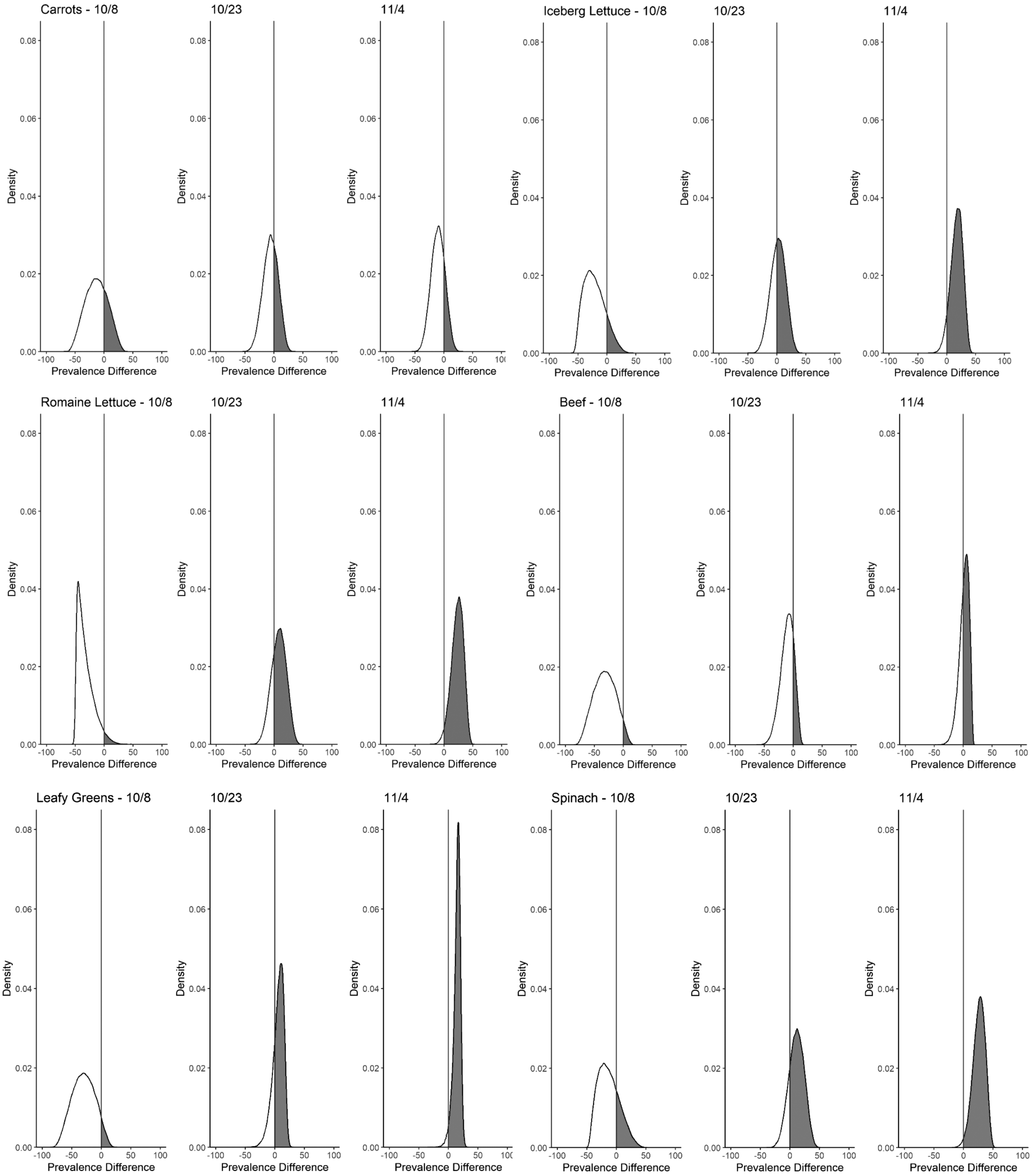
Estimated difference in food item exposure prevalence among outbreak case-patients and the 2018–2019 FoodNet Population Survey in a 2020 Escherichia coli O157:H7 outbreak by food item and date. The gray line indicates no difference in prevalence.

The probabilities for the exposure prevalence among cases being higher than that among FoodNet Population Survey participants were highest for carrots (0.27), followed by spinach (0.25), followed by iceberg lettuce (0.13), leafy greens [unspecified type] (0.06), beef (0.04), and romaine lettuce (0.03) (Table 1).

Exposure prevalence was recalculated on October 23, 2020, and exposure information was available for 12 of 22 reported cases. The probabilities were highest for spinach (0.81), followed by leafy greens [unspecified type] (0.74), romaine lettuce (0.73), iceberg lettuce (0.57), carrots (0.35), and beef (0.19). Exposure information was available for 16 of 34 cases on November 4, 2020. The probabilities were highest for spinach (0.99), followed by romaine lettuce (0.98), leafy greens [unspecified type] (0.97), iceberg lettuce (0.94), beef (0.61), and carrots (0.21). Significant exact binomial test p-values were obtained only for 2 food items (romaine lettuce and spinach) and only once 34 cases had accumulated by November 4, 2020 (Table 1).

Discussion

Estimating a posterior distribution for exposure prevalence among cases and comparing it with a population reference is a feasible alternative to the one-sample binomial test often used during foodborne outbreak investigation. This approach directly addresses the question of interest: is exposure prevalence among cases higher than the general population? Exposure prevalence comparison provides rapid and interpretable quantitative information about the relative importance of exposures reported by case-patients. It also avoids some pitfalls of frequentist null hypothesis significance testing.

Graphing and comparing prevalence difference distributions over time also illustrate change in uncertainty associated with the prevalence estimates. When applied to prospectively collected exposure data from the 2020 E. coli O157:H7 outbreak described above, the probabilities of consumption prevalence of multiple leafy green items being higher than that of the general population increased as additional case-patients were interviewed.

By October 23, 2020, probabilities that exposure prevalence was higher among case-patients as compared with the population survey were notable for leafy greens (0.74), romaine lettuce (0.73), and spinach (0.81). This occurred 2 weeks before any exact binomial p-value was significant despite the potential loss of power from appropriately considering the uncertainty in the general population estimate. Prospective use of this method will help determine the situations in which earlier evidence favoring a suspect vehicle will be most beneficial in averting subsequent cases.

Alternative Bayesian approaches to hypothesis testing might also be suitable for foodborne outbreaks. The Bayes Factor is the ratio of the likelihoods and priors under an alternative and null hypothesis (van Ravenzwaaij et al., 2019). However, it can be challenging to interpret and is unfamiliar to most applied epidemiologists. It might also encourage the use of a threshold to define a meaningfully large value. A continuous measure, as outputted in our method, is more conducive to serial weighing of evidence in support of or against a particular vehicle hypothesis.

The Region-of-Practical-Equivalence approach is another alternative in which a range of values corresponding to a null effect is defined and compared with the credible interval of a parameter of interest (Kruschke and Liddell, 2018). This dichotomizes the comparison process and provides less information than the approach we outline.

Our approach could also be extended through other Bayesian techniques. For example, using informative priors (e.g., based on known vehicle–strain associations or on the presence of highly genetically related animal or environmental isolates) might increase power to detect a difference in exposure prevalence, but choosing a prior is a complex decision and could introduce bias. Although we treated the reference and outbreak samples as independent across food exposures, this is unlikely to be true. Thus, estimating a joint posterior distribution accounting for the correlation among foods could allow for additional insights.

However, this would require access to data beyond that available from the publicly accessible FoodNet Population Survey tools. Future studies could help determine scenarios wherein more complex approaches provide benefit.

Our method does not address key issues with exposure prevalence comparison. Comparisons between the survey sample and case-patients might be biased if the survey sample does not represent the exposure distribution of the source population as in control selection bias in case-control studies (Rothman et al., 2008). Although adjustment for factors associated with selection might partially mitigate this bias, the source population is not easily defined in multistate foodborne disease outbreaks. Restricting the reference sample to match the demographic characteristics of outbreak case-patients might be another strategy to approximate the source population.

Our method also does not adjust for potential confounding; due to dietary patterns, food item consumption is highly correlated (e.g., patients who ate romaine lettuce are more likely to eat spinach than patients who did not consume romaine lettuce). As in our example, exposure information is often unavailable for all case-patients. Missingness would result in underestimated exposure prevalence among cases, and the estimated prevalence would be a minimum value. Exposure status might also be misclassified.

Finally, our method ignores possible correlation in reported exposures between case-patients, for example, when patients are members of the same household, and results in underestimation of the uncertainty of the exposure prevalence among case-patients. Bounding some of these biases might be possible and merits further exploration. Effect sizes in foodborne outbreaks are often large, and the relative magnitude of these biases might not meaningfully affect inference.

Conclusions

Exposure prevalence estimation and comparison is a useful rapid tool for generating and testing hypotheses about vehicles in foodborne disease outbreaks. The Bayesian approach we outline is an effective method to facilitate foodborne outbreak vehicle hypothesis generation and testing. Hypothesis generation and testing can lead to faster identification of a culprit food item by speeding up the timeline for key public health actions including reinterviewing patients, case–control studies, traceback, laboratory testing, and product recalls, potentially averting additional illnesses.