




Abstract
The U.S. casino industry has been considered by some to be “recession proof.” Although consumer spending has not seemed to decline dramatically during past recessions, still, the casino industry is sensitive to macroeconomic changes. In this article we examine a variety of U.S. macroeconomic indicators to determine which are most closely related to U.S. casino revenues. We find that the best predictors of U.S. casino revenues are projected gross domestic product (GDP) and personal consumption expenditures (PCE). We use our model to forecast casino revenue growth rates for 2023 through 2027.
I. INTRODUCTION
Changes in the U.S. economy have different impacts on different industries. Largely, this is due to how macroeconomic changes affect consumer expenditures on different types of goods and services. These effects can be especially complex during difficult economic times, such as over the last few years where there have been simultaneous, complicating economic and social factors, including the carryover of the COVID pandemic, the Russia/Ukraine war, high inflation (including high gas prices), a potential recession, supply chain issues, and a labor shortage.
In this article, we examine the relationship between the overall U.S. economy and consumer spending, with particular attention to consumer spending on the U.S. casino sector—including both commercial and tribal casinos. Using statistical analysis of this historical relationship, including during past economic downturns, we identify leading and lag indicators of consumer spending at U.S. casinos. We also use our best statistical model to forecast consumer spending on casino gaming in the future.
This article is organized as follows. Section II provides background on the U.S. economy and the U.S. casino sector. Section III discusses economic theory behind how macroeconomic variables are expected to affect the U.S. casino sector. Section IV provides a review of relevant academic literature to determine if there is any previously conducted research and analysis that may supplement general economic theory covered in Section III. Section V describes the data used in our analysis. The results are presented in Section VI. Section VII provides conclusions and insights for future research.
II. BACKGROUND
In order to better understand the relationship between business cycles in the U.S. economy and the U.S. casino sector, it is important to develop background on both. In this section, we provide a brief overview of the U.S. economy (section A), recent trends in the economy (B), and the casino sector (C).
A. U.S. economy
The United States economy is the largest in the world, with about $25.5 trillion in output in 2022. 1 The federal government keeps track of a large number of economic variables, but gross domestic product (GDP) and unemployment are most commonly used to track the “health” of the economy. This is because particular changes in these variables are typically the hallmarks of recessions. Economists also track fiscal variables, such as government spending and taxes, and monetary variables, such as money supply and interest rates, to understand how government reacts to macroeconomic fluctuations and how these fluctuations respond to government macroeconomic policies.
GDP measures the value of goods and services produced in an economy during a particular year. GDP, and various other measures that can be derived from it, can be compared across countries and through time in order to assess productivity. For example, China is the world's second largest economy, with 2022 GDP of US $18.0 trillion. 2 GDP is also a good measure for understanding how different events, such as a worldwide shock like the COVID-19 pandemic, affected different countries. When GDP and other variables are compared over longer periods of time, it is common to adjust the data for inflation (changes in the value or purchasing power of the dollar). The unadjusted values are referred to as “nominal” (e.g., nominal GDP), while the adjusted values are referred to as “real” (e.g., real GDP).
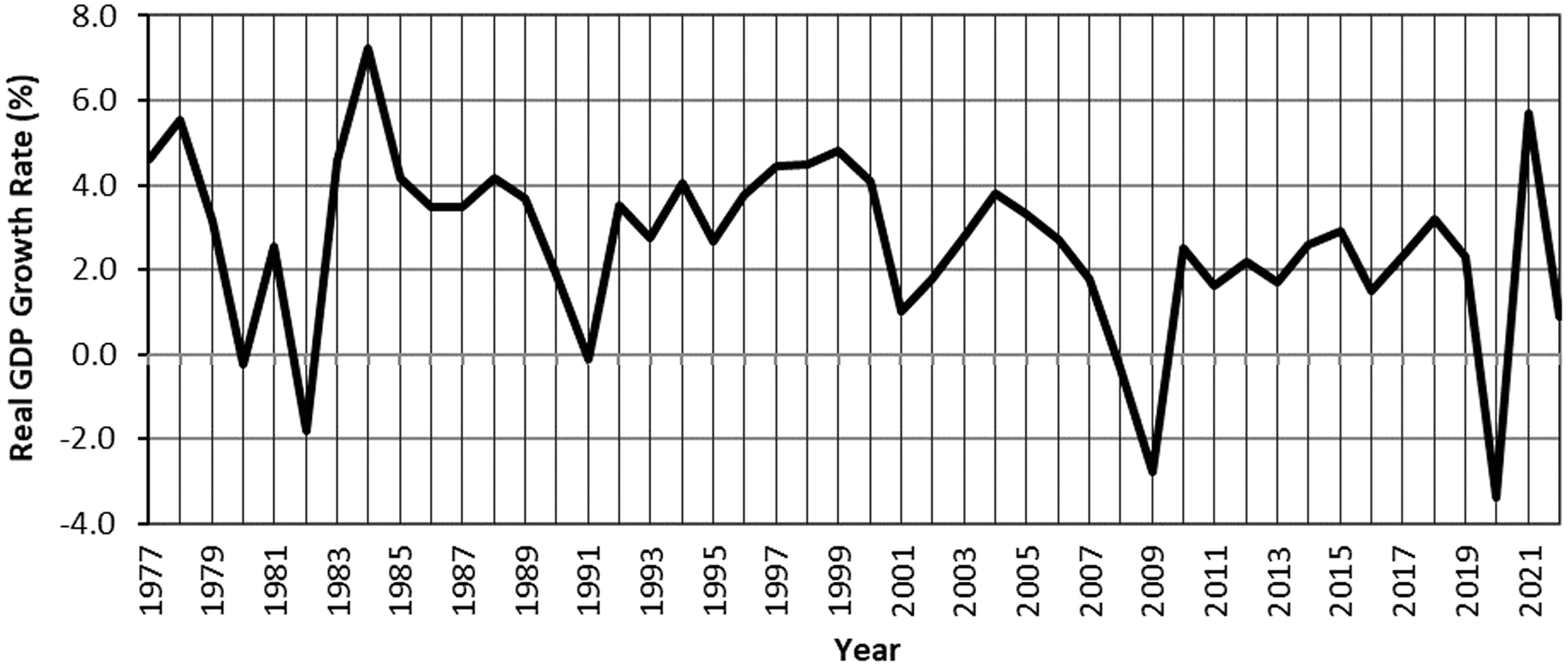
Fig. 1 illustrates the U.S. annual real GDP growth rate from 1977–2022. As can be seen in the figure, the highest growth rate was around 7% in 1984; the lowest was during the COVID-19 pandemic in 2020, with -3% annual growth. During the period shown in the graph, the average growth rate was 2.6%. Economists informally define a “recession” as two or more consecutive quarters (i.e., at least six months) of negative economic growth, however, the dates of entry and exit from recession are formally determined by the National Bureau of Economic Research (NBER) based on a longer list of macroeconomic variables.
Real Growth Rate of U.S. GDP, 1977–2022. Source: U.S. Bureau of Economic Analysis
Since 1977, there have been six officially recognized recessions: 1980, 1981–1982, 1990–1991, 2001, 2007–2009, and 2020. Even though Fig. 1 plots annual data, the recessions are clearly indicated by the negative growth rates during those years. 3 When real GDP growth rate is negative (i.e., during recessions), it means the level of production (or output) in the U.S. economy is declining. Because negative real GDP growth reflects decreasing production, we should also expect fewer people to be employed. For this reason, when real GDP is falling or experiencing negative growth, economists typically expect the unemployment rate will be rising.
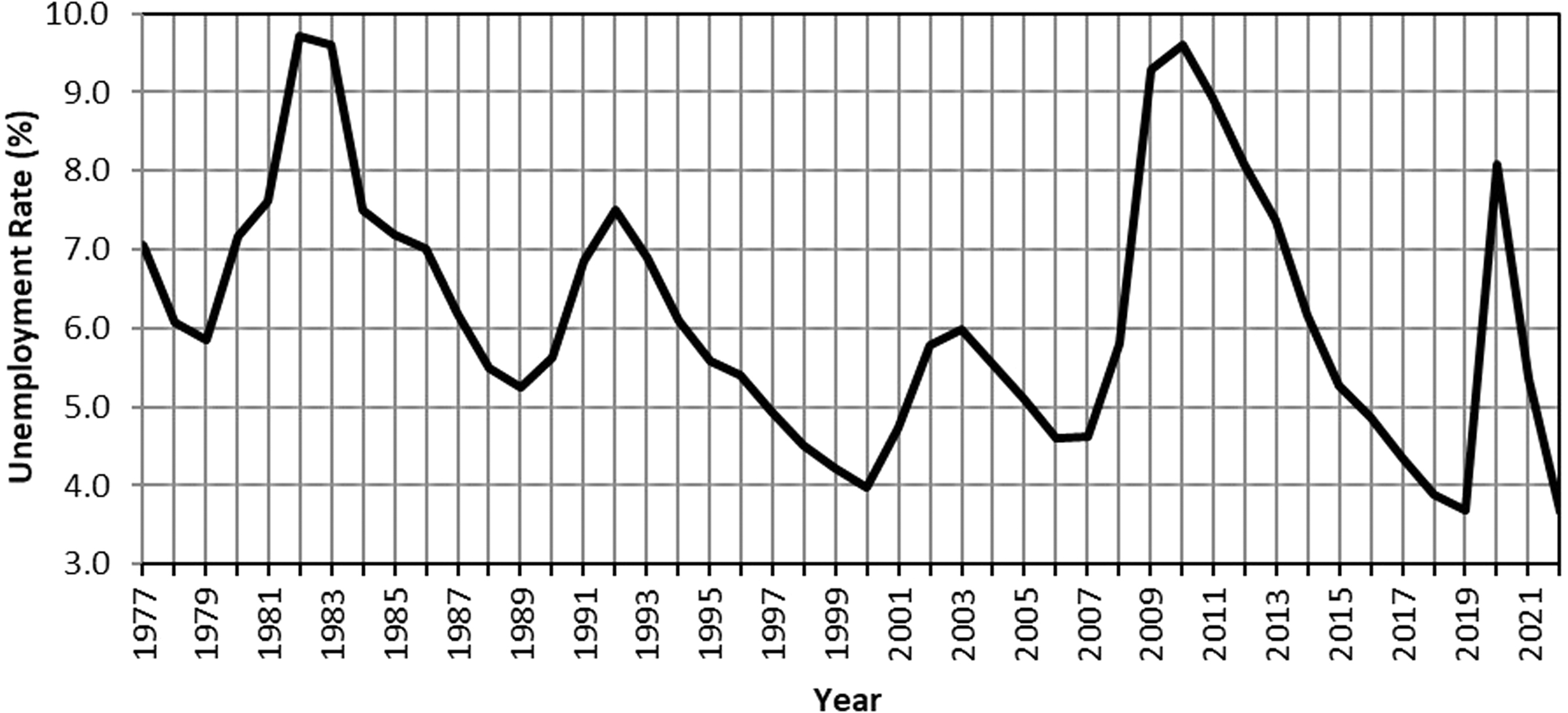
The unemployment rate is the percentage of people in the labor force (employed people + people seeking jobs) who are unemployed. Fig. 2 illustrates the annual average unemployment rate. It is clear from the figure that the unemployment rate has increased around each of the recessions illustrated in Fig. 1. Comparing Figs. 1 and 2, we can see that the troughs in GDP growth are fairly consistent with the peaks of unemployment. However, they do not follow each other perfectly. For example, notice that in the recovery from the 1991 recession, GDP was growing at 3.5% in 1992, while unemployment peaked in 1992 at 7.5%. Thus, even though these variables are related and tend to move together, albeit in opposite directions in this case, there are often differences in the exact timing (leads and lags).
U.S. Unemployment Rate, 1977–2022. Source: U.S. Bureau of Labor Statistics
Closely related to the unemployment rate is the labor force participation rate (LFPR), which is the number of people in the labor force (employed people + people seeking jobs) as a percentage of the civilian population. Fig. 3 shows the labor force participation rate. Although the labor force participation rate has been fairly constant from 2014 through 2019, a decrease can be noticed starting at the onset of the COVID-19 pandemic. In late 2020 and during 2021, a significant number of people left the labor force as a result of closures and layoffs during the pandemic, older workers leaving the work force to avoid health risks, and a significant number of two-worker households decreasing to one worker. This was described in the media as the “great resignation.” Notably, because of the fairly stable historical level in the LFPR, other macroeconomic variables are better indicators of the short-term business cycle fluctuations experienced in the economy.

U.S. Labor Force Participation Rate, 1977–2022. Source: U.S. Bureau of Labor Statistics
Recessions affect industries differently. For example, we might expect the market for new cars to see a large decrease in demand during a recession, presumably because less people have jobs and those that do are likely to be more restrictive in their spending. The same might occur in the tourism market. People are less likely to plan cruises or ski vacations during a recession given incomes are expected to decrease. However, the demand in markets for other goods such as toilet paper or eggs is not likely to suffer as large of a decline during a recession. The recent recession associated with the COVID-19 pandemic obviously affected travel and tourism related industries differently than other recessions due to the unprecedented government-imposed travel bans and shutdowns. Some commentators have historically argued that the casino sector is “recession proof,” a claim we will discuss in more detail in the literature review below (Section IV).
B. Current economic conditions
The U.S. economy is still considered to be recovering from the shock of the COVID-19 pandemic and related government policy changes, especially in monetary policy. Shutdowns throughout the economy in Spring 2020 at the beginning of the pandemic, along with significant increases in government spending and the money supply in response to the pandemic, represented real shocks to the economy. Federal government spending in 2019 was $4.88 trillion but increased to between $6.2 and $7.3 trillion from 2020 to 2022. 4 The Federal Reserve (Fed) also rapidly expanded the supply of money in the U.S. economy by 44% from February 2020 to April 2022. 5
Increases in government spending and the money supply of this magnitude, in combination with shutdowns across the economy and supply chain issues, inevitably led to higher inflation, as more money is chasing fewer goods and services. In addition, Russia's invasion of Ukraine has contributed to higher prices of gas and other goods, further exacerbating inflation. The annual inflation rate rose to a high of just over 9% in June 2022.
In an effort to lower inflation, the Fed has been reducing the money supply and increasing interest rates. The Fed increased the federal funds target rate 11 times from March 2022 through July 2023, up from 0%–0.25% at the beginning of the pandemic (i.e., March 2020) to its current level of 5.25%–5.5% in July 2023. 6 These repeated increases were intended to decrease spending in the economy. Since June 2022, the inflation rate has started falling, and stood at 3.7% as of September 2023. 7
It is difficult to predict how the economy will grow in the near future given the complicated factors. Many economists predict a mild recession due to the higher interest rates set by the Fed to combat inflation. Despite some months of negative economic growth in 2022, there was no official recession. However, some economists are still predicting one will begin by early 2024.
C. U.S. casino sector
The U.S. gaming industry consists of a variety of uniquely operated and regulated sectors, including casinos, lotteries, card rooms, pari-mutuel wagering, charitable gaming, convenience gambling (i.e., non-tribal restaurants, bars, taverns, drugstores, and other retail businesses with stand-alone gaming machines), and internet/online gaming.
The largest sector, by far, is casinos. It consists of brick-and-mortar facilities in which consumers gamble in person on games of chance. The facilities can offer a wide array of games, including gaming machines, table games, poker, keno, bingo, and sports betting. There are a few different types of casinos: commercial land-based, racetrack, and riverboat casinos, and Indian gaming facilities:
▪ Commercial casinos are traditional casinos commercially operated under state gaming laws (e.g., Las Vegas and Atlantic City). Commercial casinos include land-based casinos, riverboat/dockside casinos, and limited-stakes casinos. ▪ Racetrack casinos (“racinos”) are the portion of racetracks allowed to commercially operate casino games under state gaming laws. ▪ Indian gaming facilities include any tribally operated enterprise that offers Class II or Class III gaming in accordance with the Indian Gaming Regulatory Act (IGRA). Thus, Indian gaming facilities may include casinos, bingo halls, travel centers, gas stations, tobacco shops, convenience stores, restaurants, and bars. Indian gaming facilities do not include gaming facilities operated by tribes under state laws and regulations rather than IGRA.
Nevada was the first state to legalize casinos in 1931. It was the only state in which legal casinos operated until 1978, when casinos began operating in Atlantic City, New Jersey. There was no further geographic expansion of casinos until the U.S. Supreme Court's 1987 decision in California v. Cabazon Band of Mission Indians. 8 The Court ruled that the State of California did not have the authority to enforce its gambling laws on Indian lands given that the State permitted a substantial amount of gambling activity and even promoted gambling through the state lottery. However, this decision increased tensions between tribes and states and fueled lobbying efforts for federal legislation to govern Indian gaming. 9 Finally, as a compromise between tribal and state interests, Congress passed the Indian Gaming Regulatory Act (IGRA) in 1988 to regulate the conduct of gaming on Indian lands and establish a regulatory structure for Indian gaming in the United States. 10
For Class III Indian gaming (e.g., slot machines and banked table games), IGRA also requires tribes to negotiate a gaming compact with the state in which they are located. Per IGRA and these compacts, regulatory powers over Class III Indian gaming are shared by the federal government, the tribe that operates gaming, and the state in which the gaming is located. While IGRA expressly prohibits states from imposing any tax, fee, charge, or other assessment upon a tribe as a condition to operate gaming facilities under federal law, 11 many tribes make direct gaming-related payments, such as reimbursements of regulatory costs; 12 local revenue sharing; 13 and state revenue sharing. 14 However, as sovereign nations, tribes are not required to make payments other than regulatory cost reimbursements in order to operate gaming—they do so voluntarily.
As politicians began negotiating compact agreements with tribes, some state governments decided to host commercial casinos. 15 The stated purpose of legalizing commercial casinos in the 1990s was often to attract tourists, raise tax revenue, and stimulate economic growth and employment in the hosting state. In effect, casinos legalization was seen as a sort of state-level fiscal policy. During the 1990s, eight states, most of which bordered the Mississippi River, began hosting commercial riverboat/dockside casinos. Beyond the mid-1990s, new states legalized casinos at a slower pace. But a host of new states legalized casinos over time.
As of the end of 2022, the U.S. hosted 352 land-based casinos, 66 riverboat casinos, 50 racinos, and 523 tribal casinos across 42 states. 16 As noted above, the casino sector is the largest in the U.S. gaming industry, and most of its growth has occurred only in the last 30 years.
Other types of gambling began developing later, as casinos expanded, regulations were relaxed, and technology developed. The most recent forms of legal gambling include online gaming, including poker, casinos games, and lotteries, as well as mobile gambling (i.e., gambling on a mobile device). Online gaming revenue increased dramatically during the COVID-19 pandemic, and in the six states it is legal, total revenues exceeded $5 billion in 2022. 17
The widespread legalization of sports betting outside of Nevada began after the 2018 Supreme Court decision in Murphy v. National Collegiate Athletic Association, 18 which struck down the 1992 Professional and Amateur Sports Protection Act (PASPA). By the end of 2022, 33 states had legalized sports betting. 19 States vary in terms of whether they allow sports betting only at brick-and-mortar casinos, and/or online within the state.
III. ECONOMIC THEORY
In the previous section, we examined different macroeconomic variables that help give a picture of how the U.S. macroeconomy is performing. We also briefly discussed the development of the casino sector in the U.S. Using this as context, in Section III-A, we develop a simple model of the macroeconomy in order to decipher which macro variables may best be associated with the performance of the casino sector as a whole. In Section III-B we discuss some economic and social factors that affect the U.S. economy's recent performance.
A. Model of the macroeconomy
Macroeconomic theory is a field that is constantly changing as new data become available over time. However, one model in particular is probably best suited to use in this article to get a better understanding of how the macroeconomy works. The Keynesian model, developed in the 1930s and refined in the following decades, provides the framework we explain in this section. 20 We keep the discussion general in order to avoid unnecessary technicalities that would add little to the discussion.
As a starting point, it is important to note that the total expenditures in an economy will equal total income. This is true because when a person buys a new car, what the customer spends, the car dealer receives (i.e., income=expenditure). It follows, for reasons we will discuss below, that the total value of production in the economy (GDP) is equal to “national income” (we abbreviate it as Y), which must equal total expenditures. Thus, we have the following equation for GDP:
Our goal in this article is to better understand how consumer spending in particular may be related to revenues in the casino sector. Therefore, it is helpful to partition total spending/revenue into several different sources. The following equation illustrates the classic macroeconomic model we discuss in the rest of this section. The equation shows that GDP, or total income (Y), is composed of several components, namely consumption spending (C), investment (I), government spending (G), and net exports (NX).
Consumption spending (C) includes goods and services purchased by individuals within the economy. This includes spending on food, clothing, cars, computers, and all other “final” goods and services. This would include money spent at casinos and on all other forms of gambling.
Investment (I) includes private domestic investment and capital expenditures by businesses. Investment includes spending on machinery, vehicles, and buildings, as well as the value of houses built during the year. 21
Government spending (G) refers to the purchase of goods and services at various levels of government (i.e., city, state, and federal). A significant amount of government spending is transfer payments, such as Social Security, which are excluded from G given such spending does not involve the purchase of goods and services produced in the economy. 22 This money is counted when recipients of the transfer payments spend the money on consumption or investment.
Finally, net exports (NX) are the value of products exported (E) from the U.S. to other countries, minus the value of products imported (M) from other countries, so that NX=E - M. Products that are exported from the U.S. are a component of U.S. production and should be included in GDP. However, imports are products consumed here but produced elsewhere, so they are subtracted from the GDP measure.
As shown in Equation (2), GDP increases when any one component (C, I, G, or NX) increases. In order to better understand the determinants of GDP, we can specify variables that directly affect C and I, and therefore indirectly affect GDP.
Consumers' spending on goods and services (C) will be affected by their after-tax income and interest rates. If taxes increase, consumers will have less money left over for spending. If interest rates rise, it makes saving relatively more attractive than before, and we would expect consumption to decrease. Investment spending by businesses (I) is similar. If business taxes increase, businesses would be expected to decrease their purchases simply because they have less money. As interest rates increase, businesses are less likely to take loans to buy equipment, expand factories, and so on.
There are no specific determinants of G, as government spending is set through a political process, but this is where any expansionary fiscal policy expenditures would be reflected. Net exports (NX) are affected by factors such as exchange rates, which are not particularly relevant to the subject in this article. We focus instead on I, and especially C.
B. U.S. business cycle
In Section II, we discussed economic fluctuations in the context of changes in the GDP growth rate and unemployment. In the model developed in Section III-A, economic growth is represented by increasing GDP, which can be caused by increased spending in any of the spending components (C, I, G, or NX). With these two perspectives on the economy, we can begin developing a better understanding of the relationship between the U.S. casino sector and the overall economy.
There have been four U.S. recessions since the casino industry began expanding outside of Nevada and Atlantic City, New Jersey in 1989. The recessions occurred in 1991, 2001, 2009, and 2020 (recall that these were seen in Fig. 1 as years in which there was negative GDP growth).
One of the key purposes of this article is to analyze various economic and demographic variables that may be predictive of performance in the U.S. casino sector. If this is possible, it can help industry participants, including operators, vendors, and regulators, have a more informed view of how economic changes can affect the sector.
The business cycle just refers to fluctuations in GDP over time. That is, while we should expect a long-run trend of economic growth, there will be fluctuations in that rate of growth. These fluctuations represent the business cycle. A “normal” rate of real GDP growth is 2–4%, with around a 4–5% unemployment rate considered “normal”. Lower growth rates and higher unemployment are typically indicative of a recession, while faster growth rates and lower unemployment are typically indicative of an economic boom and inflation.
In general, there are some predictors of recessions, such as a slowing of housing starts, decreased consumer confidence, and so on. Our goal in this study is to determine whether there are economic variables that can also predict downturns in the casino sector.
IV. LITERATURE REVIEW
In this section of the article, we review research that examines the U.S. economy as it relates to the casino sector, or gambling industry more generally. Most of the studies that analyze gaming industry data utilize a simple ARIMA (autoregressive integrated moving average) model with intervention analysis. An ARIMA model is a time series analysis which uses past values of a variable to predict future values.
Zheng et al. (2013) 23 and Marlowe et al. (2020) 24 used state-level machine “coin-in” or handle data and an ARIMA model to determine how the casino industry was affected by the 2007–2009 U.S. recession. Their studies focused on two non-destination casino states, Indiana and Iowa. In both studies, the recession was found not to affect coin-in. The researchers argued that, although the recession affected people's lives in significant ways, people who are gamblers probably switch their consumption from travel-oriented casino gambling to more local gambling opportunities. For example, because of the recession, fewer people took trips to Las Vegas because it requires expensive airline tickets and hotel rooms, and instead visited the local casinos within their state, possibly even just on day trips. Evidence provided by Zheng et al. and Marlowe et al. supported the conclusion that regional casinos are more likely to be “recession proof” than destination casinos.
As in the two papers discussed above, Zheng et al. (2016) also used an ARIMA analysis. 25 They analyzed weekly stock price indices to compare the hotel and casino-hotel sectors of the economy to the S&P 500 index. Their analysis focused on 16 hotel stocks and 11 casino-hotel firms. Their goal was to discern any differences in the individual segments to the overall stock market as a result of the 2007–2009 recession and recovery therefrom. They found that casino hotels tended to be affected sooner and more seriously than non-casino hotels. However, recovery generally came sooner to casino hotels. They argued that the lower debt of casino hotels (relative to regular hotels), among other things, may partially explain the quicker recovery of the casino-hotel segment.
Sheng et al. (2021) used quarterly gross gaming revenue (GGR) data from Las Vegas and Macao casinos (from first quarter of 2004 through third quarter of 2017) and a Markov switching model to analyze how the world's two largest casino markets were affected by the business cycle. 26 A Markov switching model is similar to the ARIMA models used in the previously discussed articles. However, it is slightly more sophisticated because it allows casino revenues to switch between “high” and “low” growth periods. This paper did not, however, analyze individual macroeconomic variables to determine how they might be used to forecast casino revenues.
Eisendrath et al. (2008) examined how the terrorist attacks of September 11, 2001, affected gaming volume at Las Vegas strip casinos. 27 They used monthly gaming machine coin-in data for Strip casinos from January 1990 through November 2004. Using an ARIMA analysis, they predicted what casino revenues would have been in the absence of the terrorist attacks, comparing them to the actual revenues. While they found the attacks did significantly negatively affect Las Vegas casinos, revenues did recover fairly quickly.
Horváth and Paap (2012) examined monthly per capita consumption spending data on lotteries, casinos, and parimutuels in the United States (1959–2010), analyzing how the business cycle affected such spending. 28 They found that during times of economic growth, casino revenues grew, but at a slower pace than lottery revenues. Casino revenue also grew during economic downturns, but at a much slower rate.
Cantor and Rosentraub (2012) analyzed Major League Baseball attendance data (2005–2010) and casino revenue data in all states (2002–2010) to determine how these industries were affected by the 2007–2009 recession. 29 They found that neither industry was immune to the recession—that they both saw significant declines during it. This study provides additional evidence that the casino industry is not “recession proof.”
Olason et al. (2015) examined the impact of the 2008 financial collapse in Iceland on gambling behaviors in the country. 30 They utilized telephone surveys administered in 2005, 2007, and 2011. The key finding was that there was a general increase in gambling participation (8%) and in problem gambling (1%) in 2011 than in the 2005/2007 surveys. These findings suggest that the number of people gambling increases following financial crises. However, their study did not address the overall amount of gambling revenues; although gambling participation increased, it is possible that overall gambling revenues fell.
Overall, the above-discussed studies provide a variety of perspectives on how the terrorist attacks of 2001, the recession of 2007–2009, and the COVID-19 pandemic affected the gambling industry. Most of the studies we reviewed provide ARIMA models with interventions to determine the effect of certain events on revenues in a particular market. A few studies analyzed all casino gaming in the U.S., but the majority did not, analyzing only certain U.S. markets or subsets thereof, or gaming in other countries.
While the results vary, there are some general takeaways from these studies. The most consistent one is that the gambling industry is resilient, and that when it is affected by recessions, terrorist attacks, or pandemics, it is fairly quick to recover. There are important differences, however, between “destination” casinos such as those in Las Vegas, and the regional (non-destination) casinos that operate in many states. The most important difference is that destination casinos tend to see a greater negative impact from recessions compared to their regional counterparts because travel to destination casinos requires a much greater spend, including airfare and hotel room rental.
Importantly, we were unable to find any studies in the literature that examined how well individual macroeconomic variables are likely to predict changes in gambling industry performance. Therefore, we are confident that the analysis in this article represents an important contribution to the literature on the gambling industry, and the casino sector specifically.
V. DATA
In order to conduct the analyses underlying this study, we collected, reviewed, and analyzed a variety of data, including gaming revenue data and a variety of macroeconomic data from Moody's Analytics. The data are described in Tables 1 and 2 below.
Gaming Revenue Data
Macroeconomic Data from Moody's Analytics
VI. EMPIRICAL ANALYSIS AND RESULTS
In this section we discuss the analyses and results. We begin with a correlation analysis identifying which macroeconomic variables are most closely related to U.S. casino revenue, and whether they lead (precede) or lag (follow behind) it. Based on the correlation analysis, forecast models are developed using these macroeconomic indicators. Those models are then used to provide estimates of future U.S. casino revenue growth.
A. Time period of analysis
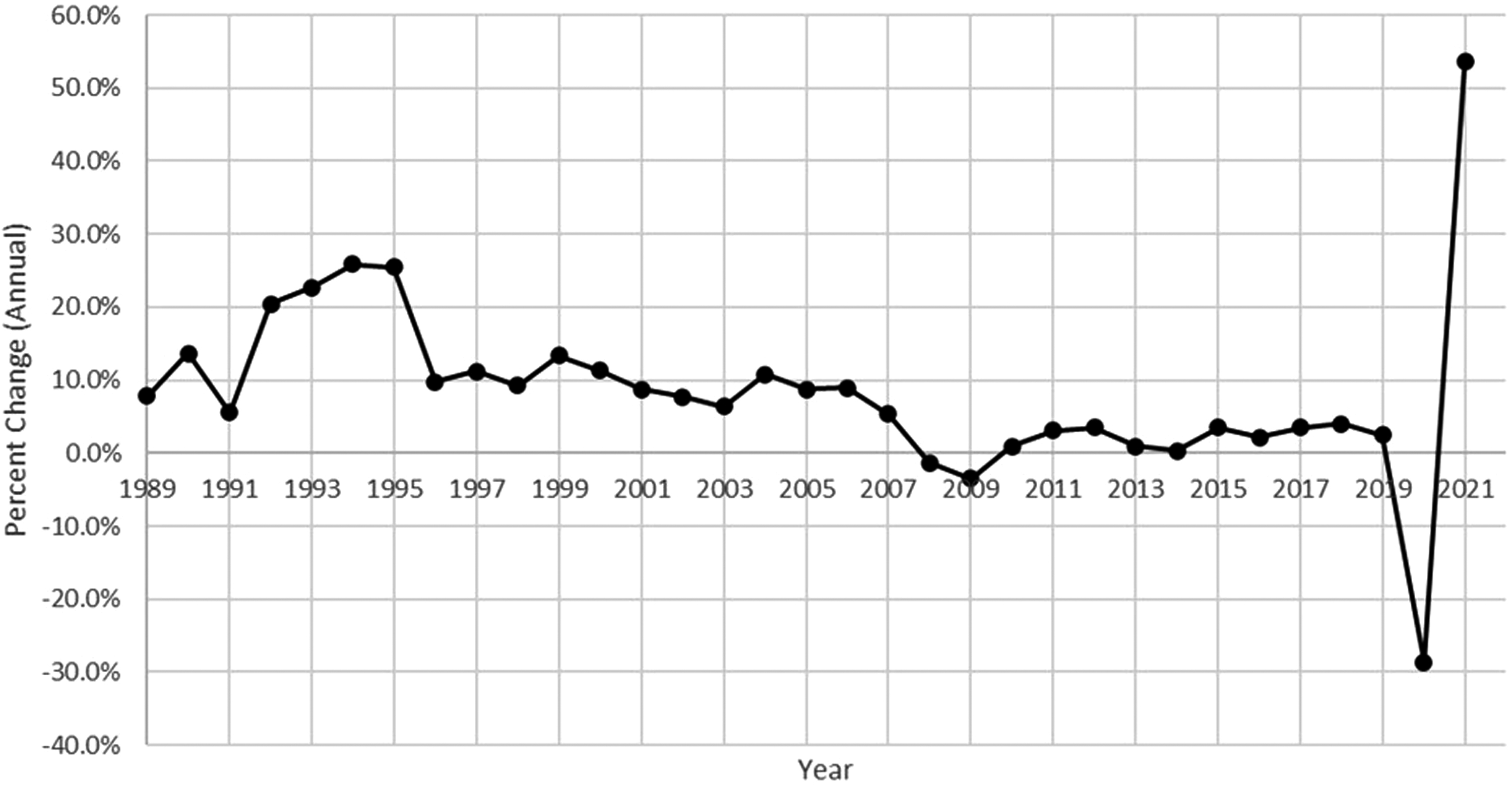
We begin by discussing the two factors that influenced the years of data we employ in our final statistical analysis. The first is data availability. Complete U.S. casino revenue is only available back to 1988, when Indian gaming data started being collected. Second, because we wish to focus on how “normal” business cycle recessions and booms may affect the gaming industry, we exclude from our correlation analysis two time periods we believe are atypical. Fig. 4 shows the annual growth rate of U.S. casino revenue over the entire period of data availability to help illustrate the choices we made on which years of data to exclude.
U.S. Casino Revenue Annual Growth Rates, 1989–2021. Sources: State gaming regulatory agencies; International Gaming & Wagering Business; National Indian Gaming Commission; Casino City's Indian Gaming Industry Report; Meister Economic Consulting estimates
The first period of time we exclude is the recent data influenced by the COVID-19 pandemic. The forced closure of much of the U.S. economy starting in early 2020 created atypical changes in both macroeconomic variables and gaming revenue that are not useful for developing a model that is predictive of future business cycle fluctuations. These changes were both unusual in magnitude (much larger) as well as in timing. By their nature there was no possibility of normal leads or lags, as closures immediately lowered casino revenue as well as affected national macroeconomic variables. Thus, in the correlation analysis, we use data only through 2019 that does include several prior recessions we expect to be more representative of future business cycle related changes.
The second period of data we believe is atypical was the data prior to 1996. Between 1990 and 1996, several midwestern states legalized riverboat casinos, and as a result, revenues in this overall U.S. casino sector grew significantly. Racinos and Indian gaming also grew rapidly. Both of these industry segments experienced annual growth rates exceeding 30% in each year prior to 1996, and even exceeding 100% in at least two of the years (and over 50% in most years). These growth rates were the result of industry expansion rather than business cycle fluctuations. We thus use data for only 1996 forward for our business cycle analysis.
As can be seen in Fig. 4, however, industry growth was still more rapid, on average, between 1996 and 2006 than from 2007 onward. This is caused by the continued rapid expansion in the Indian gaming segment, which experienced an average annual growth rate of approximately 15% between 1996 and 2006, but only 2.6% from 2007 through 2019. However, because the growth rates were fairly constant within each of these two sub-periods (as will be shown more clearly later), we employ statistical methods to correct for this differential growth across these two subperiods of data. Thus, for our analysis of U.S. casino revenue, our final time period of analysis is 1996 through 2019.
B. Identification of macroeconomic variables correlated with gaming revenue
In this section, we provide a correlation analysis that identifies which macroeconomic variables are most closely correlated with U.S. casino revenue using statistically estimated correlation coefficients. As is common practice, to uncover macroeconomic business-cycle-related changes, correlations in the annual growth rates (e.g., annual percentage changes) in all variables are used throughout the analysis. The use of annual growth rates effectively removes any constant long-run trends to focus only on the ups and downs in the data and their correlation with the macroeconomy.
Correlation coefficients (typically denoted as “r” or by the Greek letter “rho,” ρ) are the standard metric used to identify the strength, direction, and timing of the relationships among and between two data series or “variables.” The estimated correlation coefficient between two variables can range from -1.0 to 1.0. A value of 0.0 means the two variables are not correlated (i.e., they are unrelated), a negative value means they are inversely correlated (one rises when the other one falls, and vice versa), and a positive value means they are directly correlated (one rises when the other one rises, and vice versa).
Larger correlation coefficients (i.e., in absolute value, thus those further away from zero and closer to either 1.0 or -1.0) indicate a stronger relationship between the variables. Thus, two variables with a correlation coefficient of 0.45 are more closely and positively correlated than two with a correlation coefficient of 0.19. A correlation coefficient of 1.0 means that two variables are perfectly positively correlated, while a value of -1.0 means that two variables are perfectly negatively correlated.
For most macroeconomic variables, such as measures of household income for example, we would expect a positive correlation with gaming industry revenue because as the economy performs better, consumers are likely to spend more on gaming. For a small number of other macroeconomic variables, such as unemployment, the correlation should be negative because as unemployment increases during recessions, consumers are less likely to have a job and thus be more likely to spend less on gaming.
Which macroeconomic variables may lead ahead of or lag behind casino industry revenue data can also be identified using the estimated correlation coefficients. For each macroeconomic variable, not only do we estimate the correlation coefficient between the variable and gaming revenue data for the same year, but we also examine the correlation coefficients for two prior and two future years.
Because macroeconomic variables are often highly correlated with themselves over time (e.g., unemployment this year is generally correlated with what it was last year), we expect any indicator that is correlated with gaming industry revenue to be correlated for several years in a row. Which year has the largest correlation coefficient identifies which year is most closely related, which is usually but not always the same year. If, instead, a prior (or future) year data has a higher estimated correlation coefficient than same period data, the variable then is concluded to be a significant leading (or lagging) indicator.
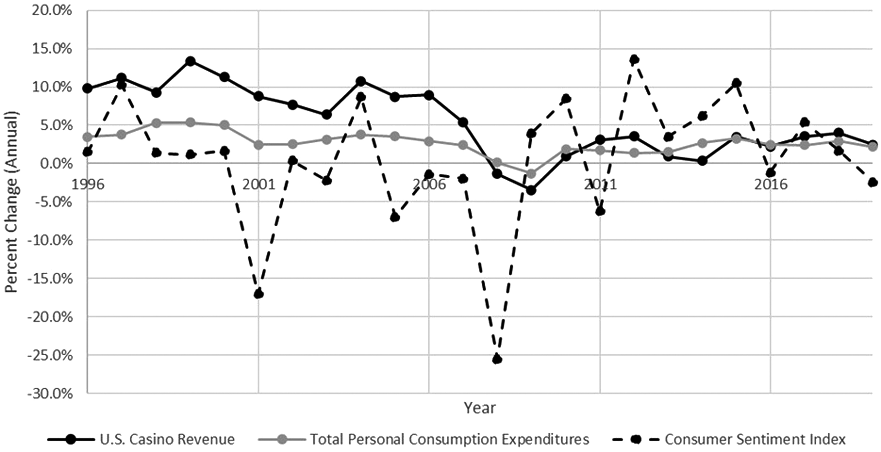
To illustrate the effectiveness of correlation coefficients and what they are measuring, Fig. 5 shows the underlying data for the annual percentage growth rate in U.S. casino revenue along with the annual growth rates of total personal consumption expenditures (PCE) and the consumer sentiment index (CSI) for the 1996 to 2019 period.
U.S. Casino Revenue Correlation with Personal Consumption Expenditures and Consumer Sentiment Index
As can be seen in the figure, the ups and downs of PCE are visually more closely related with the ups and downs of U.S. casino revenue than the CSI. As examples, the large declines in consumer confidence in 2001 and 2011 do not seem to be associated with declines in U.S. casino revenue growth in those (or the following) years. Instead, U.S. casino revenue tracked a similar pattern as PCE.
The estimated correlation coefficient provides a measure of this association and its magnitude. The estimated correlation coefficient between the annual growth rates of U.S. casino revenue and PCE is 0.849, while the estimated correlation coefficient between the annual growth rates of U.S. casino revenue and the CSI is much smaller at only 0.078.
Because the consumer confidence index (CCI) is often thought to be a leading indicator, one might anticipate it is correlated more strongly if one considers the correlation with a one-year time difference. For example, how do changes in the 1997 CSI correlate with 1998 changes in U.S. casino revenue? Indeed, they are more correlated than same year values, but only slightly more. The correlation with a one-year lead in the data is 0.116, higher than the value of 0.078 using data from the same year. It is still much weaker than the correlation with PCE, however. For comparison, the correlation coefficient with PCE is smaller when one considers a one-year lead, 0.772, compared with the previously noted value of 0.849 using the same year data.
The correlation coefficient between two series must surpass a minimum threshold value to be considered “statistically significant” (i.e., statistically different from the value of zero). This threshold depends on the number of years of data one has to analyze. For the data shown in Fig. 5, the threshold value is 0.4044. 31 Thus, only in cases where the correlation exceeds roughly 0.40 (or is negatively larger than -0.40), is it generally accepted as a sound basis for statistical research or forecasting.
Thus, U.S. casino revenue is indeed significantly correlated with PCE as the correlations far exceed this threshold value. In contrast, one would conclude that the correlation with the CSI is not strong enough to be considered statistically significant—it is indistinguishable from a correlation coefficient value of zero in the time period of analysis. Thus, PCE could make a good candidate for a forecasting model of U.S. casino revenue, while the CSI is not statistically reliable enough to use for prediction purposes.
Correlations with U. S. casino revenue
We estimated correlation coefficients for the annual growth rates of U.S. casino revenue with all of the macroeconomic variables we collected and considered. Table 3 below shows these correlation coefficients. Correlations that rose to the level of statistical significance are noted with an asterisk in the table. For each macroeconomic variable that has a statistically significant correlation, the year with the highest correlation is shown in italics.
Correlation Coefficients for U.S. Casino Revenue and Macroeconomic Variables (Annual Growth Rates, 1996–2019)
Notes: * indicates statistical significance (5% level, two-tailed test).
Source: Meister Economic Consulting analysis.
As can been seen in the table, when examining annual growth rates, several of the macroeconomic variables have significant correlations with total casino revenue: Personal Consumption Expenditures, Disposable Personal Income, Average Household Income, Gross Domestic Product, Male Population, and Population Aged 20 to 64.
It is important to note that these correlations are pair-wise correlations between each variable and U.S. casino revenue, and do not control for the other variables. We do so just to identify which variables to consider for our analysis and to look for possible leading and lagging indicators. Our forecast model will employ a more sophisticated statistical analysis to be able to examine these relationships controlling for multiple variables at once. For example, over time PCE grow as population grows, and U.S. casino revenue grows as well. Thus, both PCE and population are positively correlated with U.S. casino revenue. But as our forecasting models show later in this article, it is really the consumption spending aspect that is the driver of U.S. casino revenue, and once the contribution of the growth of consumption spending is accounted for, measures of population growth have no independent effect over and above how the population growth is increasing consumer spending.
As shown in Table 3, the most highly correlated variable with U.S. casino revenue is PCE, with a correlation of 0.849. This is why it was chosen for the graphical correlation example presented earlier. The second most highly correlated macroeconomic variable is GDP, with a correlation coefficient of 0.793. These are the two top candidates to employ as the basis for a forecasting model, and their highest correlations are shown in bold italics. While disposable personal income and average household income do have significant correlations, they are much smaller correlations than for PCE or GDP, and thus would provide a significantly less accurate basis for forecasting of U.S. casino revenue.
We thus develop our main models using PCE and GDP. The correlations for the two population variables (male population and population aged 20 to 64), while smaller than for the main macroeconomic indicators of PCE and GDP, are actually most correlated at their two-year lag. This would oddly imply that changes in today's population trend could be used to predict U.S. casino revenue trends two years into the past, which is the opposite direction of effect we were looking for as the basis for a forecasting model. This may likely be an artifact of the underlying data as the U.S. Census Bureau only does a true census every 10 years, and simply estimates population trends between those years for the data they publish. However, as was mentioned before, once our forecasting models control for measures of economic activity, these population variables are no longer significant explanatory variables.
Also, it is worth explicitly noting the macroeconomic variables in the table that are not significantly correlated enough with U.S. casino revenue to be reliable enough for forecasting: Unemployment Rate, S&P 500 Composite Price Index Average, Consumer Sentiment Index, Housing Starts, Federal Funds Rate, Personal Savings, and Personal Savings Rate.
With the exception of the population variables, for all other macroeconomic variables that have a statistically significant correlation, the year with the highest correlation is the same year data, implying that none of the series are truly leading or lagging indicators of the industry. Instead, the industry moves closely in timing with these macroeconomic variables.
To ensure our results were robust, we also performed a similar correlation analysis with subsamples of U.S. casino revenue: (a) the casino industry broken down by individual segments (i.e., commercial casinos, racinos, and Indian gaming); and (b) several individual casino markets in Nevada and Missouri. We also performed the analysis using gross product for the entire NAICS Industry 7132 (gambling industries). In all cases, the annual growth rates of PCE and GDP were the two macroeconomic variables most closely correlated with the annual growth rates for U.S. casino revenue, and in some cases GDP had the highest correlation. We are thus very confident these are the two best macroeconomic variables we tested on which to forecast casino revenue data.
To further explore the possibility of leads or lags, we also considered quarterly data for a single market of casinos within Missouri, for which we had complete data readily available. We wanted to determine if the use of annual data above in our main analysis was perhaps providing too long of a lead/lag to pick up any significant results. Our results still showed the same two variables as most strongly correlated, with the highest correlations at a two-quarter lead for PCE and a three-quarter lead for GDP.
These could point to some ability to use data if it can be obtained quarterly or more often, but it also simply could be the result of the Missouri economy itself being slightly behind the national economy, which is likely for a state in the mid-west whose largest industries are related to farming and agriculture. However, the government agencies that release quarterly data on the economy take time to compile and release it publicly once a quarter or month is complete. Thus, at any given time the actual data available may be up to a few quarters or months behind the current period anyway, limiting the usefulness of this finding. Importantly, two or three quarters or months is still within the single year framework we identified earlier suggesting our finding that same year annual data is the best to develop our forecasting model.
We now turn to developing U.S. casino revenue forecasting models based upon the macroeconomic variables with which we found significant correlations.
C. Forecast of casino revenue using macroeconomic variables
The previous section identified the annual growth rates of PCE and GDP as the macroeconomic variables most valuable for forecasting the annual growth rate of U.S. casino revenue over the business cycle. In this section, we estimate the actual forecast models based upon these variables using regression analysis.
Regression analysis is a statistical method used to estimate the strength and nature of the relationship between one main variable of interest (the “dependent variable,” here U.S. casino revenue), and one or more other variables on which it may depend (the “independent variables” or “explanatory variables,” here our macroeconomic variables). In doing so, it can estimate the linear relationship between the dependent variable and any one or more of the independent variables, while controlling for other variables that may also have influence. Regression analysis is used extensively in economic research to uncover the causal relationships between variables and to develop models for forecasting purposes.
In general, the regression analysis forecast model specifies the relationship as:
The dependent variable in the model, U.S. casino revenue growth, is a function of one or more independent variables reflecting macroeconomic growth as measured by various metrics (e.g., PCE and GDP). The two parameters of particular interest in the model to be estimated with historical data are the constant (α) and the coefficient(s) on the macroeconomic variable(s), denoted by (β). The variable ɛ t is the random error in the data (i.e., the estimated differences between the forecasts and actual data) and is not pertinent to interpreting the parameters of interest.
The coefficient for a macroeconomic variable (β), which is a slope coefficient, may actually be interpreted similar to a stock's “beta.” Thus, as a hypothetical example, an estimated (β) coefficient of 1.25 on a macroeconomic growth variable would imply U.S. casino revenue fluctuates over the business cycle by about one and a quarter (1.25) times as much as the underlying macroeconomic variable (thus, a 1.0% more or less rapid growth in GDP, for example, would be associated with a 1.25% more or less rapid growth in U.S. casino revenue).
The ability of each forecasting model to fit the data is measured by the R2 for each estimated model, which ranges from 0, when it is a poor fit, to 1.0, when it is a perfect fit. It can roughly be interpreted as the percentage of the variation in the data explained by the model, so an R2 of 0.78 means the model explains 78% of the variation in the underlying data. The model provides better quality forecasts as R2 increases.
It is also typical to provide a second measure to determine the overall fit of the model, the adjusted R2, which is based on the standard R2 but adjusts for the number of variables used in the model. The adjusted R2 is generally considered to be the superior measure because the normal R2 increases each time a variable is added to a model, even if the variable does not meaningfully improve the model beyond the variables already included. The adjusted R2 does not increase when adding a variable to a model unless it contributes to explaining the variable of interest (and is thus generally lower than the normal R2). When comparing various models, we can determine the one that is superior by the higher adjusted R2.
Table 4 shows the results of our forecasting models for the annual growth rate of U.S. casino revenue using the two most correlated macroeconomic variables, the annual growth rates of PCE and GDP. We estimate both models with and without including the additional population variables that were significantly correlated when considered alone with U.S. casino revenue. We also include a variable that accounts for the significantly higher average growth rates prior to 2007 as compared to 2007 onward, as previously discussed in section VI-A. This type of variable is commonly referred to as a dummy variable.
Results of Regression Models to Forecast U.S. Casino Revenue Growth, 1996–2019
Notes: P-values reported in parentheses. * indicates statistical significance at 10% level. ** indicates statistical significance at 5% level. *** indicates statistical significance at 1% level.
Source: Meister Economic Consulting analysis.
In our models, a value of 1 is used for all years prior to 2007, and a value of 0 for all years from 2007 forward. In this way, the dummy variable can account for a general difference in U.S. casino revenue before 2007 as compared to 2007 and later, leaving the relationship between U.S. casino revenue and the macroeconomic variable in each model to be more accurately reflected without other confounding factors.
For all models, the macroeconomic variables are statistically significant in terms of helping predict casino revenue (all at the 1% significance level, which is very strong). Our dummy variable that removes the pre-2007 trend growth difference is also significant at the 1% level, and the coefficient estimates suggest that revenue growth was on average around 4.7 to 5.5% more rapid in the earlier years relative to the later years.
When the population variables (male and age 20 to 64) are included, they are not statistically significant. This implies that once we account for the trends in PCE or GDP, the population variables do not add additional relevant information to the predictive power of the model. This is also confirmed by the adjusted R2, which is higher in both cases for the models excluding these population variables. We thus continue our analysis discussing and using the best two models, shown by Models 1A and 2A in Table 4.
The models provide an excellent fit of the data according to the adjusted R2 values, explaining nearly 90% of the variation in U.S. casino revenue growth. These are very strong results. The difference in the fit (adjusted R2) of the models using PCE and GDP is only 0.0023 percentage points, essentially meaning they provide virtually equally good forecasts of the U.S. casino revenue data.
The quality of fit of the models is best assessed visually in Fig. 6 showing the actual data versus the forecasts from the two models. Both models do a good job of capturing the declines in the U.S. casino revenue during the economic recessions in 2001 and 2007–2009. They also capture well the upturns in revenue associated with the economic recoveries and economic boom periods after those recessions, although both models predict casino revenue recovering a little sooner/faster than it actually did after the 2001 recession.
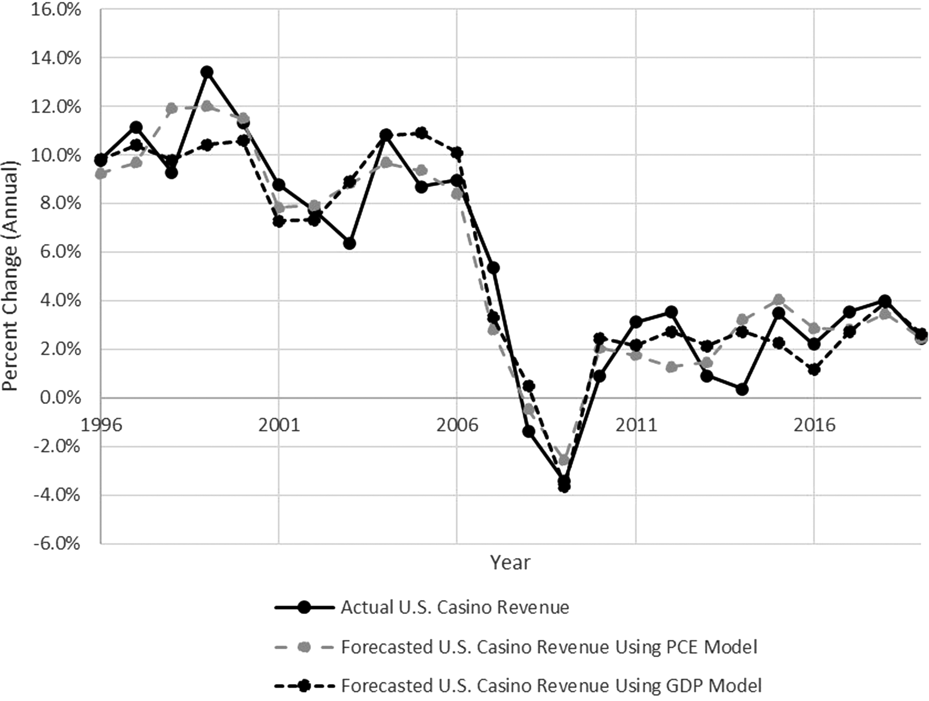
Actual Versus Forecasted U.S. Casino Revenue, Personal Consumption Expenditures and Gross Domestic Product Regression Models, 1996–2019. Sources: U.S. Bureau of Economic Analysis; Moody's Analytics; Meister Economic Consulting
Based upon our earlier correlation analysis, we also checked to see if the data from one year earlier for PCE or GDP (and the other variables with significant correlations) would make a valuable forecasting model. These models were significantly worse, always missing the onset of recessions by one or more years, while the same year data from our PCE or GDP models did not. This led us to the unambiguous conclusion that there were simply no macroeconomic variables that were reliable enough to be used as a basis for a one year into the future forecast of U.S. casino revenue. Instead, relying upon good forecasts of future year data on GDP or PCE in our models to forecast future U.S. casino revenue is the better approach to obtain reliable forecast estimates.
Before moving on to our future U.S. casino revenue forecasts, another interpretation of our models worth briefly discussing is the estimated cyclical stability of U.S. casino revenue implied by our estimated coefficients (β) that can be interpreted similar to the beta for a stock.
Using the models for the truncated time period of 1996 through 2019, the estimated coefficients (β) suggest that for every 1 percentage point the growth rate of PCE increases (or decreases), the growth rate of U.S. casino revenue changes in the same direction by slightly more than 1.43% (the coefficient for PCE is 1.4346 in Model 1A in Table 4). For GDP, each 1 percentage point increase (or decrease) in the growth rate of GDP causes casino revenue growth to change in the same direction by approximately 1.03% (the coefficient for GDP is 1.0332 in Model 2A in Table 4). The interpretation of these numbers suggests that casino revenue fluctuates slightly more (about 1.43 times as much) than PCE, but about equally as much (only 1.03 times as much) as the overall economy as measured by GDP.
D. Forecasts of future U.S. casino revenue growth
Given the public availability of data forecasts, the GDP model is probably our most useful and reliable for the purposes of forecasting future U.S. casino revenue growth rates. Using the results of that model (Model 2A in Table 4), we have the following equation into which we can plug a forecast for GDP growth to obtain a U.S. casino revenue growth forecast:

For comparison purposes, we also consider the PCE model. Using the results of that model (Model 1A in Table 4), we have the following equation into which we can plug a forecast for PCE growth to obtain a U.S. casino revenue growth forecast:
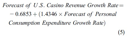
As an example, Moody's Analytics, a reputable provider of research, data, and analysis, had forecast the growth rate of GDP to be 5.2435% for 2023. The forecasted growth rate of U.S. casino revenue based upon this from the GDP model above would be calculated as: −1.6104 +(1.0332×5.2435)=3.81%.
Moody's Analytics provides future estimates of both GDP and PCE. For GDP there are also a couple of other readily available sources of future estimates, including the Federal Reserve Bank of Philadelphia's Livingston Survey and the Survey of Professional Forecasters. 32 However, these data sources do not offer forecasts as far into the future as Moody's Analytics. The most recent Livingston Survey (June 2023) and Survey of Professional Forecasters (May 2023, Second Quarter) both have forecasts for only 2023 and 2024.
Table 5 shows the forecasts of the annual growth rate for U.S. casino revenue based on our models and these variety of forecasts of future macroeconomic data for the next five years, 2023 through 2027. In terms of the various forecasts for 2023 using GDP, the three sources provide similar results. Moody's Analytics forecast for the final annual growth of GDP in 2023 (5.75%) is slightly higher than the growth rates forecast from the Survey of Professional Forecasters (5.40%) and the Livingston Survey (5.29%). Because Moody's forecast for GDP growth is higher, this leads to a slightly higher forecast for U.S. casino revenue growth in 2023 of 4.33% based on the Moody's GDP forecast, and slightly lower but similar forecasts of 3.86% based on the Livingston Survey GDP forecast, and 3.97% based on the Survey of Professional Forecasters GDP forecast as of July 2023.
Forecasts of U.S. Casino Revenue Annual Growth Rates, 2023–2027 Based on Gross Domestic Product and Personal Consumption Expenditure Models
Source: Meister Economic Consulting analysis.
Looking further into the future, for 2024, there is a larger difference among the sources for their forecasts of GDP growth, which results in more variance in the predictions for the growth of U.S. casino revenue. The forecasts of GDP growth in 2024 are 3.64% from Moody's Analytics, 3.70% from the Survey of Professional Forecasters, and 2.99% from the Livingston Survey. This leads to a wider range in the forecasts of U.S. casino revenue growth for 2024 of 2.15%, 1.48%, and 2.21%, respectively. Notably, all three sources predict a slowdown of GDP growth in 2024 relative to 2023, and thus the forecasted growth of U.S. casino revenue is also quite a bit lower in 2024 for all three sources than it is for 2023.
For 2024 through 2027, there are not large differences between the forecasts from the models using Moody's Analytics GDP forecasts versus Moody's Analytics PCE forecasts. The larger difference for 2023 is due to Moody's forecasting 5.75% for GDP growth while only 1.56% for PCE growth. This leads to a large differential in the forecasted growth rate for U.S. casino revenue in 2023 from the two models using Moody's forecast data. As previously noted, the forecasted growth rate for U.S. casino revenue in 2023 is 4.33% using Moody's Analytics GDP forecast, but it is only 2.32% using their forecast of PCE. The difference in the U.S. casino revenue forecasts based on Moody's Analytics data for GDP and PCE come more into alignment in 2024 and beyond, with the differential falling to as low as 0.35% in 2027 (3.05% versus 2.70%). 33
VII. CONCLUSION
In this article we have attempted to provide an overview of how the U.S. economy, and the business cycle of recessions and booms it undergoes, influence the U.S. casino sector. We analyzed a variety of macroeconomic indicators and their relationships with the U.S. casino sector.
We tested the strength of correlations with 13 major macroeconomic indicators including, among others, measures of the stock market, interest rates, population, housing, unemployment, personal income, and GDP. We find that the most highly correlated variable with U.S. casino revenue is PCE, with a correlation of 0.849. The second most highly correlated macroeconomic variable is GDP, with a correlation coefficient just slightly smaller at 0.793. Both are most highly correlated in the same period of data, rather than with a lead or lag in the relationship.
Based on these correlations, we then used these two macroeconomic indicators (PCE and GDP) as the basis for developing statistical forecasting models of U.S. casino revenue growth. The models provide an excellent fit of the data, explaining nearly 90% of the variation in U.S. casino revenue growth. The difference in the fit of the models using PCE and GDP is only 0.0023 percentage points, essentially meaning they provide equally good forecasts of U.S. casino revenue.
Similar to the way one would interpret a beta for a stock, our models suggest that for every 1 percentage point the growth rate of PCE increases (or decreases), the growth rate of U.S. casino revenue changes in the same direction by slightly more than 1.43%. For GDP, each 1 percentage point increase (or decrease) in the growth rate of GDP causes U.S. casino revenue growth to change in the same direction by approximately 1.03%. The interpretation of these numbers suggests that casino revenue fluctuates slightly more (about 1.43 times as much) than the average of all consumer spending, but about equally as much (only 1.03 times as much) as the overall economy as measured by GPD. These numbers are interesting to interpret in light of the old claim that the casino sector is “recession proof,” as while it is true that casino revenue growth fluctuates only 3% more than GDP growth, once the measure of economic activity is narrowed to consumption expenditures only, the stability of casino revenue over the business cycle is much lower. Fluctuations in the growth of consumer expenditures are associated with a 43% greater fluctuation in casino revenues.
Based on three reliable sources of economic forecasts for U.S. GDP growth and PCE (Moody's Analytics, and Livingston Survey and Survey of Professional Forecasters from the Federal Reserve Bank of Philadelphia) we provide forecasts of U.S. casino revenue growth through 2027. Our forecasts generally show U.S. casino revenue growth slowing significantly in 2024.