Predicting Influenza A Tropism with End-to-End Learning of Deep Networks

Abstract

The type of host that a virus can infect, referred to as host specificity or tropism, influences infectivity and thus is important for disease diagnosis, epidemic response, and prevention. Advances in DNA sequencing technology have enabled rapid metagenomic analyses of viruses, but the prediction of virus phenotype from genome sequences is an active area of research. As such, automatic prediction of host tropism from analysis of genomic information is of considerable utility. Previous research has applied machine learning methods to accomplish this task, although deep learning (particularly deep convolutional neural network, CNN) techniques have not yet been applied. These techniques have the ability to learn how to recognize critical hierarchical structures within the genome in a data-driven manner. We designed deep CNN models to identify host tropism for human and avian influenza A viruses based on protein sequences and performed a detailed analysis of the results. Our findings show that deep CNN techniques work as well as existing approaches (with 99% mean accuracy on the binary prediction task) while performing end-to-end learning of the prediction model (without the need to specify handcrafted features). The findings also show that these models, combined with standard principal component analysis, can be used to quantify and visualize viral strain similarity.

Deep learning techniques have the ability to learn how to recognize critical hierarchical structures within the genome in a data-driven manner. The authors designed deep convolutional neural network models to identify host tropism for human and avian influenza A viruses based on protein sequences and performed a detailed analysis of the results. Findings show that deep convolutional neural network techniques work as well as existing approaches while performing end-to-end learning of the prediction model (without the need to specify handcrafted features).

Rapid virus classification is important for the diagnosis of infections and in the response to natural outbreaks or intentional release.^1-3 Comparisons of sequences can provide biological insights into viral traits such as host specificity or transmissibility. Understanding host specificity and transmissibility is particularly relevant to influenza viruses, which are able to infect multiple hosts and regularly emerge as significant drivers of seasonal disease patterns, with the potential to cause a pandemic.⁴ While influenza strains infect a wide range of vertebrates, zoonotic transmissions rise with increased animal proximity and contact with humans.^5,6

A major source of zoonotic transmissions derives from avian strains that infect domesticated birds.⁷ Swine are susceptible to infection by swine, human, and avian influenza strains; coinfections can sometimes result in novel reassortment of proteins from different viral strains. Alternatively, virus adaptation to new hosts can evolve from alterations to the primary and possibly secondary structure of viral proteins, particularly the host receptor protein hemagglutinin (HA) and neuraminidase (NA). The severity of infections of zoonotic influenza virus—that is, those that hop from one host to another—ranges from negligible to fatal. Thus, monitoring of influenza virus adaptation is of critical importance for understanding, preventing, and mitigating disease outbreaks.

Influenza tropism, like nearly all phenotypes, is dictated by the viral proteome. One approach for determining tropism takes in large amounts of basic input information (protein sequences) and assigns the strain to one of several categories. Eng et al¹ constructed machine learning random forest classifiers to achieve high-accuracy classification of influenza A tropism, based on input features that characterize amino acid frequency and composition as well as biochemical properties of amino acids, such as transition and distribution features for the hydrophobicity, normalized van der Waals volume, polarity, polarizability, charge, and solvent accessibility. One of the keys to this approach is the use of hand-coded features that are known a priori to be helpful for viral property characterizations.

Recently, deep learning methods (particularly CNNs) have been very successful in a number of machine learning problems,^8-10 although to our knowledge they have never been applied to the viral tropism prediction problem. Deep CNNs offer a number of advantages over more traditional machine learning methods, such as the ability to automatically learn features that support classification, instead of relying on hand-coded features. These features are advantageous over handcrafted ones in that they can learn features a human might not know of as important. In addition, many of the features learned by deep networks can be reused in other tasks. Therefore, we might expect that low-level features extracted from the viral proteome to support host tropism predictions could also be leveraged in other viral phenotype prediction tasks.

The main objectives of the research presented in this article are (1) to design variations of deep network architectures that facilitate accurate end-to-end learning of tropism prediction models, (2) to produce insights about the link between the influenza A proteome and host tropism by examination of the trained models, and (3) to use reduced-dimension visualizations to draw conclusions about the evolution of historical viral samples.

Methods

Data and Data Preparation

All viral sequences used in these experiments were downloaded from GenBank.¹¹ The BioTools GenBankParser¹² was used to parse the GenBank viral sequences into FASTA files. The GenBankParser encodes sequence metadata in the FASTA header in a structured format. Influenza A sequences were selected using the metadata for organism name. The Dawn program was used to align the influenza A protein sequences.¹³ We used version 1.0, with the input file being the FASTA protein sequences. Due to the high diversity in the neuraminidase sequences, the Clustal Omega program was used to align them.¹⁴ We used version 1.2.4, with the parameters being the input and output file. The experiments used information from 7 different viral proteins: HA, M, M1, NEP, PA, PB, and PB1-F2. Some experiments also used NA. A grand total of 306,659 strains were analyzed.

The influenza strain names were used to classify viruses as human or avian. Viral sequences with no strain information were excluded. For each type of protein, a histogram of number of missing elements per strain showed clear inflection points where the majority of strains had less than a certain number of missing elements. The exact threshold was calculated separately for each protein. Shorter partial length sequences were removed. For each protein, unless otherwise stated, 66% of the data was randomly chosen for training, and the remaining 33% was reserved for testing. The number of resulting data samples is displayed in Table 1.

Table 1.

Database Summary

Protein	Initial No. Sequences	No. Usable Sequences	No. Human Sequences	No. Avian Sequences
HA	87,571	60,109	23,891	36,218
M	54,587	44,159	17,232	26,927
M1	53,371	43,306	16,566	26,740
NEP	4,090	3,714	1,889	1,825
PA	64,082	35,388	15,665	19,723
PB	42,904	34,818	15,461	19,357
PB1-F2	54	47	18	29

To convert the data to a usable format, each aligned protein sequence was converted into a LxA matrix where L is the length of the aligned sequence (in this case, several hundred amino acids) and A is the number of unique amino acids (in this case, 26). Amino acid sequences that were shorter than L were zero-padded to this length. The amino acid at each space was represented by one-hot encoding—that is, if the nth amino acid was present at point i, then the nth element at point i would be 1, and all other points at i would be zero. For all classification methods, each viral protein had a separate classifier.

The Jmol program¹⁵ was used to visualize deep CNN results on the Protein Data Bank (PDB) structures 4GXX¹⁶ for hemagglutinin and 2HTY¹⁷ for neuraminidase.

Classification Methods Investigated

A number of statistical, deep learning, and conventional machine learning algorithms were applied to tropism prediction based on the 7 encoded influenza aligned protein sequences (HA, M, M1, NEP, PA, PB, and PB1-F2). The algorithms are described briefly below.

Prediction Based on Priors

This method measures the percentage of training data that was of each class and simply predicts all strains belong to the highest frequency species tropism. For example, if 60% of the training data is avian, the classifier predicts avian for all test samples. This approach establishes a trivial performance baseline based on prevalence of sample types.

Prediction Based on Strain Designation

This method is similar to the method described above, but instead of prediction based on the relative abundance of each class in the whole dataset, the classifier predicts based on the relative abundance of each class within the corresponding strain designation (eg, H1N1). This experiment used designations based on hemagglutinin (H) and neuraminidase (N). This is somewhat indicative of host tropism, because certain designations (or strains altogether) are highly correlated with certain hosts. For example, in H1N1 sequences, the vast majority of strains are human. If this approach guesses “human” for every H1N1 virus seen in the dataset, the guessed label will almost always be correct. This is, in essence, a more nuanced version of the prediction based on priors.

K Nearest Neighbors

This method uses edit distance (Levenshtein distance) between strains as a distance metric and predicts the class label via the K nearest neighbors in the training set.¹⁸ From values 1 to 10, K = 5 produced the results with the highest accuracy.

Random Forest

This is largely a replication of the techniques used by Eng et al.² As described earlier, this approach feeds selected biochemical properties of amino acids into a random forest classifier, which generates multiple (in our case, 10) decision trees on random subsamples of the data and chooses the majority prediction across all trees for each new data point.

Baseline Convolutional Network

A convolutional neural network is a deep learning method characterized by a series of convolutional functions. A CNN takes an input tensor (which, in this context, is a multidimensional vector) and runs numerous convolutions over it in order to transform the data into an output image. The output of each layer is a NxF matrix, where N is the output length (which may be less due to layer processing) and F is the number of features. “Features” in this case refers to a series of channels that can take on a range of numbers denoting characteristics of the particular point. For example, an RGB image has 3 features, in this case representing the red, green, and blue values of the pixels. In a CNN, each feature dimension is calculated from the same convolutional filter in the layer (ie, the same processing function), although the result might not have a human-interpretable explanation. At the end of each layer is a rectified linear activation (relu) unit, which sets all negative values to zero. This provides nonlinearity, which allows the neural network to fit arbitrary, nonlinear functions.

Each layer in a convolution can be one of several functions. Convolutional and relu units were described previously. There are also batch-normalization (batchnorm) layers, which normalize the data currently passing through the network to stabilize the network output, and maxpool layers, which take neighborhood of adjacent values in an input and return the largest value. In our case, some convolutional and maxpool layers have a stride of N, which means that the layer skips N spots after performing a function on a neighborhood. This reduces the dimensions of the output. The CNN is considered an “end-to-end” model because it can take data, extract features, and classify data all in one step. This is in contrast to traditional methods, such as random forest, that require 2 separate steps for feature extraction and classification. “End-to-end” is generally preferable because it automates more of the classification process.

The baseline CNN is modeled on the architecture referred to as DeepBind.³ It uses only one convolutional layer as originally proposed, and so the network is not truly “deep” in the classic sense of deep neural networks. The convolution is implemented as a 1-dimensional, multichannel convolution along the length of the sequence. There is 1 input channel for each input amino acid, as well as several for special symbols representing alignment gaps and unknown amino acids (“–” representing a gap, and “X” representing a wildcard or unknown amino acid). The model applies a length-3 convolution window, since this is the minimum window size needed to capture low-level sequential patterns, and it has been used frequently in other convolutional networks.^10,19 The model training process used standard back-propagation on the training sequences, with a batch size of 1,024. Half of the data were used for training, 25% for validation (determining the optimal number of iterations), and 25% were reserved for test data. A maximum of 1,000 iterations of back-propagation were found to be sufficient for model convergence. A visualization of the full architecture is shown in Figure 1. Note that this network performs similar feature extraction to a genome-wide analysis in that the system associates genetic loci with phenotypic traits.

Figure 1.

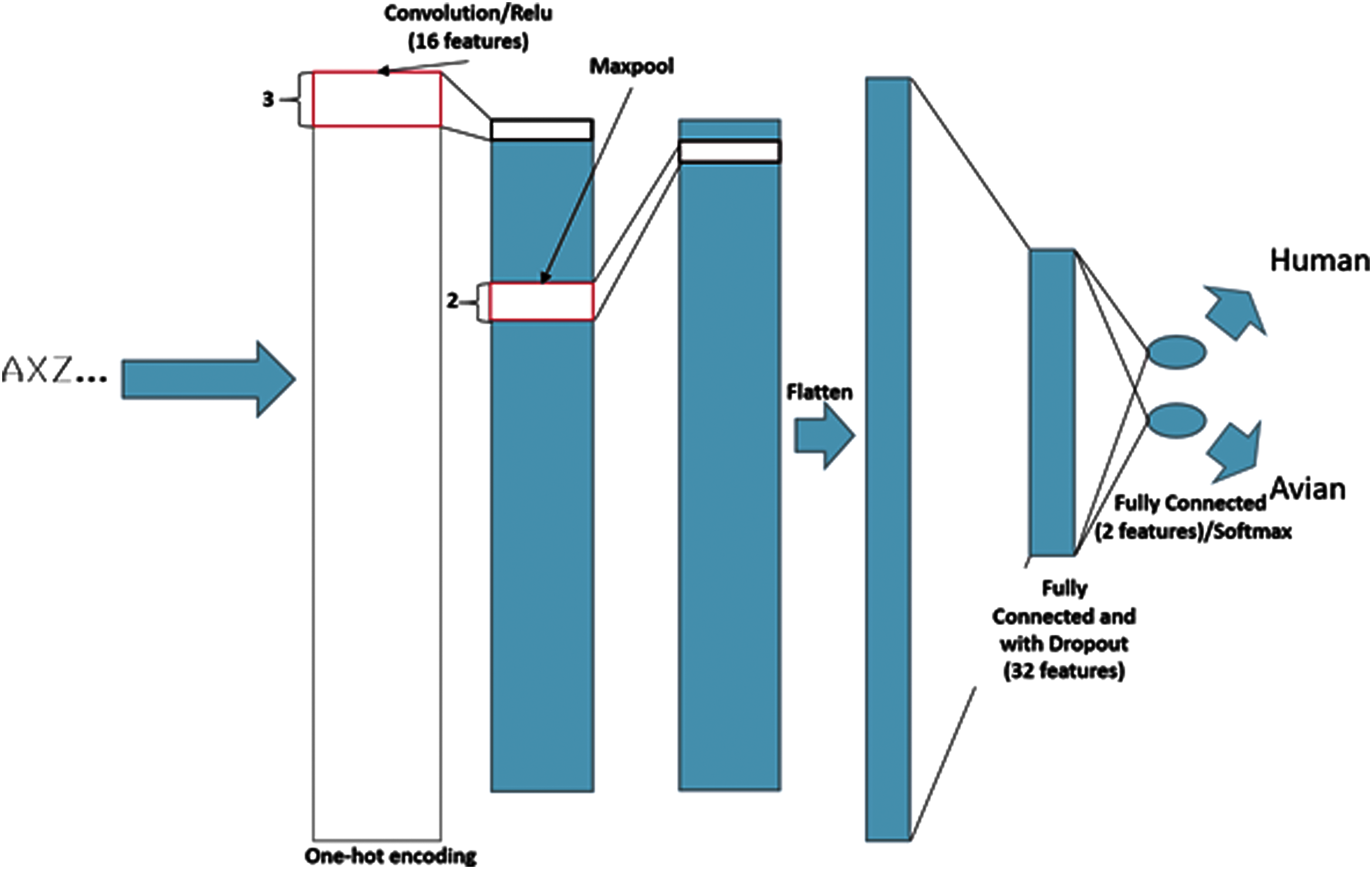
A visualization of the baseline CNN. Unless otherwise indicated, all maxpool and convolution layers have a stride of 1. Color images are available online.

This network trained very quickly, taking only a few minutes to finish. It is important to contrast the features used in both CNNs and random forests. The random forests in work referenced use global features, made by performing specific operations on the entire sequence that are believed to be important to tropism. The CNN, however, essentially learns a mapping from specific amino acids in specific locations to tropism, with each additional layer becoming a mapping of responses over more and more layers. Thus, the CNN is able to estimate tropism by learning specific location combinations of amino acids. Similarly, many of the tropic properties of the molecules (particularly what cell proteins the molecule can bind to) are determined by the specific sequence of amino acids. Thus, the CNN captures the features of the molecule necessary to determine its tropism.

Tailored CNN

The large neural network was built with a similar notion in mind. In this case, “tailored” means that the network was specifically built for this problem. This is contrasted with the baseline CNN, whose architecture is very basic and often used as a baseline in machine learning research. In this case, our network was determined with inhouse software that automatically selects an optimal architecture for a given dataset. The model training process used standard back-propagation on the training sequences, with a batch size of 128. Half of the data were used for training, 25% for validation (determining the best architecture), and 25% were reserved for test data. The architecture was trained until convergence (measured with the validation data).

The tailored CNN is a natural extension of the baseline CNN, but it includes additional layers and features to improve its ability to characterize hierarchical structures within the sequence data. It also used batch-normalization layers after every maxpool layer to aid in training.²⁰ Improving the architecture required experimentation. The results of these trials confirmed that deeper networks (with multiple convolutional layers) consistently improve performance. In some cases, increasing the number of feature channels in each layer does as well, allowing for more variation in pattern expression captured by the model. This network was larger than the previous network, but nonetheless trained relatively quickly. The network finished training in under 1 hour in all experiments. The specifics of this architecture are depicted in Figure 2.

Figure 2.

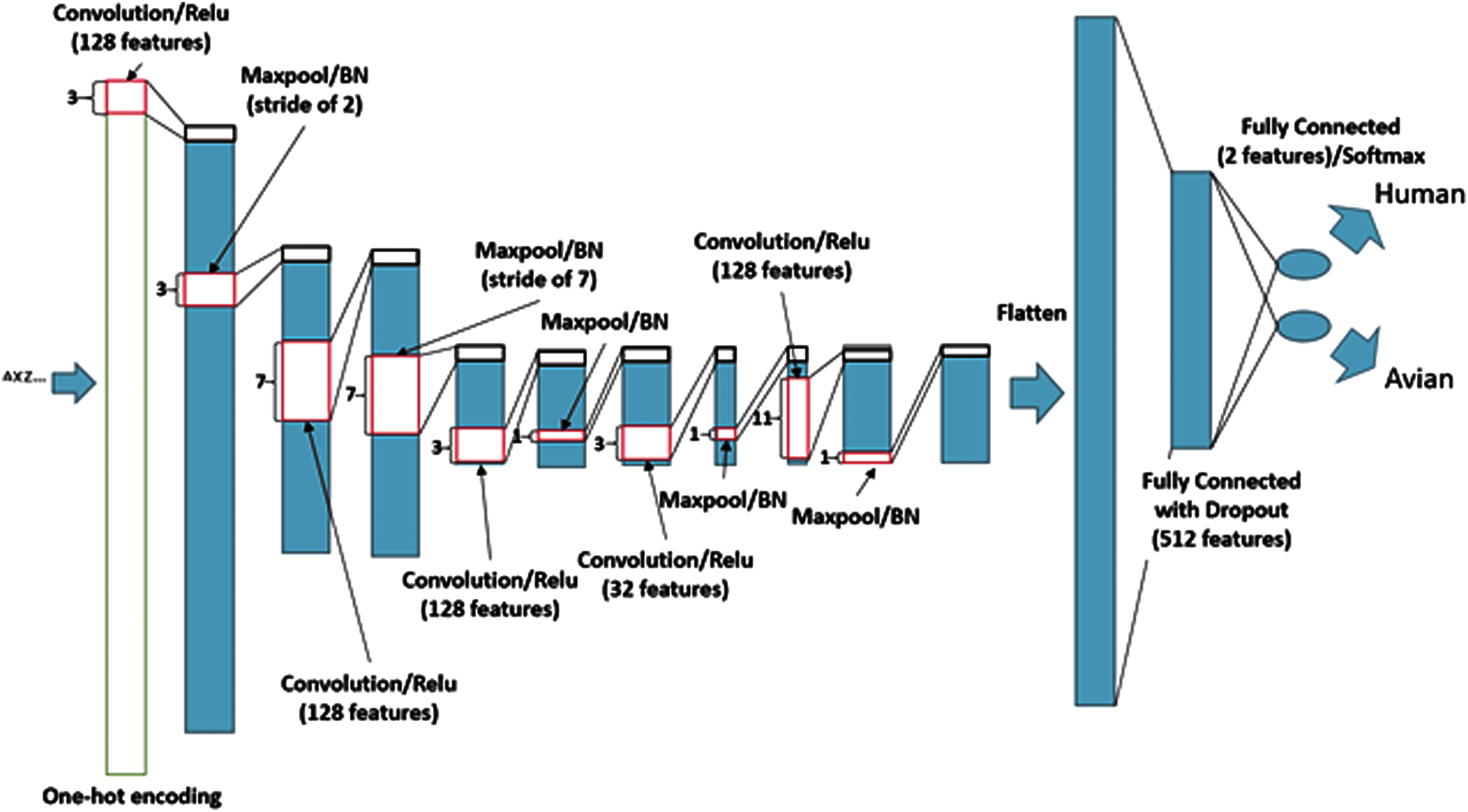
A visualization of the tailored CNN. Unless otherwise indicated, all maxpool and convolution layers have a stride of 1. Note. BN = batch normalization. Color images are available online.

Results

Classification Results

Table 2 lists the accuracy of the classifiers enumerated previously. Although the random forest method outperforms the baseline CNN, the results are very close, given the significant work needed for feature selection on the random forest that the CNN did not need. This shows clearly that CNNs are well suited to this problem—even a small network produces compelling results. Furthering this claim, the tailored CNN has the best performance, performing as well as all other methods.

Table 2.

Accuracy of Tropism Classification (accuracy is percent total correctly guessed strains)

	Accuracy
Protein	Random Prediction	Prediction Based on Priors	Prediction Based on Strain (H+N)	Edit Distance + KNN (k = 5)	Random Forest	Baseline CNN	Tailored CNN	95% Conf. Interval for Tailored CNN
Mean	0.5	0.58	0.948	0.979	0.990	0.971	0.990	n/a
HA	0.5	0.60	0.965	0.991	0.991	0.990	0.992	(0.991,0.993)
M	0.5	0.60	0.961	0.985	0.986	0.985	0.986	(0.985,0.987)
M1	0.5	0.63	0.963	0.985	0.987	0.982	0.987	(0.986,0.988)
NEP	0.5	0.51	0.955	0.981	0.987	0.983	0.989	(0.985,0.922)
PA	0.5	0.58	0.957	0.986	0.986	0.968	0.986	(0.985,0.987)
PB	0.5	0.56	0.956	0.990	0.990	0.974	0.994	(0.993,0.995)
PB1-F2	0.5	0.62	0.875	0.938	1.0	0.917	1.0	(0.925,1.00)

We are particularly interested in trying to understand the few misclassified data points. The dataset contains multiple identical strains with different labels. These are “zoonotic strains” that can infect both host types. These are a source of error, because even a perfect classifier could not classify all of these strains correctly. Further, as shown in Figure 3, the majority of misclassified strains exist surrounded by strains of the opposite host tropism. The classifier might not be able to create an effective decision boundary for these data points, which would explain the classification error.

Figure 3.

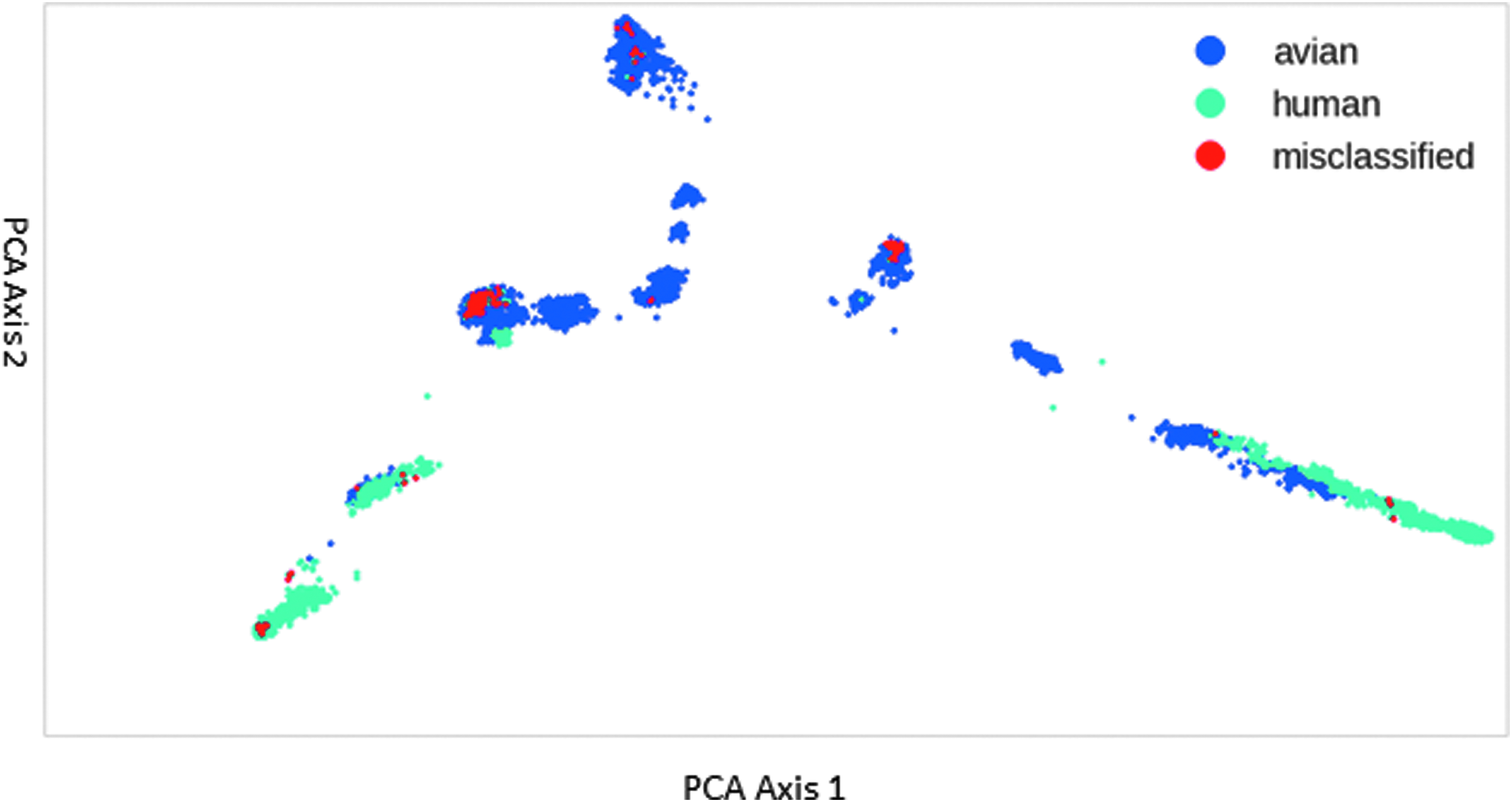
PCA representation of influenza A data for hemagglutinin protein. The X and Y axes are deduced from PCA and are the basis vectors of the covariance matrix corresponding to the largest eigenvalues. Color images are available online.

Visualizations

Every strain is a L × 1 × 26 one-hot encoded tensor. By flattening the array to 1 × L * 26 (1 spot for each of the 26 amino acid symbols), the data are converted into a vector. Principal component analysis (PCA) is a way of reducing the dimensionality of data to its most important components by using matrix factoring.²¹ In this way, PCA reduces the data to a visualizable number of dimensions (eg, 2) while preserving important relationships between data. Figure 3 shows the 2-dimensional PCA representation of HA data, colored by classification.

It was hypothesized that there would be clear clusters of strains by tropism, with a gradient on which strains could be considered “more human” or “more avian.” Instead, there are a number of “islands,” some of which are divided (although not cleanly) between human and avian strains. Different data labeling schemes helped clarify the clusters.

Visualizing the Network Kernels and Responses

To gain insight into what the Tailored CNN end-to-end model is learning from the data, some properties of the model and its response to data samples were examined.

The convolution filter responses were visualized. In this approach, the response is inspected after passing the input data through one particular (generally the first) convolutional layer.²² Each point in each filter has a higher value if the convolution over that area is more salient for classification. In this experiment, each point n on the input has a higher value if it and the 2 surrounding points (because the convolution filter is of size 3) are deemed “more salient” for classification later in the network. The goal is to pinpoint some part of the input data that drive the network response. In the context of this experiment, the response can be used to indicate the relative importance of each position in the amino acid sequence. This procedure starts by computing the average response across all data points at the output of the first layer of the network, in order to highlight positions that are most salient despite sample variations in the data. The next step is to take the absolute difference between mean human and avian strain responses in order to remove common elements, theoretically leaving only the differential elements as the ones with the highest response. The average human, avian, and difference responses for a model trained on HA are illustrated for each of the 3 filters.

It is important to note that this system is no more taxing than visualization for previous techniques used (eg, decision trees). To achieve the visualizations, input data are fed into the network as in a forward inference. The only difference is that the endpoint is not the classification layer, but one of the earlier convolutional layers.

At this point, the results yield a list of input amino acid positions that in theory are more important to classification (relative to other input amino acids). One way to test this hypothesis is to remove the top 10 of these amino acid positions as input, note the change in classification cross-entropy loss relative to the original network, and compare with the removal of 10 random amino acid positions. To ensure that other factors, such as differences between strains, do not influence the outcome, the H1N1 virus subset was examined (see Table 3).

Table 3.

Increased Loss from Blocking Out the Top Responding Spots for H1N1 Inputs

Input Blocking Method	Cross Entropy Loss
None	0.008
Random spots	0.019
Top response spots	0.0067

These results indicate that the most critical amino acid positions derived from this method do indeed play an outsized role in host tropism prediction. The experiment was also repeated with all strains (see Table 4). Note that for this experiment, 50 amino acid input positions were blocked (as opposed to 10 in Table 3) in order to see a noticeable effect on the loss. This shows evidence that different strains have different input positions that are important to host tropism.

Table 4.

Increased Loss from Blocking Out the Top 50 Responding Spots for All Strains

Input Blocking Method	Cross Entropy Loss
None	0.04
Random spots	0.13
Top response spots	0.26

Highlighting “Important” Amino Acids on 3D Protein Models

Influenza HA binds to sialic acid (SA)–containing receptors on target cells. HA host receptor binding specificity is known to be a critical determinant of influenza host specificity.²³ In general, avian strains tend to have HA with affinity for glycan receptors terminating in α2,3-linked SA, while mammalian-adapted strains have HA with higher affinity for glycan receptors terminating in α2,6-linked SA. The glycan receptor-binding site (RBS) of HA is a shallow pocket at the tip of the protein framed by an α-helix at the top (190 helix) and 2 loops at the side (220 loop) and bottom (130 loop).²⁴ Residues in these regions have been associated with glycan receptor affinity, which have a direct impact on host specificity. For instance, in H1 isolates, changes to residues 190 and 225 have been shown to be responsible for the switch between avian and human type receptor specificity.^25,26 These also affect the host receptor specificity of H2 and H3 HAs.²⁷ Importantly, each region of the HA RBS was identified by the CNN as important for classification of influenza human versus avian tropism. The specific critical residues for classification included 131-2, 190-1, and 225-6. Other subunit 1 residues designated as important for classification by the CNN (illustrated in Figure 4) include 54, 59, 67, 76, 78, 88, 120, 183, 239, 254, 261, 298, and 305. Protein structures were downloaded from the Protein Data Bank.²⁸ Visualizing the locations of these amino acids within the 3-dimensional HA protein structure necessitated mapping them onto available PDB structures of the proteins. Specifically, 4GXX, which is from a 1918 strain of avian flu, was chosen. Note that this study used high-resolution structures that included most of the protein. Figure 5 shows the residues critical for CNN classification overlaid on the HA structure 4GXX. Aside from the residues found within the RBS, the other salient residues identified by the CNN have not been previously noted as being critical for host specificity via effects on receptor binding, glycosylation, or pH of activation. One possibility is that these may be important for the structural architecture of the RBS, which can indirectly affect host specificity and affect the favorability of RBS mutations.

Figure 4.

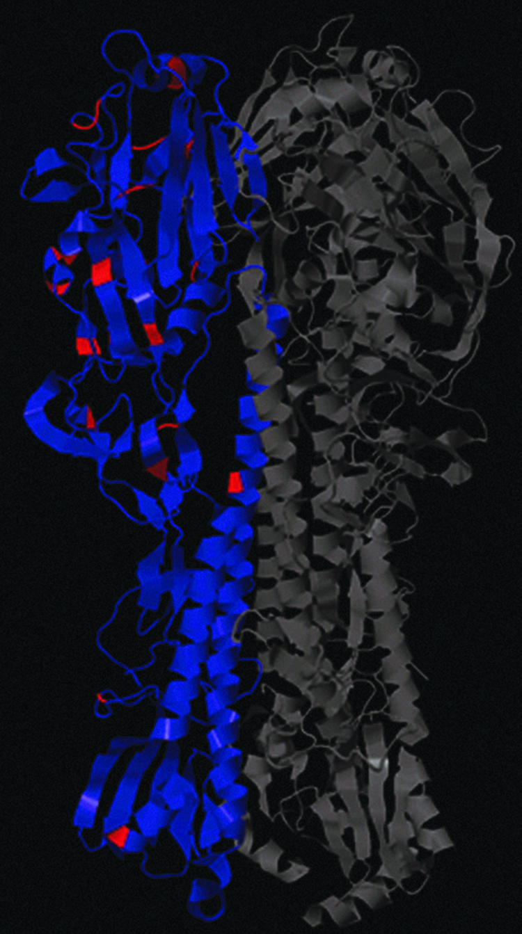
PDB HA structure 4GXX with the most salient amino acids highlighted in red and all other A and B chain residues colored blue. Color images are available online.

Figure 5.

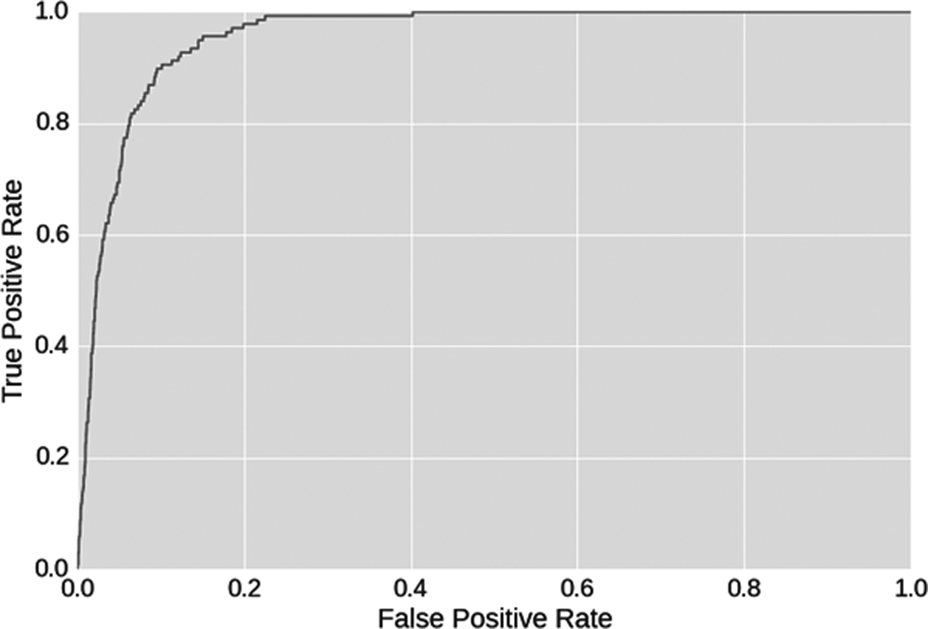
ROC for detecting zoonotic agents from avian strains.

In summary, since the CNN performs end-to-end learning on the amino acid sequence, it “learns” which amino acids in which locations are most important to classification. It is expected that higher layers in the network encode more sophisticated patterns, such as specific amino acid subsequences important to tropism. Other network analysis experiments might be able to extract more information about the role specific amino acid sequences play in viral tropism.

Application: Detecting Avian Strains Likely to Infect Humans

When a previously unseen strain is sampled from an animal host, it is important to quickly determine whether the strain may be zoonotic. This can allow public health officials to predict and intercept potential human outbreaks.^1-3 The following experiment simulates this potential use case and thus illustrates the practical use of the system.

Viral samples of interest (those with potential to cross hosts) were taken from the test data set. Specifically, strains that were isolated from both human and avian hosts were extracted. Then these were combined with the avian-only strains of the test set. This produces a dataset with 137 positive data samples for cross-host infection and 7,820 negative (avian) ones. The softmax of the end layer of the network (confidence the classifier has that a point is human) is used for scoring the strains by the classifier. Softmax is a normalizing operation used in deep neural networks to convert the end layer of the network in a probability distribution across potential hosts.²⁹ The predictive capability of the system is quantified in a receiver operating characteristic (ROC) (Figure 5).

The results indicate that over 90% of all positive samples can be found with only a 10% false alarm rate, and nearly all positive strains can be detected with a 20% false alarm rate. The experimental results demonstrate that CNN classifiers can be used as effective zoonotic strain detectors for influenza virus strains.

Discussion

These experiments show that deep CNNs perform well for the problem of influenza virus tropism classification. Deep CNNs save human time and energy by tuning their own features, and they even slightly outperform other machine learning algorithms for this task. As the influenza database continues to increase over time, the CNN can be updated to further improve performance. The features learned by this network also have the potential to be used in other classifiers for similar problems. Also known as transfer learning, this process would also allow for other classifiers to leverage the information learned by this one.

This method also allows users to inspect the neural network to gain insight into the most important amino acids for tropism. As these experiments show, the network is able to learn the importance of certain spots in the sequence with respect to host tropism. In essence, this network is able to guide research into the causes of viral tropism, and by analyzing the responses of the network to data inputs, simple analysis can distill this implicitly learned information.

This ability could be quite useful for future experimentation. For example, while influenza is known to be amphotropic (broad host tropism), insufficient data exist on the species tropism of virus strains. Currently, the virulence of new virus strains is unknown. Leveraging similarity of new strains to past circulating strains, machine learning methods may be able to estimate viral virulence. Predictions on viral pathogenesis and tissue tropism may be possible by leveraging viral envelope binding interactions with cell receptors and tissue distributions of these receptors. Future experimentation can refine this process, and it is certain that more implicit information can be teased out of these networks in the future.

Lastly, we must note the limitations of our analysis. We assumed that all strains were independent, but the strains themselves were often related evolutionarily. The fact that PCA correlates with phenotype is evidence of nonzero covariance (and thus correlation) between strain proteins, and that the H1N1 restricted analysis selected different predictors, suggests that the classification system is learning to make decisions from lineage, and not just tropism. In this same vein, it is also important to note that the strain classifier performed very well relative to the deep learning classifier. This presents 2 concrete limitations to the analysis. First, the markers found in our analysis might not have a direct biological role to the viral phenotype. Second, the predictive capabilities on strains of unknown lineages may be poorer than on known ones.

Footnotes

Acknowledgments

We would like to thank Peter Carr, Brian Telfer, and Edward Wack for advising this project and providing essential guidance in biology and virology. This material is based upon work supported under Air Force Contract No. FA8721-05-C-0002 and/or FA8702-15-D-0001. Any opinions, findings, conclusions or recommendations expressed in this material are those of the author(s) and do not necessarily reflect the views of the U.S. Air Force.

References

Eng

, Tong

, Tan

. Distinct host tropism protein signatures to identify possible zoonotic influenza A viruses. PLoS One, 2016; 11(2):e0150173.

Eng

, Tong

, Tan

. Predicting host tropism of influenza A virus proteins using random forest. BMC Med Genomics, 2014; 7(Suppl 3): S1.

Alipanahi

, Delong

, Weirauch

, Frey

. Predicting the sequence specificities of DNA- and RNA-binding proteins by deep learning. Nat Biotechnol, 2015; 33(8):831-838.

Yang

, Sugimoto

, Halloran

, et al. The transmissibility and control of pandemic influenza A (H1N1) virus. Science, 2009; 326(5953):729-733.

Howden

, Brockoff

, Caya

, et al. An investigation into human pandemic influenza virus (H1N1) 2009 on an Alberta swine farm. Can Vet J, 2009; 50(11):1153-1161.

Stein

RA.

Lessons from outbreaks of H1N1 influenza. Ann Intern Med, 2009; 151(1):59-62.

Webster

, Bean

, Gorman

, Chambers

, Kawaoka

. Evolution and ecology of influenza A viruses. Microbiol Rev, 1992; 56(1):152-179.

Krizhevsky

, Sutskever

, Hinton

. ImageNet classification with deep convolutional neural networks. In: Advances in Neural Information Processing Systems 25. 2012. https://papers.nips.cc/paper/4824-imagenet-classification-with-deep-convolutional-neural-networks.pdf. Accessed October 30, 2019.

LeCun

, Bottou

, Bengio

, Haffner

Gradient-based learning applied to document recognition. Proc IEEE, 1998:2278-2324.

10.

Szegedy

, Liu

, Jia

, et al. Going deeper with convolutions. Paper presented at: Conference on Computer Vision and Pattern Recognition; June 7–12, 2015; Boston, MA.

11.

Benson

, Cavanaugh

, Clark

, et al. GenBank. Nucleic Acids Res, 2013; 41(Database issue):D36-D42.

12.

Ricke

https://github.com/doricke/BioTools/tree/master/GenBankParser. Accessed October 30, 2019.

13.

Darrell

, Scherbina

. Dawn: rapid large-scale protein multiple sequence alignment and conservation analysis. Paper presented at: 2015 IEEE High Performance Extreme Computing Conference; September 15–17, 2015; Waltham, MA.

14.

Sievers

, Wilm

, Dineen

, et al. Fast, scalable generation of high-quality protein multiple sequence alignments using Clustal Omega. Mol Syst Biol, 2011; 7:539.

15.

Jmol: an open-source Java viewer for chemical structures in 3D. http://www.jmol.org/. Accessed October 30, 2019.

16.

Russell

, Haire

, Stevens

, et al. The structure of H5N1 avian influenza neuraminidase suggests new opportunities for drug design. Nature, 2006; 443(7107):45-49.

17.

Tsibane

, Ekiert

, Krause

, et al. Influenza human monoclonal antibody 1F1 interacts with three major antigenic sites and residues mediating human receptor specificity in H1N1 viruses. PLoS Pathog, 2012; 8(12):e1003067.

18.

Miller

, Vandome

, McBrewster

. Levenshtein Distance: Information Theory, Computer Science, String (computer science), String Metric, Damerau? Levenshtein Distance, Spell Checker, Hamming Distance. Alpha Press; 2009.

19.

Simonyan

, Zisserman

. Very deep convolutional networks for large-scale image recognition. arXiv preprint arXiv:1409.1556. 2014.

20.

Ioffe

, Szegedy

Batch normalization: accelerating deep network training by reducing internal covariate shift. In: Proceedings of the 32nd International Conference on Machine Learning; Brookline, MA: Microtome Publishing; 2015:448-456.

21.

Wold

, Esbensen

, Geladi

Principal component analysis. Chemometr Intell Lab Syst, 1987:37-52.

22.

Zeiler

, Fergus

Visualizing and understanding convolutional networks. Paper presented at: 13th European Conference on Computer Vision; 2014.

23.

Lipsitch

, Barclay

, Raman

, et al. Viral factors in influenza pandemic risk assessment. Elife, 2016; 5:e18491.

24.

Skehel

, Wiley

. Receptor binding and membrane fusion in virus entry: the influenza hemagglutinin. Annu Rev Biochem, 2000; 69:531-569.

25.

Glaser

, Stevens

, Zamarin

, et al. A single amino acid substitution in 1918 influenza virus hemagglutinin changes receptor binding specificity. J Virol, 2005; 79(17):11533-11536.

26.

, McBride

, Nycholat

, Paulson

, Wilson

. Structural characterization of the hemagglutinin receptor specificity from the 2009 H1N1 influenza pandemic. J Virol, 2012; 86(2):982-990.

27.

Stevens

, Blixt

, Chen

, Donis

, Paulson

, Wilson

. Recent avian H5N1 viruses exhibit increased propensity for acquiring human receptor specificity. J Mol Biol, 2008; 381(5):1382-1394.

28.

Berman

, Westbrook

, Feng

, et al. The protein data bank. Nucleic Acids Res, 2000; 28(1):235-242.

29.

Bishop

CM.

Pattern Recognition and Machine Learning. New York: Springer-Verlag; 2006.

30.

Schrauwen

, Fouchier

. Host adaptation and transmission of influenza A viruses in mammals. Emerg Microbes Infect, 2014; 3(2):e9.