Modeling and Simulation of Substrate and Product Inhibitions of Fermentation of Cassava ( Manihot Esculenta ) Extract

Abstract

The fermentation of cassava extracts in brewing is often hampered by microbial inhibitors and oscillations from product and substrate inhibitions, which often decrease ethanol yields. Previous evaluation of the modeling of ethanol inhibition during fermentation of cassava extracts showed low model accuracy. This low model accuracy is due to substrate inhibition, which increases process control challenges. The inhibition patterns considered in this work were linear, sudden growth stop, and exponential. Mathematical models were developed to simulate substrate and product inhibitions during the fermentation of cassava extracts for alcohol production. The results obtained showed substrate and product inhibitions exist during fermentation of cassava extracts, with inhibition patterns being linear substrate-exponential product, exponential substrate-exponential product, and linear substrate-linear product inhibitions. The obtained models are described with a high degree of accuracy (99% confidence interval). The developed models thus agree well with experimental data.

Introduction

Fermentation principles consist of exploiting the metabolic reactions that take place in the cell of a microorganism for the production of valuable products.¹ For ethanol fermentation, the three most common yeast strains usually used include: ale yeasts, which are top-fermenting, can ferment at higher temperatures, and tend to produce more esters; lager yeasts, which are bottom fermenting, withstand lower temperatures, and produce a crisper taste; and wild yeasts, which produce a lot of unusual compounds and contribute to a “horse sweat” flavor that is more acidic. In order to activate the metabolic pathways of interest within the cell, specific environmental conditions, namely temperature, pH, and nutrient concentration, are applied to enable the yeast cell to grow and produce ethanol. However, due to the dynamic nature of the culture medium, yeast cells often suffer from various stresses from both the environmental conditions and from product and/or substrate imbibition.

Cassava (Manihot esculenta) is one of the most important food crops in the humid tropics, and its high starch content makes it extremely suitable for alcohol industries seeking a local substitute for imported barley.² Though alcohol production using cassava extracts involves several unit operations, the fermentation step requires near-optimal process conditions for microorganisms to grow, multiply, and produce the desired ethanol quality.³ However, studies regarding bioreactors and cassava extracts have shown that suboptimal conditions resulting from intrinsic microbial inhibitors and oscillations from product and substrate inhibition often affect fermentation performance.^4

–9 These inhibitions increase the residual sugar at the end of the fermentation, decreasing raw material consumption, and correspondingly, the ethanol yield if no economically acceptable attenuation strategies are developed.⁹ In a typical procedure for modeling ethanol fermentation, if inhibition is considered, it is often conventional to predefine the inhibition pattern. However, this practice increases uncertainties in the model since inhibition pattern varies depending on the type of microorganism and on the type and strength of fermentation wort.¹⁰ It also increases the unreliability of process controllers and simulators, since these automatic tools are usually based on a mathematical representation of the considered system.³

In recent years, there has been extensive research to explore locally sourced raw materials as alternatives to barley in brewing to create more affordable beer and more opportunities for local stake holders. Cassava has been among the candidate raw materials, and many breweries are already using it for beer production. However, several studies examining the dynamics of bioreactors have reported oscillations in both aerobic and anaerobic cultures of Saccharomyces cerevisiae; such instability is more complicated in ethanol fermentation systems due to ethanol inhibition and the lag response of yeast cells to this inhibition.^5

–9 Most research geared toward exploring these problems has been qualitative in nature—focusing on the intracellular mechanisms and how they affect cellular growth—and often predefine the mathematical pattern of the inhibition.

This paper therefore describes dynamic models, incorporating the various effects of substrate- and product-inhibition patterns. These models could be helpful in determining optimal control systems that can minimize the effect of such inhibitions during fermentation processes.

Materials and Methods

Kinetics of Growth and Product Formation

Considering the Monod Equation for cell growth and product formation—Equations 1–2—three inhibition patterns were considered in modeling product inhibition. These include linear, sudden growth stop, and exponential as shown in Table 1 . Four inhibition patterns were considered in modeling the kinetics of growth and product formation: Linear Substrate and Linear Product Inhibition Model (LS-LP), Linear Substrate and Exponential Product Inhibition Model (LS-EP), Exponential Substrate and Linear Product Inhibition Model (ES-LP), and Exponential Substrate and Exponential Product Inhibition Model (ES-EP) inhibitions ( Table 2 ). \documentclass{aastex}\usepackage{amsbsy}\usepackage{amsfonts}\usepackage{amssymb}\usepackage{bm}\usepackage{mathrsfs}\usepackage{pifont}\usepackage{stmaryrd}\usepackage{textcomp}\usepackage{portland, xspace}\usepackage{amsmath, amsxtra}\pagestyle{empty}\DeclareMathSizes{10}{9}{7}{6}\begin{document} \begin{align*} \mu \left( S \right) = { \frac { { \mu _ { max } } S } { { K_ { sx } } + S } } \tag { \it Equation \ \it 1} \end{align*} \end{document}

Table 1.

Mathematical Expressions for the Product Inhibition Factors

PRODUCT INHIBITION FACTOR	MATHEMATICAL EXPRESSION
Linear	\documentclass{aastex}\usepackage{amsbsy}\usepackage{amsfonts}\usepackage{amssymb}\usepackage{bm}\usepackage{mathrsfs}\usepackage{pifont}\usepackage{stmaryrd}\usepackage{textcomp}\usepackage{portland, xspace}\usepackage{amsmath, amsxtra}\pagestyle{empty}\DeclareMathSizes{10}{9}{7}{6}\begin{document}$$ ( {1 - {K_2}P} )$$ \end{document}
Sudden growth stop	\documentclass{aastex}\usepackage{amsbsy}\usepackage{amsfonts}\usepackage{amssymb}\usepackage{bm}\usepackage{mathrsfs}\usepackage{pifont}\usepackage{stmaryrd}\usepackage{textcomp}\usepackage{portland, xspace}\usepackage{amsmath, amsxtra}\pagestyle{empty}\DeclareMathSizes{10}{9}{7}{6}\begin{document}$$ \left( { 1 - \frac { P } { { { P_ { max } } } } } \right)$$ \end{document}
Exponential	\documentclass{aastex}\usepackage{amsbsy}\usepackage{amsfonts}\usepackage{amssymb}\usepackage{bm}\usepackage{mathrsfs}\usepackage{pifont}\usepackage{stmaryrd}\usepackage{textcomp}\usepackage{portland, xspace}\usepackage{amsmath, amsxtra}\pagestyle{empty}\DeclareMathSizes{10}{9}{7}{6}\begin{document}$$ {e^{ - {K_1}}}P$$ \end{document}

Table 2.

Mathematical Expressions for the Substrate and Product Inhibition Factors

INHIBITION FACTOR	MATHEMATICAL EXPRESSION
Linear product (LP)	\documentclass{aastex}\usepackage{amsbsy}\usepackage{amsfonts}\usepackage{amssymb}\usepackage{bm}\usepackage{mathrsfs}\usepackage{pifont}\usepackage{stmaryrd}\usepackage{textcomp}\usepackage{portland, xspace}\usepackage{amsmath, amsxtra}\pagestyle{empty}\DeclareMathSizes{10}{9}{7}{6}\begin{document}$$ ( {1 - { K_2} P} )$$ \end{document}
Exponential product (EP)	\documentclass{aastex}\usepackage{amsbsy}\usepackage{amsfonts}\usepackage{amssymb}\usepackage{bm}\usepackage{mathrsfs}\usepackage{pifont}\usepackage{stmaryrd}\usepackage{textcomp}\usepackage{portland, xspace}\usepackage{amsmath, amsxtra}\pagestyle{empty}\DeclareMathSizes{10}{9}{7}{6}\begin{document}$$ ( {{e^{ - {K_ 1}}}P} )$$ \end{document}
Linear substrate (LS)	\documentclass{aastex}\usepackage{amsbsy}\usepackage{amsfonts}\usepackage{amssymb}\usepackage{bm}\usepackage{mathrsfs}\usepackage{pifont}\usepackage{stmaryrd}\usepackage{textcomp}\usepackage{portland, xspace}\usepackage{amsmath, amsxtra}\pagestyle{empty}\DeclareMathSizes{10}{9}{7}{6}\begin{document}$$ ( 1 - {K_2}S )$$ \end{document}
Exponential substrate (ES)	\documentclass{aastex}\usepackage{amsbsy}\usepackage{amsfonts}\usepackage{amssymb}\usepackage{bm}\usepackage{mathrsfs}\usepackage{pifont}\usepackage{stmaryrd}\usepackage{textcomp}\usepackage{portland, xspace}\usepackage{amsmath, amsxtra}\pagestyle{empty}\DeclareMathSizes{10}{9}{7}{6}\begin{document}$$ ( {{e^{ - {K_1}}}S} )$$ \end{document}

where \documentclass{aastex}\usepackage{amsbsy}\usepackage{amsfonts}\usepackage{amssymb}\usepackage{bm}\usepackage{mathrsfs}\usepackage{pifont}\usepackage{stmaryrd}\usepackage{textcomp}\usepackage{portland, xspace}\usepackage{amsmath, amsxtra}\pagestyle{empty}\DeclareMathSizes{10}{9}{7}{6}\begin{document}$${ \mu _{max}}$$ \end{document} is the maximum specific growth rate (h⁻¹) and \documentclass{aastex}\usepackage{amsbsy}\usepackage{amsfonts}\usepackage{amssymb}\usepackage{bm}\usepackage{mathrsfs}\usepackage{pifont}\usepackage{stmaryrd}\usepackage{textcomp}\usepackage{portland, xspace}\usepackage{amsmath, amsxtra}\pagestyle{empty}\DeclareMathSizes{10}{9}{7}{6}\begin{document}$${K_{sx}}$$ \end{document} is the substrate saturation (Monod) constant for cell growth (g/100 g). \documentclass{aastex}\usepackage{amsbsy}\usepackage{amsfonts}\usepackage{amssymb}\usepackage{bm}\usepackage{mathrsfs}\usepackage{pifont}\usepackage{stmaryrd}\usepackage{textcomp}\usepackage{portland, xspace}\usepackage{amsmath, amsxtra}\pagestyle{empty}\DeclareMathSizes{10}{9}{7}{6}\begin{document} \begin{align*}{ q_p } \left( S \right) = { \frac { { q_ { pmax } } S } { { K_ { sp } } + S } } \tag { \it Equation \ \it 2} \end{align*} \end{document}

Substrate and Product Inhibition Models

By incorporating the effect of substrate and product inhibitions into the Monod equation and using the inhibition factors in Table 1 , the following kinetic models were obtained:

▪ Kinetics with linear substrate and linear product inhibitions \documentclass{aastex}\usepackage{amsbsy}\usepackage{amsfonts}\usepackage{amssymb}\usepackage{bm}\usepackage{mathrsfs}\usepackage{pifont}\usepackage{stmaryrd}\usepackage{textcomp}\usepackage{portland, xspace}\usepackage{amsmath, amsxtra}\pagestyle{empty}\DeclareMathSizes{10}{9}{7}{6}\begin{document} \begin{align*} \mu \left( { S,P } \right) = \left( { 1 - { K_ { ix } } P } \right) \left( { 1 - { K_ { isx } } S } \right) { \frac { { \mu _{ max } } S } { { K_ { sx } } + S } } \tag {{\it Equation \ \it 3} } \end{align*} \end{document}

where \documentclass{aastex}\usepackage{amsbsy}\usepackage{amsfonts}\usepackage{amssymb}\usepackage{bm}\usepackage{mathrsfs}\usepackage{pifont}\usepackage{stmaryrd}\usepackage{textcomp}\usepackage{portland, xspace}\usepackage{amsmath, amsxtra}\pagestyle{empty}\DeclareMathSizes{10}{9}{7}{6}\begin{document}$${K_{ix}}$$ \end{document} is product inhibition coefficient on cell growth and \documentclass{aastex}\usepackage{amsbsy}\usepackage{amsfonts}\usepackage{amssymb}\usepackage{bm}\usepackage{mathrsfs}\usepackage{pifont}\usepackage{stmaryrd}\usepackage{textcomp}\usepackage{portland, xspace}\usepackage{amsmath, amsxtra}\pagestyle{empty}\DeclareMathSizes{10}{9}{7}{6}\begin{document}$${K_{isx}}$$ \end{document} is substrate inhibition coefficient on cell growth. \documentclass{aastex}\usepackage{amsbsy}\usepackage{amsfonts}\usepackage{amssymb}\usepackage{bm}\usepackage{mathrsfs}\usepackage{pifont}\usepackage{stmaryrd}\usepackage{textcomp}\usepackage{portland, xspace}\usepackage{amsmath, amsxtra}\pagestyle{empty}\DeclareMathSizes{10}{9}{7}{6}\begin{document} \begin{align*} q \left( { S,P } \right) = \left( { 1 - { K_ { ip } } P } \right) \left( { 1 - { K_ { isx } } S } \right) { \frac { { q_ { max } } S} { { K_ { sx } } + S } } \tag {{\it Equation \ \it 4}} \end{align*} \end{document}

▪Kinetics with linear substrate and exponential product inhibitions \documentclass{aastex}\usepackage{amsbsy}\usepackage{amsfonts}\usepackage{amssymb}\usepackage{bm}\usepackage{mathrsfs}\usepackage{pifont}\usepackage{stmaryrd}\usepackage{textcomp}\usepackage{portland, xspace}\usepackage{amsmath, amsxtra}\pagestyle{empty}\DeclareMathSizes{10}{9}{7}{6}\begin{document} \begin{align*} \mu \left( { S,P } \right) = \left( { 1 - { K_ { isx } } S } \right) exp \left( { - { K_ { ix } } P } \right) { \frac { { \mu _{ max } } S } { { K_ { sx } } + S } } \tag {{\it Equation \ \it 5}} \end{align*} \end{document} \documentclass{aastex}\usepackage{amsbsy}\usepackage{amsfonts}\usepackage{amssymb}\usepackage{bm}\usepackage{mathrsfs}\usepackage{pifont}\usepackage{stmaryrd}\usepackage{textcomp}\usepackage{portland, xspace}\usepackage{amsmath, amsxtra}\pagestyle{empty}\DeclareMathSizes{10}{9}{7}{6}\begin{document} \begin{align*} q \left( { S,P } \right) = \left( { 1 - { K_ { isp } } S } \right) exp \left( { - { K_ { ip } } P } \right) { \frac { { q_ { max } } S } { { K_ { sx } } + S } } \tag {{\it Equation \ \it 6}} \end{align*} \end{document}

▪ Kinetics with exponential substrate and linear product inhibitions \documentclass{aastex}\usepackage{amsbsy}\usepackage{amsfonts}\usepackage{amssymb}\usepackage{bm}\usepackage{mathrsfs}\usepackage{pifont}\usepackage{stmaryrd}\usepackage{textcomp}\usepackage{portland, xspace}\usepackage{amsmath, amsxtra}\pagestyle{empty}\DeclareMathSizes{10}{9}{7}{6}\begin{document} \begin{align*} \mu \left( { S,P } \right) = \left( { 1 - { K_ { ix } } P } \right) exp \left( { - { K_ { isx } } S } \right) { \frac { { \mu _ { max } } S } { { K_m } + S } } \tag {{\it Equation \ \it 7}} \end{align*} \end{document} \documentclass{aastex}\usepackage{amsbsy}\usepackage{amsfonts}\usepackage{amssymb}\usepackage{bm}\usepackage{mathrsfs}\usepackage{pifont}\usepackage{stmaryrd}\usepackage{textcomp}\usepackage{portland, xspace}\usepackage{amsmath, amsxtra}\pagestyle{empty}\DeclareMathSizes{10}{9}{7}{6}\begin{document} \begin{align*} q \left( { S,P } \right) = \left( { 1 - pP } \right) exp \left( {- { K_ { isp } } S } \right) { \frac { { q_ { max } } S } { { K_m} + S } } \tag {{\it Equation \ \it 8}} \end{align*} \end{document}

▪ Kinetics with exponential substrate and exponential product inhibitions \documentclass{aastex}\usepackage{amsbsy}\usepackage{amsfonts}\usepackage{amssymb}\usepackage{bm}\usepackage{mathrsfs}\usepackage{pifont}\usepackage{stmaryrd}\usepackage{textcomp}\usepackage{portland, xspace}\usepackage{amsmath, amsxtra}\pagestyle{empty}\DeclareMathSizes{10}{9}{7}{6}\begin{document} \begin{align*} \mu \left( { S,P } \right) = exp \left( { - { K_ { ix } } P } \right) { \frac { { \mu _ { max } } S } { { K_ { sx } } + S } } exp \left( { - { K_ { isx } } S } \right) \tag {{\it Equation \ \it 9}} \end{align*} \end{document} \documentclass{aastex}\usepackage{amsbsy}\usepackage{amsfonts}\usepackage{amssymb}\usepackage{bm}\usepackage{mathrsfs}\usepackage{pifont}\usepackage{stmaryrd}\usepackage{textcomp}\usepackage{portland, xspace}\usepackage{amsmath, amsxtra}\pagestyle{empty}\DeclareMathSizes{10}{9}{7}{6}\begin{document} \begin{align*} q \left( { S,P } \right) = exp \left( { - { K_ { ip } } P } \right) { \frac { { q_ { max } } S } { { K_ { sp } } + S } } exp \left( { - { K_ { isp } } S } \right) \tag {{\it Equation \ \it 10}} \end{align*} \end{document}

Introducing the effect of product inhibition into the Monod equation, and using the respective inhibition factors, yielded the following kinetic models:

▪ Kinetics with linear product inhibition (also known as the Hinshelwood-Dagley model)¹¹ \documentclass{aastex}\usepackage{amsbsy}\usepackage{amsfonts}\usepackage{amssymb}\usepackage{bm}\usepackage{mathrsfs}\usepackage{pifont}\usepackage{stmaryrd}\usepackage{textcomp}\usepackage{portland, xspace}\usepackage{amsmath, amsxtra}\pagestyle{empty}\DeclareMathSizes{10}{9}{7}{6}\begin{document} \begin{align*} \mu \left( { S,P } \right) = \left( { 1 - { K_ { ix } } P } \right) { \frac { { \mu _ { max } } S } { { K_ { sx } } + S } } \tag {{\it Equation \ \it 11}} \end{align*} \end{document} \documentclass{aastex}\usepackage{amsbsy}\usepackage{amsfonts}\usepackage{amssymb}\usepackage{bm}\usepackage{mathrsfs}\usepackage{pifont}\usepackage{stmaryrd}\usepackage{textcomp}\usepackage{portland, xspace}\usepackage{amsmath, amsxtra}\pagestyle{empty}\DeclareMathSizes{10}{9}{7}{6}\begin{document} \begin{align*} q \left( { S,P } \right) = \left( { 1 - { K_ { ip } } P } \right){ \frac { { q_ { max } } S } { { K_ { sx } } + S } } \tag {{\it Equation \ \it 12}} \end{align*} \end{document}

▪ Kinetics sudden growth stop product inhibition (also known as Ghose-Tyagi model)¹² \documentclass{aastex}\usepackage{amsbsy}\usepackage{amsfonts}\usepackage{amssymb}\usepackage{bm}\usepackage{mathrsfs}\usepackage{pifont}\usepackage{stmaryrd}\usepackage{textcomp}\usepackage{portland, xspace}\usepackage{amsmath, amsxtra}\pagestyle{empty}\DeclareMathSizes{10}{9}{7}{6}\begin{document} \begin{align*} \mu \left( { S,P } \right) = \left( { 1 - \frac { P } { { { P_ { pmax } } } } } \right) { \frac { { \mu_ { max } } S } { { K_ { sx} } + S } } \tag {{\it Equation \ \it 13}} \end{align*} \end{document} \documentclass{aastex}\usepackage{amsbsy}\usepackage{amsfonts}\usepackage{amssymb}\usepackage{bm}\usepackage{mathrsfs}\usepackage{pifont}\usepackage{stmaryrd}\usepackage{textcomp}\usepackage{portland, xspace}\usepackage{amsmath, amsxtra}\pagestyle{empty}\DeclareMathSizes{10}{9}{7}{6}\begin{document} \begin{align*} q \left( { S,P } \right) = \left( { 1 - \frac { P } { { { P_ { pmax } } } } } \right) { \frac { { q_ { max } } S } { { K_ { sx }} + S } } \tag {{\it Equation \ \it 14}} \end{align*} \end{document}

▪ Kinetics with exponential product inhibition (also known as the Aiba and Shoda model)¹³ \documentclass{aastex}\usepackage{amsbsy}\usepackage{amsfonts}\usepackage{amssymb}\usepackage{bm}\usepackage{mathrsfs}\usepackage{pifont}\usepackage{stmaryrd}\usepackage{textcomp}\usepackage{portland, xspace}\usepackage{amsmath, amsxtra}\pagestyle{empty}\DeclareMathSizes{10}{9}{7}{6}\begin{document} \begin{align*} \mu \left( { S,P } \right) = exp \left( { - { K_ { ix } } P } \right) { \frac { { \mu _ { max } } S } { { K_ { sx } } + S } } \tag {{\it Equation \ \it 15}} \end{align*} \end{document} \documentclass{aastex}\usepackage{amsbsy}\usepackage{amsfonts}\usepackage{amssymb}\usepackage{bm}\usepackage{mathrsfs}\usepackage{pifont}\usepackage{stmaryrd}\usepackage{textcomp}\usepackage{portland, xspace}\usepackage{amsmath, amsxtra}\pagestyle{empty}\DeclareMathSizes{10}{9}{7}{6}\begin{document} \begin{align*} q \left( { S,P } \right) = exp \left( { - { K_ { ip } } P } \right) { \frac { { q_ { max } } S } { { K_ { sx } } + S } } \tag{{\it Equation \ \it 16}} \end{align*} \end{document}

Material Balance and Development of Differential Equations

The ordinary differential equations that describe cell growth, product formation, and substrate utilization are presented in Equations 16 –18: \documentclass{aastex}\usepackage{amsbsy}\usepackage{amsfonts}\usepackage{amssymb}\usepackage{bm}\usepackage{mathrsfs}\usepackage{pifont}\usepackage{stmaryrd}\usepackage{textcomp}\usepackage{portland, xspace}\usepackage{amsmath, amsxtra}\pagestyle{empty}\DeclareMathSizes{10}{9}{7}{6}\begin{document} \begin{align*}{ \frac { dX } { dt } } = \mu X \tag {{\it Equation \ \it 16A}} \end{align*} \end{document} \documentclass{aastex}\usepackage{amsbsy}\usepackage{amsfonts}\usepackage{amssymb}\usepackage{bm}\usepackage{mathrsfs}\usepackage{pifont}\usepackage{stmaryrd}\usepackage{textcomp}\usepackage{portland, xspace}\usepackage{amsmath, amsxtra}\pagestyle{empty}\DeclareMathSizes{10}{9}{7}{6}\begin{document} \begin{align*}{ \frac { dP } { dt } } = q X \tag {{\it Equation \ \it 17}} \end{align*} \end{document} \documentclass{aastex}\usepackage{amsbsy}\usepackage{amsfonts}\usepackage{amssymb}\usepackage{bm}\usepackage{mathrsfs}\usepackage{pifont}\usepackage{stmaryrd}\usepackage{textcomp}\usepackage{portland, xspace}\usepackage{amsmath, amsxtra}\pagestyle{empty}\DeclareMathSizes{10}{9}{7}{6}\begin{document} \begin{align*}{ \frac { dS } { dt } } = - \frac { 1 } { { { Y_x } } } { \frac { dX } { dt } } - \frac { 1 } { { { Y_p } } } { \frac { dP} { dt } } - { G_s } X - { M_s } X \tag {{\it Equation \ \it 18}} \end{align*} \end{document}

where G_s is the yield coefficient of the cell based on substrate utilization (g/g·h); M_s is the cell growth coefficient on substrate (g/g·h); Y_x is the yield coefficient of the cell based on substrate utilization (g/g); and Y_p is the yield coefficient of the cell based on substrate utilization (g/g).

Using the batch kinetic models Equations 15 and 16, and substituting \documentclass{aastex}\usepackage{amsbsy}\usepackage{amsfonts}\usepackage{amssymb}\usepackage{bm}\usepackage{mathrsfs}\usepackage{pifont}\usepackage{stmaryrd}\usepackage{textcomp}\usepackage{portland, xspace}\usepackage{amsmath, amsxtra}\pagestyle{empty}\DeclareMathSizes{10}{9}{7}{6}\begin{document}$$\mu$$ \end{document} and q in Equations 16 –18 with each of their product-inhibition expressions, the approximate representation of the fermentation process in each inhibition scenario could be described by the following Equations 19 –21:

▪ Dynamics with linear substrate and linear product inhibitions \documentclass{aastex}\usepackage{amsbsy}\usepackage{amsfonts}\usepackage{amssymb}\usepackage{bm}\usepackage{mathrsfs}\usepackage{pifont}\usepackage{stmaryrd}\usepackage{textcomp}\usepackage{portland, xspace}\usepackage{amsmath, amsxtra}\pagestyle{empty}\DeclareMathSizes{10}{9}{7}{6}\begin{document} \begin{align*}{ \frac { dX } { dt } } = \left( { 1 - { K_ { ix } } P } \right) \left( { 1 - { K_ { isx } } S } \right) { \frac { { \mu _{ max } } S } { { K_ { sx } } + S } } X \tag {{\it Equation \ \it 19}} \end{align*} \end{document} \documentclass{aastex}\usepackage{amsbsy}\usepackage{amsfonts}\usepackage{amssymb}\usepackage{bm}\usepackage{mathrsfs}\usepackage{pifont}\usepackage{stmaryrd}\usepackage{textcomp}\usepackage{portland, xspace}\usepackage{amsmath, amsxtra}\pagestyle{empty}\DeclareMathSizes{10}{9}{7}{6}\begin{document} \begin{align*}{ \frac { dP } { dt } } = \left( { 1 - { K_ { ip } } P } \right) \left( { 1 - { K_ { isp } } S } \right) { \frac { { q_ { max } } S } { { K_ { sp } } + S } } X \tag {{\it Equation \ \it 20}} \end{align*} \end{document} \documentclass{aastex}\usepackage{amsbsy}\usepackage{amsfonts}\usepackage{amssymb}\usepackage{bm}\usepackage{mathrsfs}\usepackage{pifont}\usepackage{stmaryrd}\usepackage{textcomp}\usepackage{portland, xspace}\usepackage{amsmath, amsxtra}\pagestyle{empty}\DeclareMathSizes{10}{9}{7}{6}\begin{document} \begin{align*}{ \frac { dS } { dt } } = - \frac { 1 } { { { Y_x } } } { \frac { dX } { dt } } - \frac { 1 } { { { Y_p } } } { \frac { dP } { dt } } - { G_s } X - { M_s } X \tag {{\it Equation \ \it 21}} \end{align*} \end{document}

▪ Dynamics with linear substrate and exponential product inhibition \documentclass{aastex}\usepackage{amsbsy}\usepackage{amsfonts}\usepackage{amssymb}\usepackage{bm}\usepackage{mathrsfs}\usepackage{pifont}\usepackage{stmaryrd}\usepackage{textcomp}\usepackage{portland, xspace}\usepackage{amsmath, amsxtra}\pagestyle{empty}\DeclareMathSizes{10}{9}{7}{6}\begin{document} \begin{align*}{ \frac { dX } { dt } } { = } \left( { 1 - { K_ { isx } } S } \right) exp \left( { - { K_ { ix } } P } \right) { \frac { { \mu _ { max } } S } { { K_ { sx } } + S } } X \tag {{\it Equation \ \it 22}} \end{align*} \end{document} \documentclass{aastex}\usepackage{amsbsy}\usepackage{amsfonts}\usepackage{amssymb}\usepackage{bm}\usepackage{mathrsfs}\usepackage{pifont}\usepackage{stmaryrd}\usepackage{textcomp}\usepackage{portland, xspace}\usepackage{amsmath, amsxtra}\pagestyle{empty}\DeclareMathSizes{10}{9}{7}{6}\begin{document} \begin{align*}{ \frac { dP } { dt } } { = } \left( { 1 - { K_ { isp } } S } \right) exp \left( { - { K_ { ip } } P } \right) { \frac { { q_ { max } } S } { { K_ { sp } } + S } } X \tag {{\it Equation \ \it 23}} \end{align*} \end{document} \documentclass{aastex}\usepackage{amsbsy}\usepackage{amsfonts}\usepackage{amssymb}\usepackage{bm}\usepackage{mathrsfs}\usepackage{pifont}\usepackage{stmaryrd}\usepackage{textcomp}\usepackage{portland, xspace}\usepackage{amsmath, amsxtra}\pagestyle{empty}\DeclareMathSizes{10}{9}{7}{6}\begin{document} \begin{align*}{ \frac { dS } { dt } } = - \frac { 1 } { { { Y_x } } } { \frac { dX } { dt } } - \frac { 1 } { { { Y_p } } } { \frac { dP } { dt } } - { G_s } X - { M_s } X \tag {{\it Equation \ \it 24}} \end{align*} \end{document}

▪ Dynamics with exponential substrate and linear product inhibition \documentclass{aastex}\usepackage{amsbsy}\usepackage{amsfonts}\usepackage{amssymb}\usepackage{bm}\usepackage{mathrsfs}\usepackage{pifont}\usepackage{stmaryrd}\usepackage{textcomp}\usepackage{portland, xspace}\usepackage{amsmath, amsxtra}\pagestyle{empty}\DeclareMathSizes{10}{9}{7}{6}\begin{document} \begin{align*}{ \frac { dX } { dt } } = \left( { 1 - { K_ { ix } } P } \right) exp \left( { - { K_ { isx } } S } \right) { \frac { { \mu _ { max } } S } { { K_ { sx } } + S } } X \tag {{\it Equation \ \it 25}} \end{align*} \end{document} \documentclass{aastex}\usepackage{amsbsy}\usepackage{amsfonts}\usepackage{amssymb}\usepackage{bm}\usepackage{mathrsfs}\usepackage{pifont}\usepackage{stmaryrd}\usepackage{textcomp}\usepackage{portland, xspace}\usepackage{amsmath, amsxtra}\pagestyle{empty}\DeclareMathSizes{10}{9}{7}{6}\begin{document} \begin{align*}{ \frac { dP } { dt } } = \left( { 1 - { K_ { ix } } P } \right) exp \left( { - { K_ { isx } } S } \right) { \frac { { \mu _ { max } } S } { { K_ { sp } } + S } } X \tag {{\it Equation \ \it 26}} \end{align*} \end{document} \documentclass{aastex}\usepackage{amsbsy}\usepackage{amsfonts}\usepackage{amssymb}\usepackage{bm}\usepackage{mathrsfs}\usepackage{pifont}\usepackage{stmaryrd}\usepackage{textcomp}\usepackage{portland, xspace}\usepackage{amsmath, amsxtra}\pagestyle{empty}\DeclareMathSizes{10}{9}{7}{6}\begin{document} \begin{align*}{ \frac { dS } { dt } } = - \frac { 1 } { { { Y_x } } } { \frac { dX } { dt } } - \frac { 1 } { { { Y_p } } } { \frac { dP } { dt } } - { G_s } X - { M_s } X \tag {{\it Equation \ \it 27}} \end{align*} \end{document}

▪ Dynamics with exponential substrate and exponential product inhibitions \documentclass{aastex}\usepackage{amsbsy}\usepackage{amsfonts}\usepackage{amssymb}\usepackage{bm}\usepackage{mathrsfs}\usepackage{pifont}\usepackage{stmaryrd}\usepackage{textcomp}\usepackage{portland, xspace}\usepackage{amsmath, amsxtra}\pagestyle{empty}\DeclareMathSizes{10}{9}{7}{6}\begin{document} \begin{align*}{ \frac { dX } { dt } } = exp \left( { - { K_ { ix } } P } \right) { \frac { { \mu _ { max } } S } { { K_ { sx } } + S } } exp \left( { - { K_ { isx } } S } \right) X \tag { { Equation \ \it 28 } } \end{align*} \end{document} \documentclass{aastex}\usepackage{amsbsy}\usepackage{amsfonts}\usepackage{amssymb}\usepackage{bm}\usepackage{mathrsfs}\usepackage{pifont}\usepackage{stmaryrd}\usepackage{textcomp}\usepackage{portland, xspace}\usepackage{amsmath, amsxtra}\pagestyle{empty}\DeclareMathSizes{10}{9}{7}{6}\begin{document} \begin{align*}{ \frac { dP } { dt } } = exp \left( { - { K_ { ip } } P } \right) { \frac { { q_ { max } } S } { { K_ { sp } } + S } } exp \left( { - { K_ { isp } } S } \right) X \tag {{\it Equation \ \it 29}} \end{align*} \end{document} \documentclass{aastex}\usepackage{amsbsy}\usepackage{amsfonts}\usepackage{amssymb}\usepackage{bm}\usepackage{mathrsfs}\usepackage{pifont}\usepackage{stmaryrd}\usepackage{textcomp}\usepackage{portland, xspace}\usepackage{amsmath, amsxtra}\pagestyle{empty}\DeclareMathSizes{10}{9}{7}{6}\begin{document} \begin{align*}{ \frac { dS } { dt } } = - \frac { 1 } { { { Y_x } } } { \frac { dX } { dt } } - \frac { 1 } { { { Y_p } } } { \frac { dP } { dt } } - { G_s } X - { M_s } X \tag {{\it Equation \ \it 30}} \end{align*} \end{document}

Product Inhibition Models

With the help of batch kinetic models stated above, and substituting \documentclass{aastex}\usepackage{amsbsy}\usepackage{amsfonts}\usepackage{amssymb}\usepackage{bm}\usepackage{mathrsfs}\usepackage{pifont}\usepackage{stmaryrd}\usepackage{textcomp}\usepackage{portland, xspace}\usepackage{amsmath, amsxtra}\pagestyle{empty}\DeclareMathSizes{10}{9}{7}{6}\begin{document}$$\mu$$ \end{document} and q with each of their product-inhibition expressions, the approximate representation of the fermentation process in each inhibition model could be described by the following differential equations:

▪ Dynamics with linear product inhibitions \documentclass{aastex}\usepackage{amsbsy}\usepackage{amsfonts}\usepackage{amssymb}\usepackage{bm}\usepackage{mathrsfs}\usepackage{pifont}\usepackage{stmaryrd}\usepackage{textcomp}\usepackage{portland, xspace}\usepackage{amsmath, amsxtra}\pagestyle{empty}\DeclareMathSizes{10}{9}{7}{6}\begin{document} \begin{align*}{ \frac { dX } { dt } } = \left( { 1 - { K_ { ix } } P } \right) { \frac { { \mu _ { max } } S } { { K_ { sx } } + S } } X \tag {{\it Equation \ \it 31}} \end{align*} \end{document} \documentclass{aastex}\usepackage{amsbsy}\usepackage{amsfonts}\usepackage{amssymb}\usepackage{bm}\usepackage{mathrsfs}\usepackage{pifont}\usepackage{stmaryrd}\usepackage{textcomp}\usepackage{portland, xspace}\usepackage{amsmath, amsxtra}\pagestyle{empty}\DeclareMathSizes{10}{9}{7}{6}\begin{document} \begin{align*}{ \frac { dP } { dt } } = \left( { 1 - { K_ { ip } } P } \right) { \frac { { q_ { max } } S } { { K_ { sp } } + S } } X \tag {{\it Equation \ \it 32}} \end{align*} \end{document} \documentclass{aastex}\usepackage{amsbsy}\usepackage{amsfonts}\usepackage{amssymb}\usepackage{bm}\usepackage{mathrsfs}\usepackage{pifont}\usepackage{stmaryrd}\usepackage{textcomp}\usepackage{portland, xspace}\usepackage{amsmath, amsxtra}\pagestyle{empty}\DeclareMathSizes{10}{9}{7}{6}\begin{document} \begin{align*}{ \frac { dS } { dt } } = - \frac { 1 } { { { Y_x } } } { \frac { dX } { dt } } - \frac { 1 } { { { Y_p } } } { \frac { dP} { dt } } - { G_s } X - { M_s } X \tag {{\it Equation \ \it 33}} \end{align*} \end{document}

▪ Dynamics with sudden growth stop product inhibitions \documentclass{aastex}\usepackage{amsbsy}\usepackage{amsfonts}\usepackage{amssymb}\usepackage{bm}\usepackage{mathrsfs}\usepackage{pifont}\usepackage{stmaryrd}\usepackage{textcomp}\usepackage{portland, xspace}\usepackage{amsmath, amsxtra}\pagestyle{empty}\DeclareMathSizes{10}{9}{7}{6}\begin{document} \begin{align*}{ \frac { dX } { dt } } = \left( { 1 - \frac { P } { { { P_ { max } } } } } \right) { \frac { { \mu _ { max } } S } { { K_ { sx} } + S } } X \tag {{\it Equation \ \it 34}} \end{align*} \end{document} \documentclass{aastex}\usepackage{amsbsy}\usepackage{amsfonts}\usepackage{amssymb}\usepackage{bm}\usepackage{mathrsfs}\usepackage{pifont}\usepackage{stmaryrd}\usepackage{textcomp}\usepackage{portland, xspace}\usepackage{amsmath, amsxtra}\pagestyle{empty}\DeclareMathSizes{10}{9}{7}{6}\begin{document} \begin{align*}{ \frac { dP } { dt } } = \left( { 1 - \frac { P } { { { P_ { pmax } } } } } \right) { \frac { { q _ { max } } S } { { K_ { sp} } + S } } X \tag {{\it Equation \rm 35}} \end{align*} \end{document} \documentclass{aastex}\usepackage{amsbsy}\usepackage{amsfonts}\usepackage{amssymb}\usepackage{bm}\usepackage{mathrsfs}\usepackage{pifont}\usepackage{stmaryrd}\usepackage{textcomp}\usepackage{portland, xspace}\usepackage{amsmath, amsxtra}\pagestyle{empty}\DeclareMathSizes{10}{9}{7}{6}\begin{document} \begin{align*}{ \frac { dS } { dt } } = - \frac { 1 } { { { Y_x } } } { \frac { dX } { dt } } - \frac { 1 } { { { Y_p } } } { \frac { dP } { dt } } - { G_s } X - { M_s } X \tag {{\it Equation \ 36}} \end{align*} \end{document}

▪ Dynamics with exponential product inhibitions \documentclass{aastex}\usepackage{amsbsy}\usepackage{amsfonts}\usepackage{amssymb}\usepackage{bm}\usepackage{mathrsfs}\usepackage{pifont}\usepackage{stmaryrd}\usepackage{textcomp}\usepackage{portland, xspace}\usepackage{amsmath, amsxtra}\pagestyle{empty}\DeclareMathSizes{10}{9}{7}{6}\begin{document} \begin{align*}{ \frac { dX } { dt } } { = } exp \left( { - { K_ { ix } } P } \right) { \frac { { \mu _ { max } } S } { { K_ { sx } } + S } } X \tag {{\it Equation \ 37}} \end{align*} \end{document} \documentclass{aastex}\usepackage{amsbsy}\usepackage{amsfonts}\usepackage{amssymb}\usepackage{bm}\usepackage{mathrsfs}\usepackage{pifont}\usepackage{stmaryrd}\usepackage{textcomp}\usepackage{portland, xspace}\usepackage{amsmath, amsxtra}\pagestyle{empty}\DeclareMathSizes{10}{9}{7}{6}\begin{document} \begin{align*}{ \frac { dP } { dt } } { = } exp \left( { - { K_ { ip } } P } \right) { \frac { { q_ { max } } S } { { K_ { sp } } + S } } X \tag {{\it Equation \ 38}} \end{align*} \end{document} \documentclass{aastex}\usepackage{amsbsy}\usepackage{amsfonts}\usepackage{amssymb}\usepackage{bm}\usepackage{mathrsfs}\usepackage{pifont}\usepackage{stmaryrd}\usepackage{textcomp}\usepackage{portland, xspace}\usepackage{amsmath, amsxtra}\pagestyle{empty}\DeclareMathSizes{10}{9}{7}{6}\begin{document} \begin{align*}{ \frac { dS } { dt } } = - \frac { 1 } { { { Y_x } } } { \frac { dX } { dt } } - \frac { 1 } { { { Y_p } } } { \frac { dP } { dt } } - { G_s } X - { M_s } X \tag {{\it Equation \ 39}} \end{align*} \end{document}

Results and Discussion

Parameter Estimation and Model Validation

The identification of model parameters for the different systems of equations was made with Matlab (Mathworks, Natick, MA), and the ode45 solver was used to simulate the differential equations. This was done by minimizing the overall sum of squared error using Equation 40 between the model simulation and experimental data points of the process variables (Biomass (X), Substrate (S) and Product (P)). \documentclass{aastex}\usepackage{amsbsy}\usepackage{amsfonts}\usepackage{amssymb}\usepackage{bm}\usepackage{mathrsfs}\usepackage{pifont}\usepackage{stmaryrd}\usepackage{textcomp}\usepackage{portland, xspace}\usepackage{amsmath, amsxtra}\pagestyle{empty}\DeclareMathSizes{10}{9}{7}{6}\begin{document} \begin{align*} \varepsilon = \min \sum { [ \left( {X ( {k_1},{k_2}, \ldots ,{k_n}} \right) - {X^e} ) ^2} \\ + \left( {S ( {k_1},{k_2}, \ldots, {k_n}} \right) - {S^e}{ ) ^2} + \left( {P ( {k_1},{k_2}, \ldots, {k_n}} \right) - {P^e}{ ) ^2} ] \end{align*} \end{document}

The model parameters were estimated, and the capability of the mathematical model to describe the fermentation process was tested statistically using the F–tests. This was done using STATA (StataCorp, College Station, TX) at a confidence interval of 99%, to find out the confidence level for the developed mathematical model.

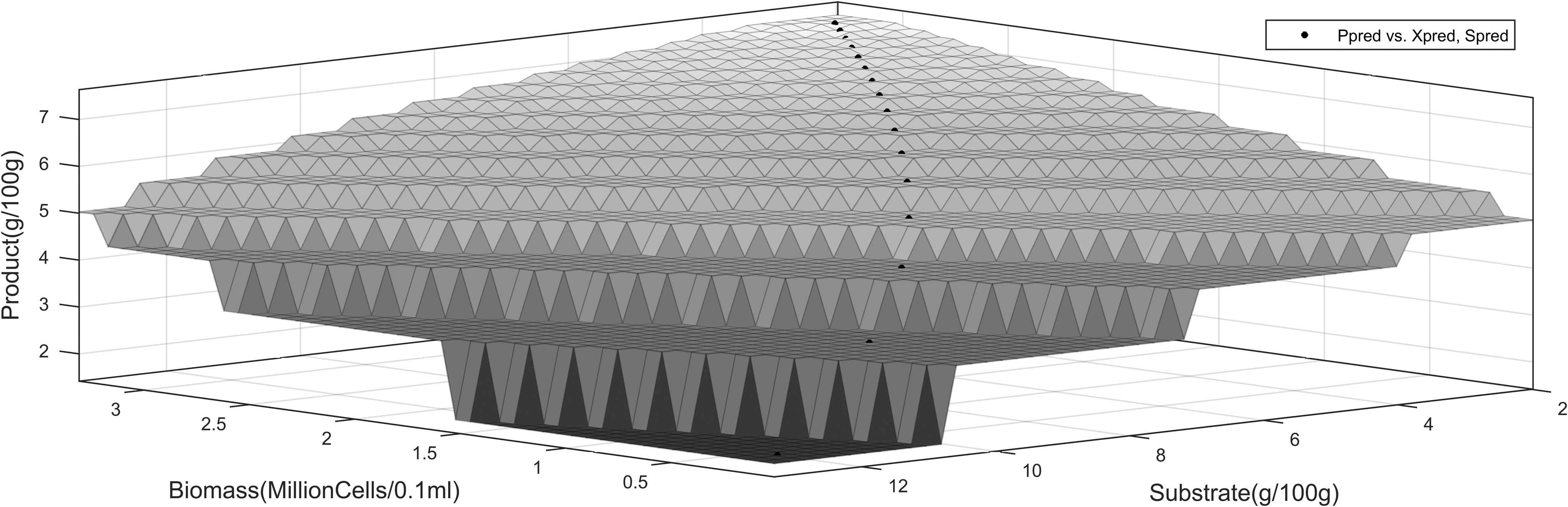
The three-dimensional profiles using the proximal interpolant method, implemented using the Matlab curve fitting tool, are shown in Figs. 5–6 ). They present the dynamics of product interpolated with substrate and time.

Results of Model Parameters and Simulations

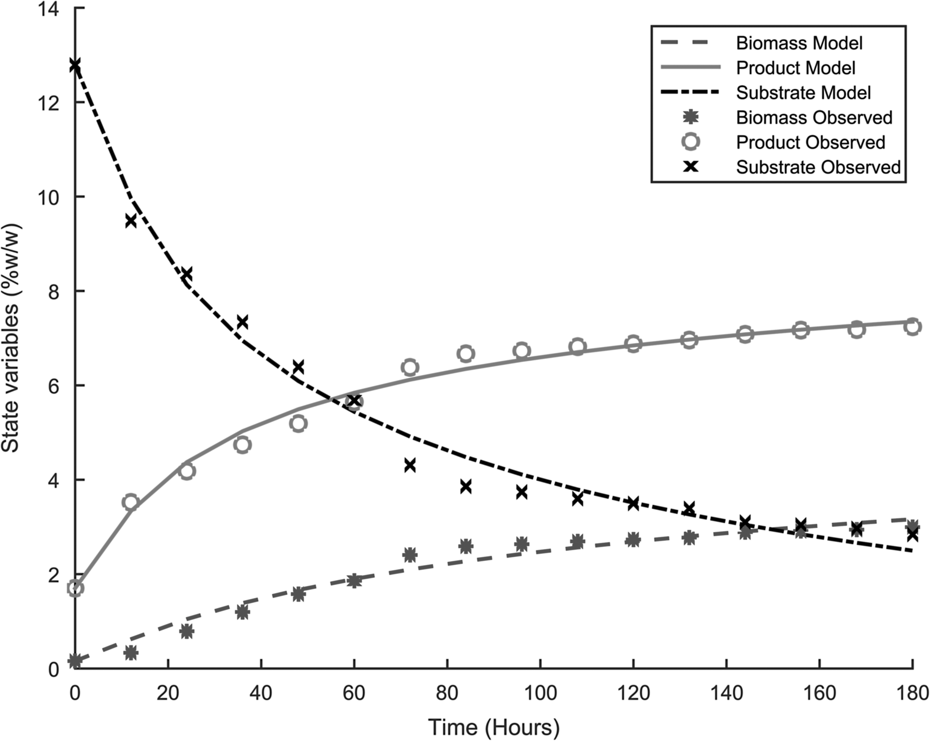
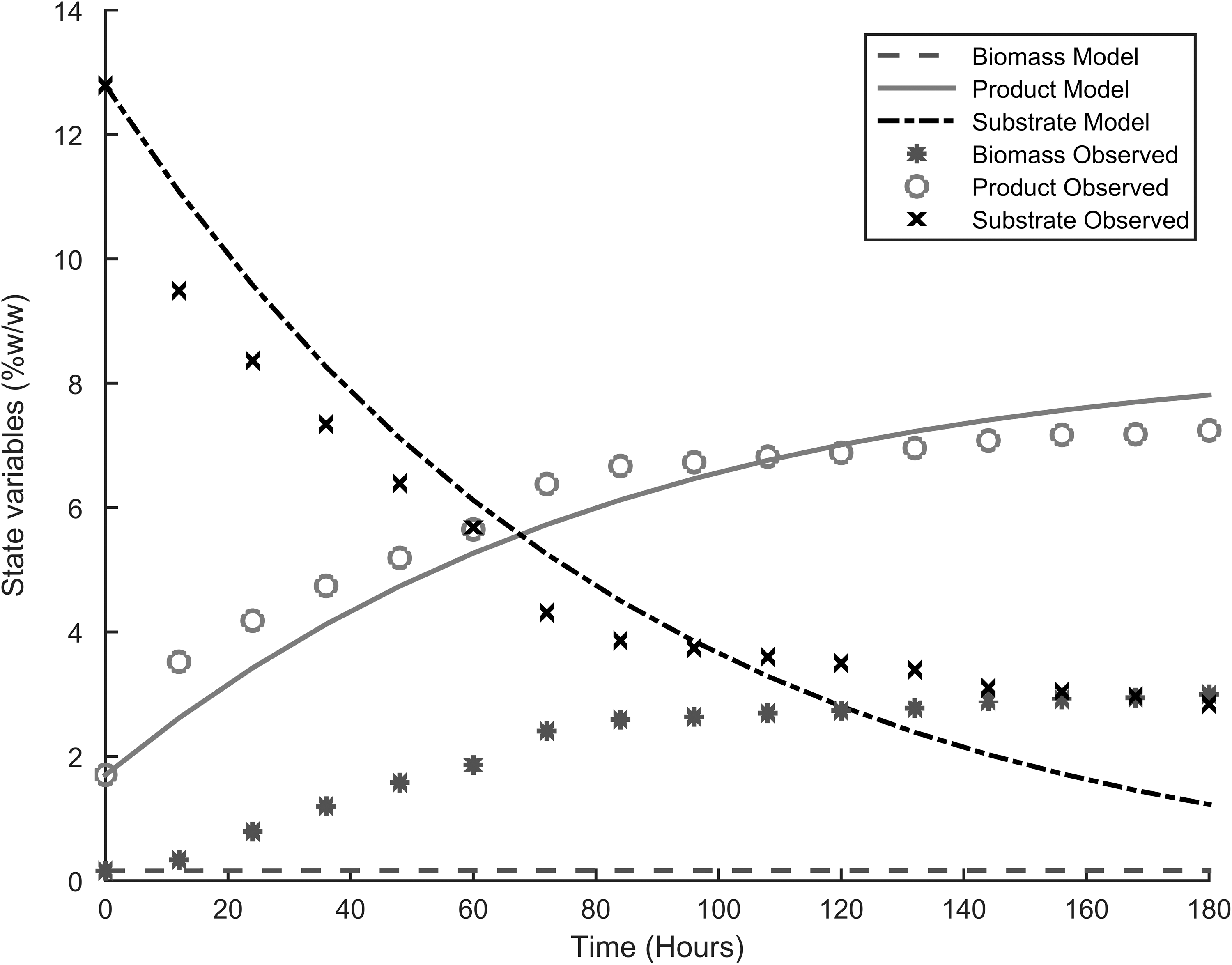
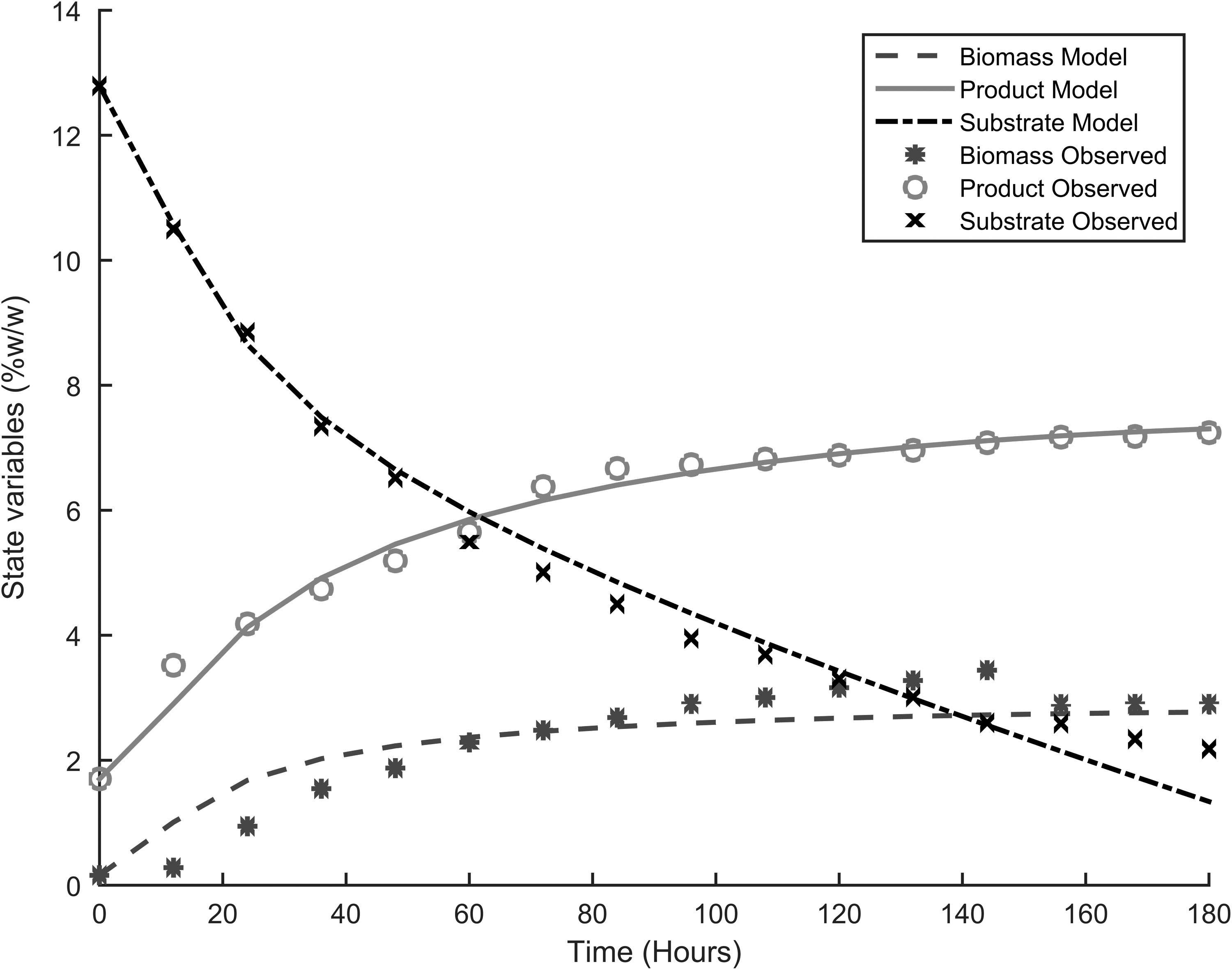
Table 3 presents the parameters for the four different models used to describe the dynamics of fermentation, and Figs. 1 –4 show the fitting of the models with respect to the experimental data. The results were unexpected. First both substrate and product inhibition exists in the alcoholic fermentation of cassava extracts, with the LS-EP and ES-EP models describing the inhibition dynamics with relatively high accuracy (having lower model errors). Second, the results confirmed our previous observations that modeling only product inhibition but did not describe with high accuracy the alcoholic fermentation of cassava extracts, suggesting the presence of substrate inhibition. The dynamics described by conventional Monod equation—in the case of no inhibition—showed a very high error, confirming the presence of inhibitions.

Fig. 1.

Experimental results and model fitting, LS-EP.

Fig. 2.

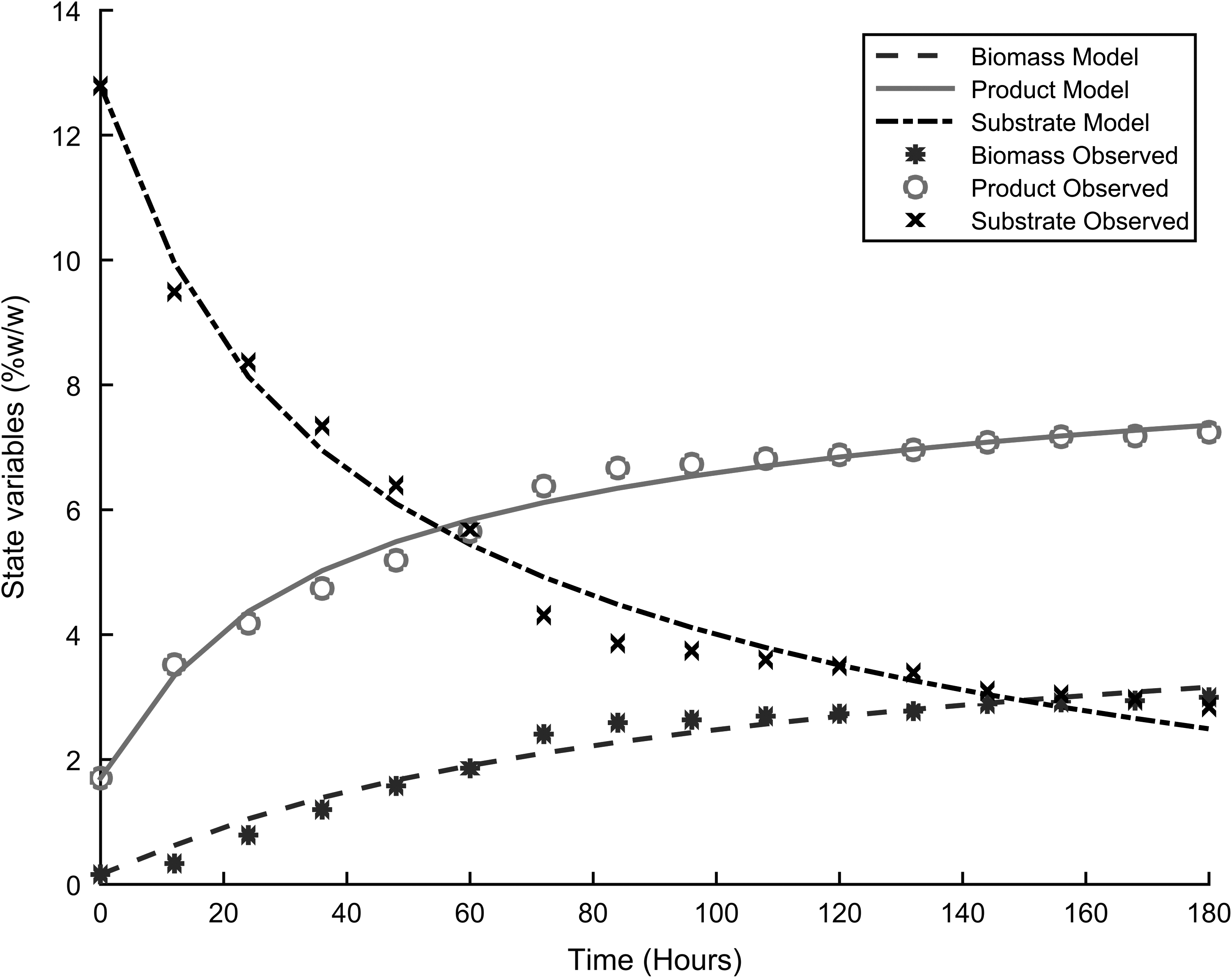
Experimental results and model fitting, LS-LP.

Fig. 3.

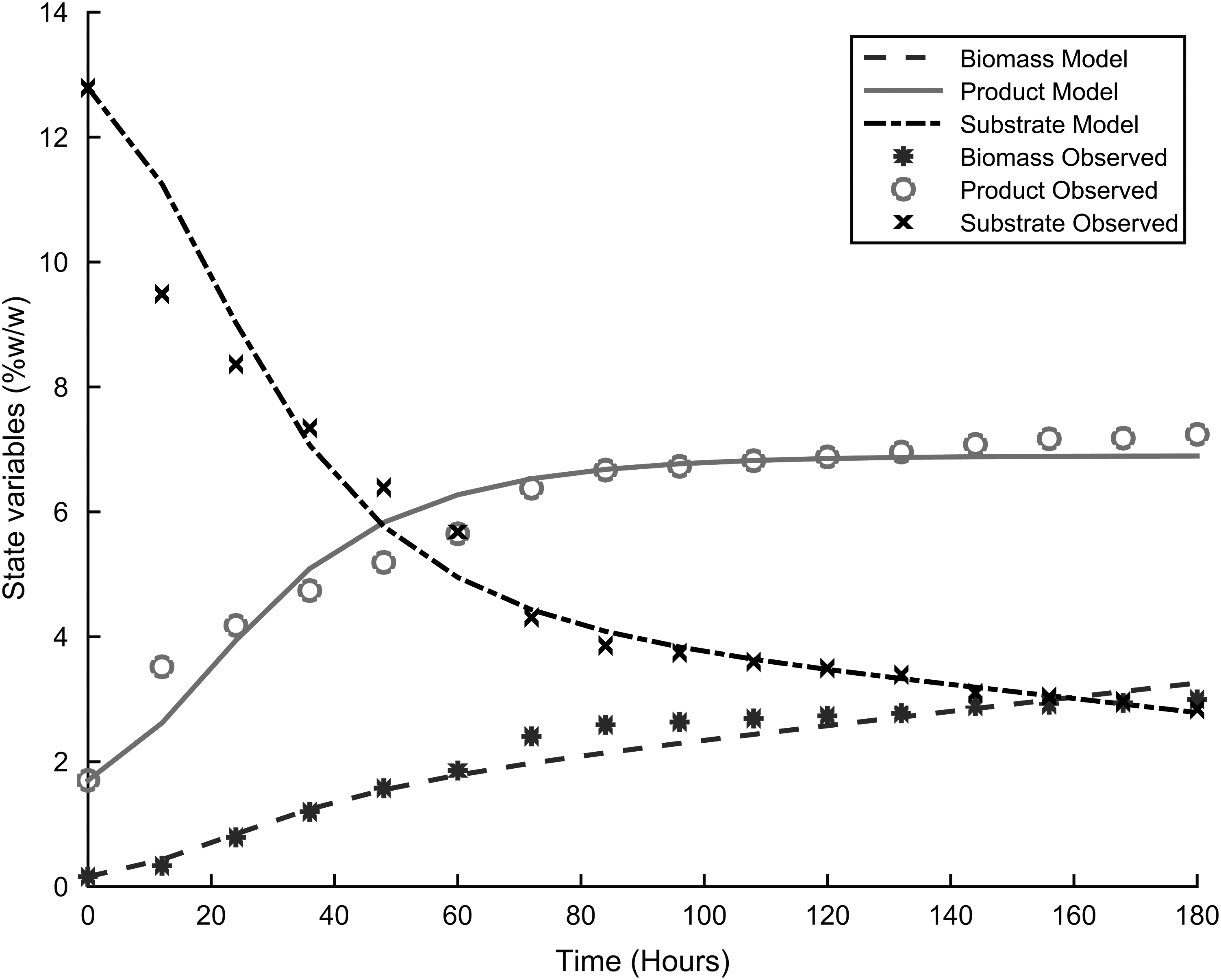
Experimental results and model fitting, ES-EP.

Fig. 4.

Experimental results and model fitting, ES-LP.

Table 3.

Model Parameters for Alcoholic Fermentation of Cassava Extract

		Inhibition
MODEL PARAMETERS	MONOD (NO INHIBITION)	LINEAR S LINEAR P	LINEAR S EXPONENTIAL P	EXPONENTIAL S LINEAR P	EXPONENTIAL S EXPONENTIAL P
\documentclass{aastex}\usepackage{amsbsy}\usepackage{amsfonts}\usepackage{amssymb}\usepackage{bm}\usepackage{mathrsfs}\usepackage{pifont}\usepackage{stmaryrd}\usepackage{textcomp}\usepackage{portland, xspace}\usepackage{amsmath, amsxtra}\pagestyle{empty}\DeclareMathSizes{10}{9}{7}{6}\begin{document}$$ { \mu_{max}}$$ \end{document}	0.0100	0.0100	3.0000	2.4342	2.9996
\documentclass{aastex}\usepackage{amsbsy}\usepackage{amsfonts}\usepackage{amssymb}\usepackage{bm}\usepackage{mathrsfs}\usepackage{pifont}\usepackage{stmaryrd}\usepackage{textcomp}\usepackage{portland, xspace}\usepackage{amsmath, amsxtra}\pagestyle{empty}\DeclareMathSizes{10}{9}{7}{6}\begin{document}$$ {q_{pmax}}$$ \end{document}	8.4851	14.5352	7.1381	7.1395	183.4561
\documentclass{aastex}\usepackage{amsbsy}\usepackage{amsfonts}\usepackage{amssymb}\usepackage{bm}\usepackage{mathrsfs}\usepackage{pifont}\usepackage{stmaryrd}\usepackage{textcomp}\usepackage{portland, xspace}\usepackage{amsmath, amsxtra}\pagestyle{empty}\DeclareMathSizes{10}{9}{7}{6}\begin{document}$$ {K_{isx}}$$ \end{document}	—	0.3131	0.0001	0.0001	0.0001
\documentclass{aastex}\usepackage{amsbsy}\usepackage{amsfonts}\usepackage{amssymb}\usepackage{bm}\usepackage{mathrsfs}\usepackage{pifont}\usepackage{stmaryrd}\usepackage{textcomp}\usepackage{portland, xspace}\usepackage{amsmath, amsxtra}\pagestyle{empty}\DeclareMathSizes{10}{9}{7}{6}\begin{document}$$ {K_{isp}}$$ \end{document}	—	0.0010	0.0021	0.0010	0.2002
\documentclass{aastex}\usepackage{amsbsy}\usepackage{amsfonts}\usepackage{amssymb}\usepackage{bm}\usepackage{mathrsfs}\usepackage{pifont}\usepackage{stmaryrd}\usepackage{textcomp}\usepackage{portland, xspace}\usepackage{amsmath, amsxtra}\pagestyle{empty}\DeclareMathSizes{10}{9}{7}{6}\begin{document}$$ {K_{ix}}$$ \end{document}	—	0.9539	0.5411	0.1264	0.5453
\documentclass{aastex}\usepackage{amsbsy}\usepackage{amsfonts}\usepackage{amssymb}\usepackage{bm}\usepackage{mathrsfs}\usepackage{pifont}\usepackage{stmaryrd}\usepackage{textcomp}\usepackage{portland, xspace}\usepackage{amsmath, amsxtra}\pagestyle{empty}\DeclareMathSizes{10}{9}{7}{6}\begin{document}$$ {K_{ip}}$$ \end{document}	—	0.1475	0.8968	0.1450	1.2437
\documentclass{aastex}\usepackage{amsbsy}\usepackage{amsfonts}\usepackage{amssymb}\usepackage{bm}\usepackage{mathrsfs}\usepackage{pifont}\usepackage{stmaryrd}\usepackage{textcomp}\usepackage{portland, xspace}\usepackage{amsmath, amsxtra}\pagestyle{empty}\DeclareMathSizes{10}{9}{7}{6}\begin{document}$$ {K_{sx}}$$ \end{document}	249.9991	1.0090	67.607	249.9969	66.2282
\documentclass{aastex}\usepackage{amsbsy}\usepackage{amsfonts}\usepackage{amssymb}\usepackage{bm}\usepackage{mathrsfs}\usepackage{pifont}\usepackage{stmaryrd}\usepackage{textcomp}\usepackage{portland, xspace}\usepackage{amsmath, amsxtra}\pagestyle{empty}\DeclareMathSizes{10}{9}{7}{6}\begin{document}$$ {K_{sp}}$$ \end{document}	199.9997	198.8989	9.5495	199.9999	11.9572
Y_x	0.1002	2.9782	3.0000	3.0000	2.9999
Y_p	0.5464	0.6497	0.6131	0.6389	0.6131
G_s	0.0010	0.0017	0.0001	0.0011	0.0001
M_s	0.0100	0.0017	0.0001	0.0011	0.0001
Model error	94.0344	7.3934	2.8012	7.5115	2.7975

Another important parameter in fermentation kinetics is the specific rate of ethanol accumulation in the medium. The parameter estimation results indicated high maximal rate of product formation—183.4561 with the ES-EP model compared to 7.1381 for LS-EP model. This suggests that even though both models showed similar accuracy in describing fermentation dynamics, designing a control policy with the ES-EP model will result in a high process productivity in terms of ethanol accumulation. It should be noted that the product inhibition had a higher effect on the fermentation process than substrate inhibition; this is apparent due to the product inhibition coefficients being very high compared to those for substrate inhibition.

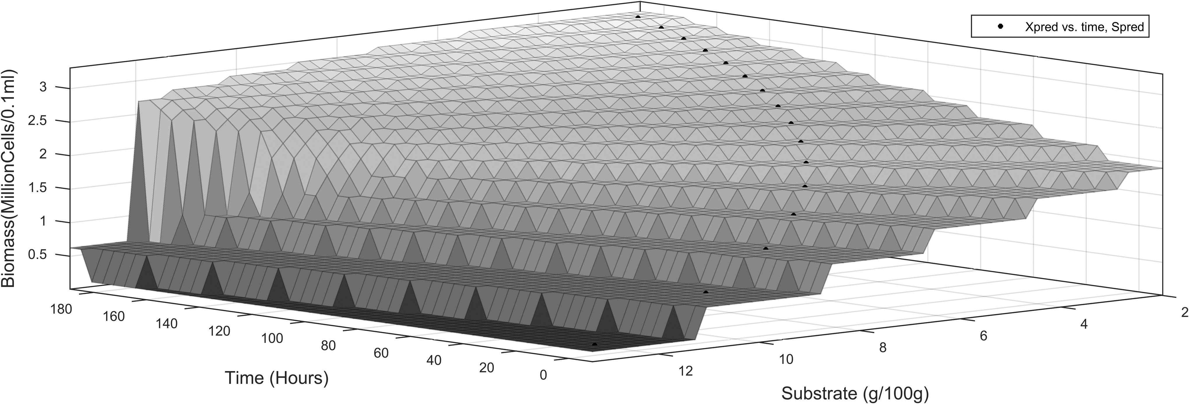
This is also explained by the fact that most of the cyanide in the cassava, which could result in substrate toxicity, is removed during upstream processing. The high product inhibition is in accordance with the work by Ingledew, which showed that substrate and product were among the environmental stresses to S. cerevisiae during alcoholic fermentation.¹⁰ Table 4 and Table 5 present the model statistical validity using two sample F-tests for variance. The results show that at a 99% confidence interval, LS-EP and the ES-EP model predictions showed no significant difference with the experimental data. In the early stages of the fermentation process, product formation occurs quickly. This decreases in intensity as substrate concentration decreases in the bioreactor. This can be attributed to the high sugar concentrations the cells encounter after the hydrolysis process. This exerts osmotic stress on the cells, resulting in transient instabilities in the reactor.^9,10,14 This stress decreases along with the sugar concentration, up to a point where the systems achieves a stable steady state and the rate of product formation becomes constant. The interpolation results for cell growth were similar (Figs. 5 –7 ).

Fig. 5.

Product dynamics versus substrate utilization and time, ES-EP inhibition model.

Fig. 6.

Dynamics of cell growth versus substrate utilization and time, ES-EP inhibition model.

Fig. 7.

Dynamics of cell growth versus substrate utilization and cell growth, ES-EP inhibition model.

Table 4.

Model Statistical Validity with Kinetics Exponential Substrate and Exponential Product Inhibition, with Two Sample F-Tests for Variance

	BIOMASS		PRODUCT		SUBSTRATE
	EXPERIMENTAL (XOBS)	MODEL (XPRED)	EXPERIMENTAL (POBS)	MODEL (PPRED)	EXPERIMENTAL (SOBS)	MODEL (SPRED)
Mean	2.093	2.113	5.881	5.886	5.275	5.280
Standard Error	0.245	0.228	0.403	0.397	0.722	0.727
Standard Deviation	0.979	0.913	1.613	1.588	2.889	2.909
Observations	16	16	16	16	16	16
Confidence Interval	0.990		0.990		0.990
f	0.8695		0.9682		1.0143
Pr(F < f) Two-tailed	0.7900		0.9509		0.9785

Table 5.

Model Statistical Validity with Kinetics Linear Substrate and Exponential Product Inhibition with Two Sample F-Tests for Variance

	BIOMASS		PRODUCT		SUBSTRATE
	EXPERIMENTAL (XOBS)	MODEL (XPRED)	EXPERIMENTAL (POBS)	MODEL (PPRED)	EXPERIMENTAL (SOBS)	MODEL (SPRED)
Mean	2.093	2.112	5.881	5.886	5.275	5.280
Standard Error	0.245	0.228	0.403	0.397	0.722	0.727
Standard Deviation	0.979	0.914	1.613	1.588	2.889	2.910
Observations	16	16	16	16	16	16
Confidence Interval	0.990		0.990		0.990
f	0.8719		0.9682		1.0144
Pr(F < f) Two-tailed	0.7941		0.9508		0.9783

Product Inhibition Results

The product inhibition and model statistical validation results are shown in Tables 6 –8 and Figures 8 –11 .

Table 6.

Model Parameters for Fermentation Using Cassava Extracts

	INHIBITION
Model Parameters	No Inhibition	Linear	SGS	Exponential
\documentclass{aastex}\usepackage{amsbsy}\usepackage{amsfonts}\usepackage{amssymb}\usepackage{bm}\usepackage{mathrsfs}\usepackage{pifont}\usepackage{stmaryrd}\usepackage{textcomp}\usepackage{portland, xspace}\usepackage{amsmath, amsxtra}\pagestyle{empty}\DeclareMathSizes{10}{9}{7}{6}\begin{document}$$ { \mu _{max}}$$ \end{document}	0.0100	0.3326	2.9996	4.9991
\documentclass{aastex}\usepackage{amsbsy}\usepackage{amsfonts}\usepackage{amssymb}\usepackage{bm}\usepackage{mathrsfs}\usepackage{pifont}\usepackage{stmaryrd}\usepackage{textcomp}\usepackage{portland, xspace}\usepackage{amsmath, amsxtra}\pagestyle{empty}\DeclareMathSizes{10}{9}{7}{6}\begin{document}$$ {q_{pmax}}$$ \end{document}	8.4851	51.3560	5.8755	2.6067
\documentclass{aastex}\usepackage{amsbsy}\usepackage{amsfonts}\usepackage{amssymb}\usepackage{bm}\usepackage{mathrsfs}\usepackage{pifont}\usepackage{stmaryrd}\usepackage{textcomp}\usepackage{portland, xspace}\usepackage{amsmath, amsxtra}\pagestyle{empty}\DeclareMathSizes{10}{9}{7}{6}\begin{document}$$ {P_{xmax}}$$ \end{document}	—	—	6.8884	—
\documentclass{aastex}\usepackage{amsbsy}\usepackage{amsfonts}\usepackage{amssymb}\usepackage{bm}\usepackage{mathrsfs}\usepackage{pifont}\usepackage{stmaryrd}\usepackage{textcomp}\usepackage{portland, xspace}\usepackage{amsmath, amsxtra}\pagestyle{empty}\DeclareMathSizes{10}{9}{7}{6}\begin{document}$$ {P_{pmax}}$$ \end{document}	—	—	6.7637	—
\documentclass{aastex}\usepackage{amsbsy}\usepackage{amsfonts}\usepackage{amssymb}\usepackage{bm}\usepackage{mathrsfs}\usepackage{pifont}\usepackage{stmaryrd}\usepackage{textcomp}\usepackage{portland, xspace}\usepackage{amsmath, amsxtra}\pagestyle{empty}\DeclareMathSizes{10}{9}{7}{6}\begin{document}$$ {K_{ix}}$$ \end{document}	—	0.1466	—	0.8290
\documentclass{aastex}\usepackage{amsbsy}\usepackage{amsfonts}\usepackage{amssymb}\usepackage{bm}\usepackage{mathrsfs}\usepackage{pifont}\usepackage{stmaryrd}\usepackage{textcomp}\usepackage{portland, xspace}\usepackage{amsmath, amsxtra}\pagestyle{empty}\DeclareMathSizes{10}{9}{7}{6}\begin{document}$$ {K_{ip}}$$ \end{document}	—	0.1013	—	0.6347
\documentclass{aastex}\usepackage{amsbsy}\usepackage{amsfonts}\usepackage{amssymb}\usepackage{bm}\usepackage{mathrsfs}\usepackage{pifont}\usepackage{stmaryrd}\usepackage{textcomp}\usepackage{portland, xspace}\usepackage{amsmath, amsxtra}\pagestyle{empty}\DeclareMathSizes{10}{9}{7}{6}\begin{document}$$ {K_{sx}}$$ \end{document}	249.9991	13.5297	231.0673	52.4603
\documentclass{aastex}\usepackage{amsbsy}\usepackage{amsfonts}\usepackage{amssymb}\usepackage{bm}\usepackage{mathrsfs}\usepackage{pifont}\usepackage{stmaryrd}\usepackage{textcomp}\usepackage{portland, xspace}\usepackage{amsmath, amsxtra}\pagestyle{empty}\DeclareMathSizes{10}{9}{7}{6}\begin{document}$$ {K_{sp}}$$ \end{document}	199.9997	249.9655	199.9957	25.2593
Y_x	0.1002	19.9983	1.0000	0.4297
Y_p	0.5464	0.7589	1.1878	6.9998
G_s	0.0010	0.0010	0.0010	0.0010
M_s	0.0100	0.0100	0.0100	0.0100
Model error	94.0344	4.8107	7.8655	5.5755

Table 7.

Model Statistical Validity with Kinetics Linear Substrate and Linear Product Inhibitions, Two Sample F-test for Variance

	BIOMASS		PRODUCT		SUBSTRATE
	EXPERIMENTAL (XOBS)	MODEL (XPRED)	EXPERIMENTAL (POBS)	MODEL (PPRED)	EXPERIMENTAL (SOBS)	MODEL (SPRED)
Mean	2.296	2.255	5.881	5.855	5.291	5.299
Standard error	0.261	0.183	0.403	0.416	0.788	0.816
Standard deviation	1.044	0.733	1.613	1.666	3.151	3.266
Observations	16	16	16	16	16	16
Confidence interval	0.990		0.990		0.990
F	0.4934		1.0665		1.0742
Pr(F < f) two-tailed	0.1832		0.9024		0.8915

Table 8.

Model Statistical Validity with Kinetics Exponential Substrate and Linear Product Inhibitions, Two Sample F-Test for Variance

	BIOMASS		PRODUCT		SUBSTRATE
	EXPERIMENTAL (XOBS)	MODEL (XPRED)	EXPERIMENTAL (POBS)	MODEL (PPRED)	EXPERIMENTAL (SOBS)	MODEL (SPRED)
Mean	2.296	2.180	5.880	5.910	5.291	5.308
Standard error	0.261	0.227	0.403	0.375	0.788	0.826
Standard deviation	1.044	0.909	1.613	1.501	3.151	3.306
Observations	16	16	16	16	16	16
Confidence interval	0.990		0.990		0.990
F	0.7572		0.8654		1.1005
Pr(F < f) two-tailed	0.5969		0.7831		0.853

Fig. 8.

Experimental results and model fitting, no inhibition (Monod-Model).

Fig. 9.

Experimental results and model fitting, linear inhibition model.

Fig. 10.

Experimental results and model fitting, Sudden growth stop inhibition model.

Fig. 11.

Experimental results and model fitting, exponential inhibition model.

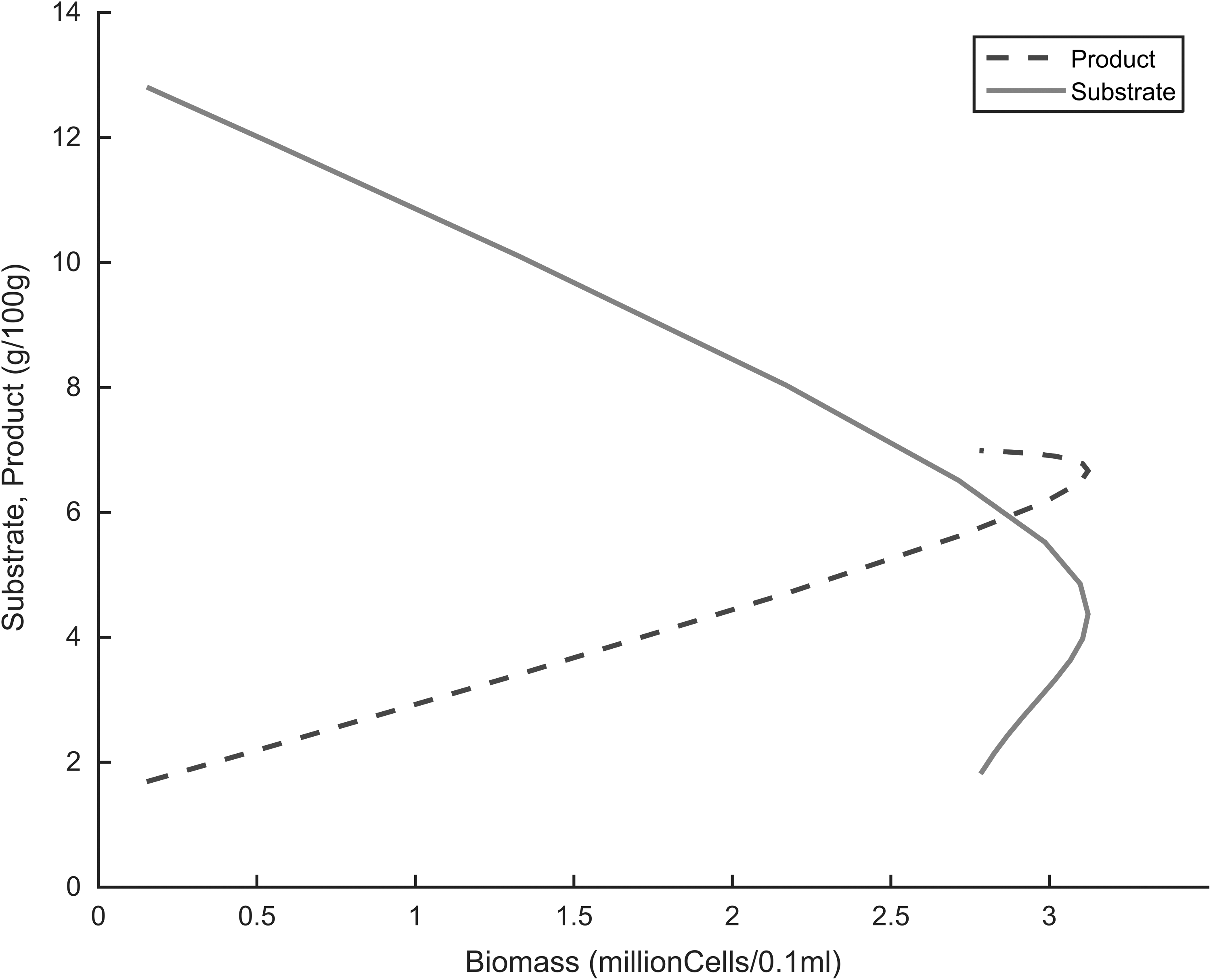
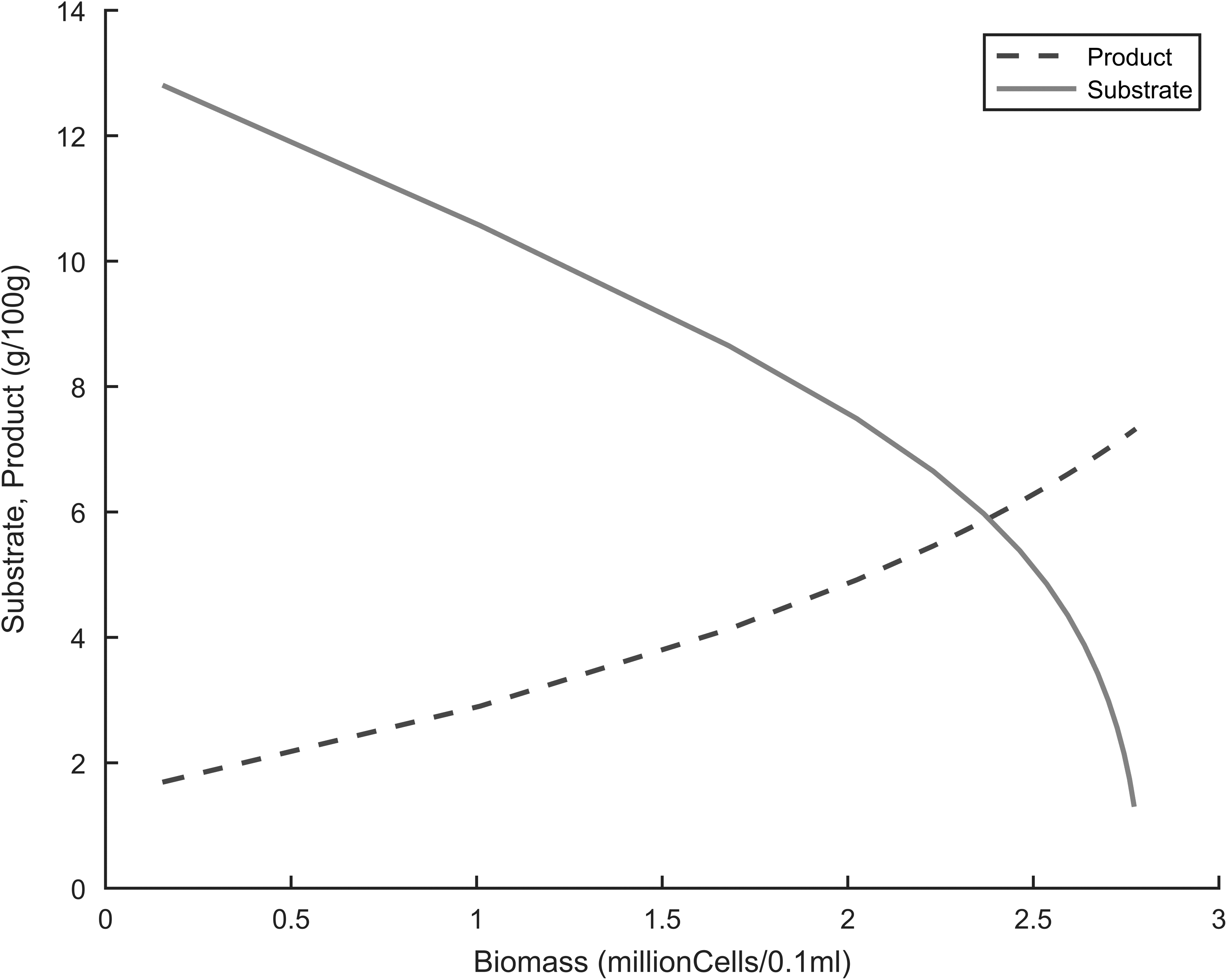
Understanding how the substrate and product vary in the fermenter as the cells grow is also important in a fermentation process. The linear and exponential inhibition models were both used to simulate these variations. Figures 12 and 13 showed a decrease in substrate concentration and an increase in product concentration with cell growth. However, with the linear model, a curve-like behavior was observed at the edges of the plot, being more intense with the product profile. There are two theories explain this behavior: ethanol inhibition or stationary/decline phases in batch growth kinetics. In the case of ethanol inhibition, the linear model has a relatively high maximal rate of product formation, and ethanol rapidly accumulates to inhibitory levels, leading to disruption of the cell membranes and thus nonlinearity in the substrate-consumption and product-formation profiles.^5

–9,14 Regarding the stationary or decline theory in batch growth kinetics, the curve-like behavior observed in the linear model can be attributed to the fact that cells get to the stationary and decline phases. At these stages the cells no longer consume substrate to produce ethanol as in the exponential phase, hence the observed nonlinearity.

Fig. 12.

Simulation of substrate and product as a function of biomass during fermentation, linear inhibition kinetics.

Fig. 13.

Simulation of substrate and product as a function of biomass during fermentation using exponential inhibition kinetics.

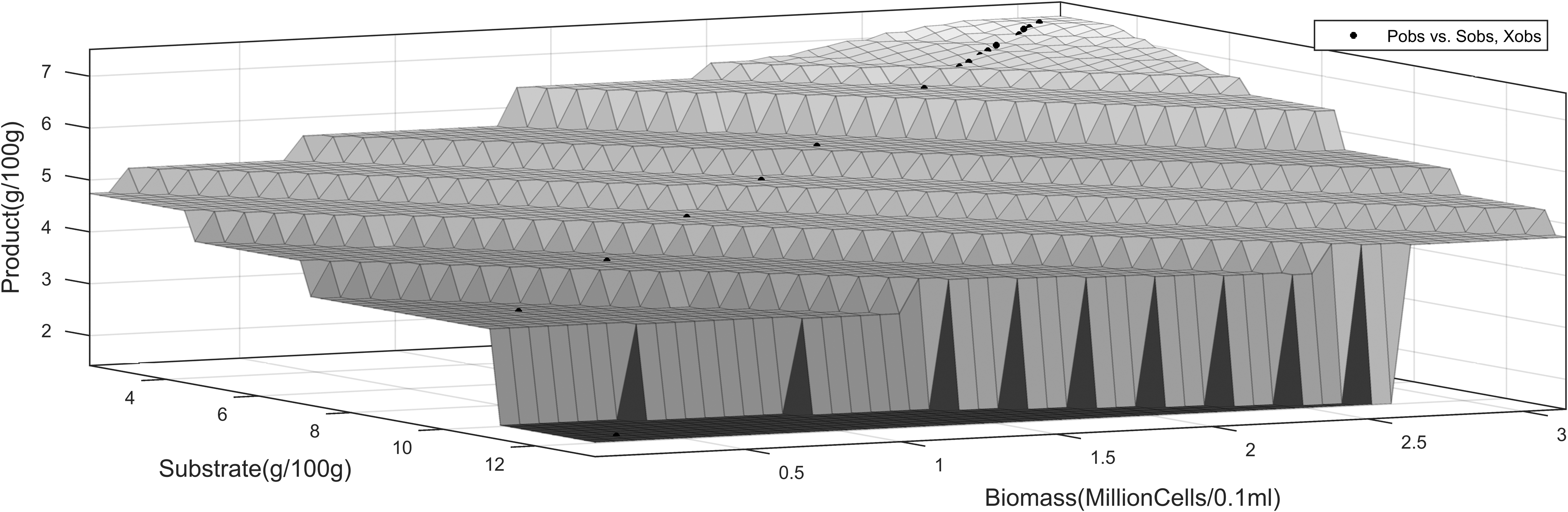
The smallest discrepancy between the model and experimental data was for the linear model, which was somewhat unsatisfactory compared to previous studies modeling ethanol fermentation. This high model error could be attributed to the existence of substrate inhibition that was not considered in the modeling. Cassava contains intrinsic microbial inhibitors such as linamarin, which is converted to hydrocyanic acid during the upstream processes.⁴ Figure 14 presents product formation with cell growth and substrate consumption and further confirms this assertion. Nonlinearities are observed at high substrate concentration, which gradually decrease in intensity as substrate concentration decreases.

Fig. 14.

Dynamics of product formation with cell growth and substrate consumption.

Conclusions

A mathematical approach to study the substrate product inhibitor on the kinetics of alcoholic fermentation has been presented. The results show that there exist both product and substrate inhibition in the alcoholic fermentation of cassava extracts, with product inhibition having a higher effect. The kinetics of the fermentation process was determined using at a 99% confidence interval using two mathematical models. There are differences with respect to process productivity with the ES-EP model showing to result in a higher ethanol yield if used to design a control policy. 3D simulations showed that there exist transient instabilities at the start of fermentation process attributed to high sugar concentrations encountered immediately after hydrolysis which exert osmotic stress on yeast cells resulting in transient instabilities in the bioreactor.

The modeling of product inhibition in the alcoholic fermentation of cassava extracts has been presented. The results show that ethanol inhibition can be described with a 99% confidence interval as being either a linear or exponential inhibitory impact on ethanol concentration. The linear model resulted in a very high maximal rate of ethanol accumulation, hence rapidly approaching inhibitory levels. We recommend developed models should be used to determined optimal controls that minimize the effects of such inhibitions. We also recommend substrate inhibition to be modeled on the kinetics of cell growth and product formation in an attempt to further decrease the discrepancy between model and experimental data.

The obtained models described with high accuracy with 99% confidence interval. It is also recommended that an optimal control problem using the developed models should be set up and solved to determine the fermentation conditions that minimize the effect of such inhibitions during the fermentation of cassava extracts.

Footnotes

Acknowledgments

Our team expresses sincere thanks to the Intra-ACP under the project Strengthening African Higher Education through Academic Mobility (STREAM). We are also thankful to Breweries Ghana for supplying us with industrial data to validate our model.

Author Disclosure Statement

No competing financial interests exist.

References

Olivier

. Mass balance modelling of bioprocesses. (2001) Available at: www.sop.inria.fr/comore/ICTP_Modelling_Bernard.pdf (Last accessed August 2016 ).

Tonukari

. Cassava and the future of starch. African J Biotechnol, 2004; 7(1).

Alford

. Bioprocess control: Advances and challenges. Computers Chem Eng, 2006; 30:1464–1475.

Philbrick

, Hill

, Alexander

. Physiological and biochemical changes associated with linamarin and administration to rats. Toxicol Asql Pharmacol, 1977; 42:539.

Chen

, McDonald

. Oscillatory behavior of Saccharomyces cerevisiae in continuous culture: I. Effects of pH and nitrogen levels. Biotechnol Bioeng, 1990; 36:19–27.

Chen

, McDonald

. Oscillatory behavior of Saccharomyces cerevisiae in continuous culture: II. Analysis of cell synchronization and metabolism. Biotechnol Bioeng, 1990; 36:28–38.

Beuse

MRB

, Kopmann

AHD

, Thoma

. Effect of dilution rate on the mode of oscillation in continuous culture of Saccharomyces cerevisiae . J Biotechnol, 1998; 61:15–31.

Beuse

MRB

, Komann

AHD

, Thoma

. Oxygen, pH value, and carbon source induced changes of the mode of oscillations in Saccharomyces cerevisiae . Biotechnol Bioeng, 1999; 63:410–417.

Fengwu

. 2007. Process oscillations in continuous ethanol fermentation with Saccharomyces cerevisiae . (Doctoral thesis). Ontario, Canada: University of Waterloo.

10.

Russell

. Similarities and differences in the responses of microorganisms to biocides. J Antimicrob Chemother, 2003; 52:750–763.

11.

Hinshelwood

. The chemical kinetics of the bacterial cell. London, UK: Clarendon Press Oxford, 1946.

12.

Ghose

, Tyagi

. Rapid ethanol fermentation of cellulose hydrolysate. II. Product and substrate inhibition and optimization of fermentor design. Biotechnol Bioeng, 1979; 21:1401–1420.

13.

Aiba

, Shoda

, Nagatani

. Kinetics of product inhibition in alcohol fermentation. Biotechnol Bioeng, 1968; 10:845–864.

14.

Sutton

. (2011) A Novozymes short report: Fermentation inhibitors. Available at: http://bioenergy.novozymes.com/Documents/Ferm_SR_Inhibitors.pdf (Last accessed August 2016 ).