A Multiscale Computational Approach to Estimating Axonal Damage under Inertial Loading of the Head

Abstract

A computational modeling framework is developed to estimate the location and degree of diffuse axonal injury (DAI) under inertial loading of the head. DAI is one of the most common pathological features of traumatic brain injury and is characterized by damage to the neural axons in the white matter regions of the brain. We incorporate the microstructure of the white matter (i.e., the fiber orientations and fiber dispersion) through the use of diffusion tensor imaging (DTI), and model the white matter with an anisotropic, hyper-viscoelastic constitutive model. The extent of DAI is estimated using an axonal strain injury criterion. A novel injury analysis method is developed to quantify the degree of axonal damage in the fiber tracts of the brain and identify the tracts that are at the greatest risk for functional failure. Our modeling framework is applied to analyze DAI in a real-life ice hockey incident that resulted in concussive injury. To simulate the impact, two-dimensional finite element (FE) models of the head were constructed from detailed MRI and DTI data and validated using available human head experimental data. Acceleration loading curves from accident reconstruction data were then applied to the FE models. The rotational (rather than translational) accelerations were shown to dominate the injury response, which is consistent with previous studies. Through this accident reconstruction, we demonstrate a conceptual framework to estimate the degree of axonal injury in the fiber tracts of the human brain, enabling the future development of relationships between computational simulation and neurocognitive impairment.

Introduction

T raumatic brain injury (TBI) is a debilitating injury that is caused by an external mechanical stimulus to the head. TBIs are most commonly sustained through falls, vehicular accidents, and assaults; however, TBIs resulting from collisions in sports-related incidents and from exposure to blasts in theater have received a great deal of attention within the past few years. One of the most common pathological features of TBI is diffuse axonal injury (DAI), also called traumatic axonal injury (TAI). This type of injury is characterized by damage to the neural axons in the white matter of the brain and is caused by sudden inertial loads to the head.¹ As this injury occurs at the cellular level, the structural signature of this injury is not visible with conventional medical imaging modalities, which makes DAI difficult to diagnose. The inability to visualize the injury in vivo also makes the progression of axonal injury difficult to study. Computational models that can capture the location and degree of axonal injury as a result of specific stimuli and correlate this to predicted cognitive deficits would be of great benefit.

Finite element (FE) models are useful tools for understanding the development of DAI in TBI incidents. Significant improvements have been made in finite element models of brain trauma over the years.^2
–4 Early FE models of the head included little anatomical detail. The brain tissue was often treated as a homogenous, isotropic material, and internal structures, such as the falx cerebri and ventricles, were not included. In recent years, the structural detail in computational head models has been greatly enhanced through the use of medical imaging data. Both magnetic resonance imaging (MRI) and computed tomography (CT) scans have been utilized to segment anatomical structures such as the gray matter, white matter, ventricles, cerebrospinal fluid (CSF), falx cerebri, tentorium cerebelli, dura, arachnoid, and pia mater. The material models used for brain tissue have also improved from simple linear elastic constitutive models to models that include some of the intrinsic nonlinearities, strain rate dependence, and anisotropy of brain tissue.^5
–7 However, constructing three-dimensional (3-D) FE head models that contain both a high level of anatomical detail and sophisticated constitutive models remains a challenge. There is often a tradeoff between the sophistication of the model and the computational cost of running an analysis.

In addition to the accurate representation of the geometry and material behavior, a critical element in a computational model of TBI is the definition of injury. Although numerous injury criteria have been proposed for TBI, the appropriate measure of injury to use in a computational analysis remains a subject of debate. Is brain injury a stress-driven process or a strain-driven process? What are the thresholds for injury? Traditionally, the injury criteria for TBI have been acceleration based.⁸ These macroscale measures of injury are easily measured in experimental studies and therefore, have become a basis for numerous brain injury protocols, including vehicle safety standards and helmet design standards. However, macroscale measures of injury cannot generally be related to specific microscale injury modalities. In contrast, tissue level thresholds for injury are difficult to determine experimentally, and, therefore, are commonly determined through an FE analysis. A real-life trauma event is simulated using an FE model, and the results from the analysis are correlated with clinical data from the subject, such as observations of concussion and/or TBI pathologies. One limitation of this approach is that the determined injury criteria are highly dependent on the fidelity of the FE model used in the analysis. As a result, the injury thresholds developed from one FE model may not be suitable to apply to another FE model that uses a significantly different material stiffness for the brain tissue. Therefore, independent validation of material behavior and injury thresholds is important in computational approaches to TBI.

As an alternative to the conventional approaches of determining injury criteria for TBI, injury criteria can also be defined based on the cellular mechanisms of injury.⁷ In vitro and in vivo models of TBI offer a platform for quantifying mechanical thresholds for axonal injury directly. These models have been used to study the effects of cellular strain and strain rate on the injury response of neural cells.^9,10 Although these experimental platforms provide a way to directly measure the thresholds for axonal injury, the injury thresholds determined from these studies are not widely used in FE head models. One reason for this has been the difficulty in coupling the cellular and tissue length scales in an FE model.

In recent work, we have developed a formal multiscale procedure for coupling the cellular mechanisms of axonal injury to the deformation of brain tissue.⁷ We modeled the white matter with an anisotropic, hyperelastic constitutive model and incorporated the structural orientation of the neural axons through the use of diffusion tensor imaging (DTI). An axonal strain injury (ASI) criterion was used as a measure of DAI. This injury criterion is based on the stretch injury response of neural axons, and the thresholds for injury were derived directly from in vivo experiments. In this work, we extend this multiscale modeling framework to a two-dimensional (2-D) full head FE model. The constitutive model for the brain tissue is extended to include fiber dispersion and viscoelasticity, and a novel method is developed to quantify the degree of axonal damage in the neural tracts through the use of a white matter atlas. The multiscale modeling framework is applied to estimate the degree of axonal damage in a real-life ice hockey incident that resulted in concussive injury. Our injury analysis method provides a novel way to relate the likely damage in the brain to the cognitive deficits that can develop from TBI, for specific incidents.

This article is organized as follows. The Methods section describes the anisotropic constitutive model for white matter, the ASI criterion that we use to define injury in our FE model, and the use of DTI to incorporate the microstructure of the white matter. The development and validation of our 2-D FE head models are also presented in the Methods section. In the Results section, our computational approach is applied to analyze DAI in a real-life head impact incident using accident reconstruction data, and we derive new insights into the effects of the components of acceleration, the degree of anisotropy, and the ASI criterion on the injury response.

Methods

Viable computational models of TBI must be able to accurately represent the behavior of tissues under loading, and they must be able to accurately predict injury. To better represent the mechanical behavior of brain tissue, we used a constitutive model for the white matter that accounted for its anisotropic behavior, and to better predict DAI, we used an injury criterion that was based on the cellular mechanisms of axonal injury: the ASI criterion. Both the constitutive model and injury criterion were dependent upon the local orientation of the neural axons, and we used an in vivo imaging technique called DTI to define these fiber orientations (Fig. 1). The following sections describe the constitutive model for brain tissue, the ASI criterion, and the application of DTI. This is followed by a description of the FE modeling framework.

FIG. 1.

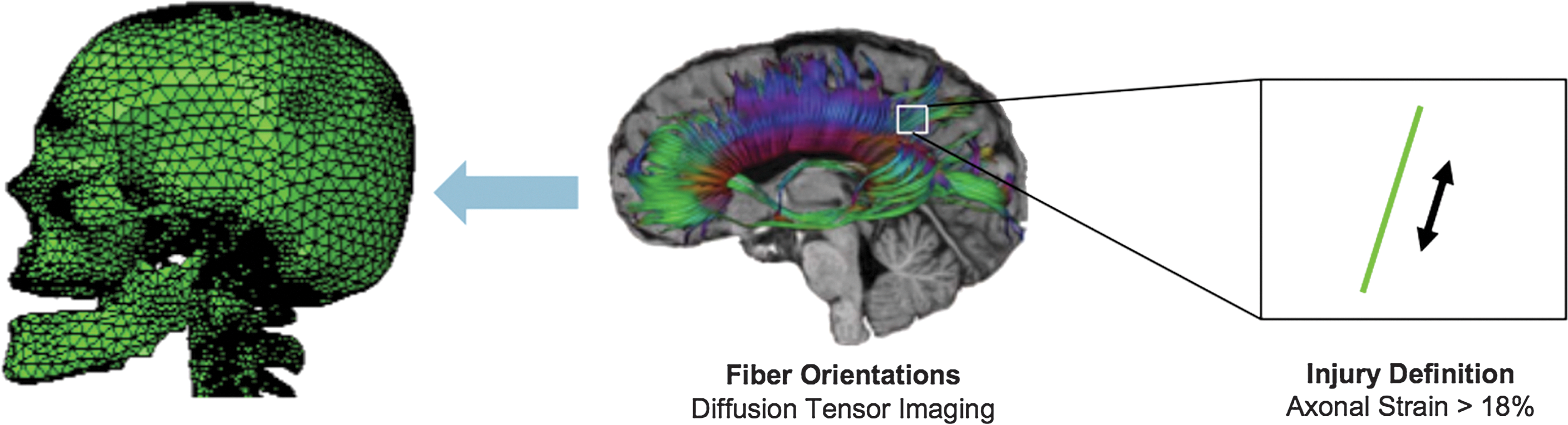
Diffuse axonal injury is measured through an oriented strain measure: the axonal strain. The axonal strain is defined as the strain component resolved in the direction of fiber alignment (right image). The primary direction of fiber alignment within each elemental region of our model is obtained directly through diffusion tensor imaging. (Left image courtesy of Dr. Reuben Kraft; center image adapted from shockmd.com). Color image is available online at www.liebertonline.com/neu

Constitutive model for brain tissue

The white matter in the brain primarily consists of an organized arrangement of neural axons and is generally considered anisotropic.¹¹ In contrast, the gray matter primarily contains the cell bodies of neurons, and is considered to be an isotropic material. In our previous work, we used an anisotropic, hyperelastic constitutive model to model the white matter.⁷ Here, we extend our constitutive model to include both viscoelasticity and fiber dispersion. We model the white matter using the Holzapfel–Gasser–Ogden (HGO) strain energy function derived by Gasser et al.¹²; several other studies have also applied this strain energy function to represent the anisotropic response of white matter.^13
–15 The HGO strain energy function is defined as: \documentclass{aastex}\usepackage{amsbsy}\usepackage{amsfonts}\usepackage{amssymb}\usepackage{bm}\usepackage{mathrsfs}\usepackage{pifont}\usepackage{stmaryrd}\usepackage{textcomp}\usepackage{portland, xspace}\usepackage{amsmath, amsxtra}\pagestyle{empty}\DeclareMathSizes{10}{9}{7}{6}\begin{document} \begin{align*}W = \frac {\mu} {2} (\bar {I} _1 - 3) + \frac {k_1} {2k_2} \mathop\sum_ {\alpha = 1} ^N \left\{e^ {k_2 \langle \bar {E} \alpha \rangle^ {2}} - 1 \right\} + \frac {K} {2} \left(\frac {J^2 - 1} {2} - \ln J \right) \tag {1} \end{align*} \end{document}

With \documentclass{aastex}\usepackage{amsbsy}\usepackage{amsfonts}\usepackage{amssymb}\usepackage{bm}\usepackage{mathrsfs}\usepackage{pifont}\usepackage{stmaryrd}\usepackage{textcomp}\usepackage{portland, xspace}\usepackage{amsmath, amsxtra}\pagestyle{empty}\DeclareMathSizes{10}{9}{7}{6}\begin{document} \begin{align*}\bar{E}_{\alpha} = \kappa (\bar{I}_1 - 3) + (1 - 3 \kappa) (\bar{I}_{4 \alpha} - 1) \tag{2}\end{align*} \end{document}

where μ is the shear modulus of the isotropic matrix, k₁ accounts for the additional stiffness provided by the fibers, k₂ is a dimensionless material parameter that controls the nonlinearity of the anisotropic response, N is the total number of fiber families (α=1,…,N), K is the effective bulk modulus of the material, and J is the volume change ratio. The modified invariant, \documentclass{aastex}\usepackage{amsbsy}\usepackage{amsfonts}\usepackage{amssymb}\usepackage{bm}\usepackage{mathrsfs}\usepackage{pifont}\usepackage{stmaryrd}\usepackage{textcomp}\usepackage{portland, xspace}\usepackage{amsmath, amsxtra}\pagestyle{empty}\DeclareMathSizes{10}{9}{7}{6}\begin{document} $$\bar {I}_1$$ \end{document} , is defined as \documentclass{aastex}\usepackage{amsbsy}\usepackage{amsfonts}\usepackage{amssymb}\usepackage{bm}\usepackage{mathrsfs}\usepackage{pifont}\usepackage{stmaryrd}\usepackage{textcomp}\usepackage{portland, xspace}\usepackage{amsmath, amsxtra}\pagestyle{empty}\DeclareMathSizes{10}{9}{7}{6}\begin{document} \begin{align*}\bar{I}_1 = tr \overline{{\bf C}} \tag{3}\end{align*} \end{document}

and the modified pseudo-invariant, \documentclass{aastex}\usepackage{amsbsy}\usepackage{amsfonts}\usepackage{amssymb}\usepackage{bm}\usepackage{mathrsfs}\usepackage{pifont}\usepackage{stmaryrd}\usepackage{textcomp}\usepackage{portland, xspace}\usepackage{amsmath, amsxtra}\pagestyle{empty}\DeclareMathSizes{10}{9}{7}{6}\begin{document} $$\bar {I}_4$$ \end{document} , is defined as \documentclass{aastex}\usepackage{amsbsy}\usepackage{amsfonts}\usepackage{amssymb}\usepackage{bm}\usepackage{mathrsfs}\usepackage{pifont}\usepackage{stmaryrd}\usepackage{textcomp}\usepackage{portland, xspace}\usepackage{amsmath, amsxtra}\pagestyle{empty}\DeclareMathSizes{10}{9}{7}{6}\begin{document} \begin{align*}\bar{I}_4 = {\bf A \cdot \overline {C} A} \tag{4}\end{align*} \end{document}

where \documentclass{aastex}\usepackage{amsbsy}\usepackage{amsfonts}\usepackage{amssymb}\usepackage{bm}\usepackage{mathrsfs}\usepackage{pifont}\usepackage{stmaryrd}\usepackage{textcomp}\usepackage{portland, xspace}\usepackage{amsmath, amsxtra}\pagestyle{empty}\DeclareMathSizes{10}{9}{7}{6}\begin{document} $$\overline {\rm C}$$ \end{document} is the deviatoric component of the right Cauchy–Green deformation tensor and A is a unit vector representing the fiber direction in the reference configuration. The \documentclass{aastex}\usepackage{amsbsy}\usepackage{amsfonts}\usepackage{amssymb}\usepackage{bm}\usepackage{mathrsfs}\usepackage{pifont}\usepackage{stmaryrd}\usepackage{textcomp}\usepackage{portland, xspace}\usepackage{amsmath, amsxtra}\pagestyle{empty}\DeclareMathSizes{10}{9}{7}{6}\begin{document} $$\bar{I}_4$$ \end{document} pseudo-invariant is directly related to the stretch, λ, of the fibers in the material \documentclass{aastex}\usepackage{amsbsy}\usepackage{amsfonts}\usepackage{amssymb}\usepackage{bm}\usepackage{mathrsfs}\usepackage{pifont}\usepackage{stmaryrd}\usepackage{textcomp}\usepackage{portland, xspace}\usepackage{amsmath, amsxtra}\pagestyle{empty}\DeclareMathSizes{10}{9}{7}{6}\begin{document} $$(\bar{I}_4 = \lambda^2)$$ \end{document} .¹⁶

In the case of brain tissue, we assume that the fiber component of the material consists of the neural axons and its cytoskeletal components. The fiber dispersion of the neural axons is represented through the structure parameter κ in Equation 2. Assuming that the fibers are distributed according to a π-periodic von Mises distribution, the lower limit of κ becomes 0, which represents regions with perfectly aligned fibers (i.e., transverse isotropy), and the upper limit becomes 1/3, which describes regions with randomly oriented fibers (i.e., isotropy).¹² In the HGO model, it is assumed that the fibers cannot support a compressive load. This assumption is enforced through the Macauley bracket \documentclass{aastex}\usepackage{amsbsy}\usepackage{amsfonts}\usepackage{amssymb}\usepackage{bm}\usepackage{mathrsfs}\usepackage{pifont}\usepackage{stmaryrd}\usepackage{textcomp}\usepackage{portland, xspace}\usepackage{amsmath, amsxtra}\pagestyle{empty}\DeclareMathSizes{10}{9}{7}{6}\begin{document} $$\langle \bullet \rangle$$ \end{document} , which is defined as \documentclass{aastex}\usepackage{amsbsy}\usepackage{amsfonts}\usepackage{amssymb}\usepackage{bm}\usepackage{mathrsfs}\usepackage{pifont}\usepackage{stmaryrd}\usepackage{textcomp}\usepackage{portland, xspace}\usepackage{amsmath, amsxtra}\pagestyle{empty}\DeclareMathSizes{10}{9}{7}{6}\begin{document} $$\langle x \rangle = \frac {1} {2} (\mid x \mid + x)$$ \end{document} and ensures that the anisotropic part of the response appears only if the fibers are in tension.

We made a few simplifications to the model to reduce the number of material parameters. First, it was assumed that only a single family of fibers existed in the material; therefore, N was set equal to 1. Second, the contribution of k₂ to the material response was assumed to be minimal (k₂→0). From these simplifications, the total strain energy potential became \documentclass{aastex}\usepackage{amsbsy}\usepackage{amsfonts}\usepackage{amssymb}\usepackage{bm}\usepackage{mathrsfs}\usepackage{pifont}\usepackage{stmaryrd}\usepackage{textcomp}\usepackage{portland, xspace}\usepackage{amsmath, amsxtra}\pagestyle{empty}\DeclareMathSizes{10}{9}{7}{6}\begin{document} \begin{align*}W = \frac {\mu} {2} (\bar {I} _1 - 3) + \frac {k_1} {2} \langle \bar {E_1} \rangle^2 + \frac {K} {2} \left(\frac {J^2 - 1} {2} - \ln J \right) \tag {5} \end{align*} \end{document}

We should note that if κ=0 and k₂→0, the HGO model reduces to the quadratic reinforcing model that we used in our previous work.⁷

The HGO strain energy function was applied to model both the white matter and gray matter. As the gray matter was isotropic, the κ parameter was set equal to 1/3 for the gray matter regions. For the white matter regions, κ was determined directly from the diffusion tensor imaging data, which will be described in the following section. The rest of the material parameters in the HGO model (μ, k₁, k₂, and K) remained the same for both the white and gray matter.

We incorporated the time-dependent behavior of brain tissue into our model using a quasilinear viscoelastic approach. It was assumed that only the deviatoric behavior contributed to the viscoelastic response of the material and that only the isotropic shear modulus was a function of time. We approximated the isotropic shear relaxation modulus using a first order Prony series \documentclass{aastex}\usepackage{amsbsy}\usepackage{amsfonts}\usepackage{amssymb}\usepackage{bm}\usepackage{mathrsfs}\usepackage{pifont}\usepackage{stmaryrd}\usepackage{textcomp}\usepackage{portland, xspace}\usepackage{amsmath, amsxtra}\pagestyle{empty}\DeclareMathSizes{10}{9}{7}{6}\begin{document} \begin{align*}\mu (t) = \mu_ \infty + (\mu_0 - \mu_ \infty) e^{- \beta t} \tag{6}\end{align*} \end{document}

where μ₀ is the instantaneous shear modulus, μ_∞ is the long-term shear modulus at equilibrium, and β is the decay constant.

ASI Criterion

An ASI criterion⁷ is used to estimate the degree of diffuse axonal injury in our FE model. The threshold for injury is derived from an experimental study by Bain and Meaney,¹⁷ who stretched the optic nerve of a guinea pig in vivo at strain rates of 30–60/sec and analyzed the resulting functional and morphological damage caused by stretch. Bain and Meaney measured the degree of axonal damage by recording changes in the electrical potentials generated by the neural cells and by staining for common markers of the axonal pathology. Strain thresholds were defined based on the onset of functional and structural damage. Although the magnitude of cellular strain is not identically equal to the tissue-level strain measured by Bain and Meaney, because of the undulated nature of the neural axons, these strain measures are proportional to one another,¹⁸ and the tissue-level strain threshold is representative of the axonal damage that occurs at the cellular level because of stretch. Furthermore, as these experiments were conducted in vivo, the tissue was not completely isolated from the systemic environment, and, therefore, the determined strain thresholds were a physiologically relevant measure of injury. An “optimal” strain threshold (which optimized both the specificity and sensitivity measures) of 18% was determined for the onset of electrophysiological impairment by Bain and Meaney, and an optimal threshold of 21% was determined for morphological damage. As functional damage can occur without the presence of structural damage, we adapt the lower tissue-level threshold of 18% as the axonal strain injury tolerance threshold in our study.

Incorporation of neural tract alignment through DTI

The primary direction of fiber alignment, A, and the degree of fiber dispersion, κ, must be defined to describe the material response of the white matter using the HGO model and to apply the ASI criterion. These parameters vary spatially throughout the brain and can be defined through the use of DTI. DTI is an MRI technique that provides an in vivo method for determining the orientation of neural axons within the human brain. DTI works by measuring the diffusion of water molecules along different orientations in the brain. It is based on the concept that water molecules diffuse faster in the direction parallel to neural axons than perpendicular to them;¹⁹ therefore, the direction with the greatest diffusion correlates with the primary direction of fiber alignment. Each voxel of the DTI image contains 3-D information about the diffusion as represented by a “diffusion tensor.”²⁰ A fiber orientation map can be constructed from the eigenvectors of the diffusion tensor. The eigenvector corresponding to the largest eigenvalue represents the primary direction of fiber alignment for a given voxel. Other useful scalar quantities can also be derived from the diffusion tensor. For example, the fractional anisotropy (FA) is a normalized measure of the degree of diffusion anisotropy, and it is computed as follows: \documentclass{aastex}\usepackage{amsbsy}\usepackage{amsfonts}\usepackage{amssymb}\usepackage{bm}\usepackage{mathrsfs}\usepackage{pifont}\usepackage{stmaryrd}\usepackage{textcomp}\usepackage{portland, xspace}\usepackage{amsmath, amsxtra}\pagestyle{empty}\DeclareMathSizes{10}{9}{7}{6}\begin{document} \begin{align*}FA = \sqrt {\frac {1} {2}} \frac {\sqrt {(\lambda_1 - \lambda_2) ^2 + (\lambda_1 - \lambda_3) ^2 + (\lambda_2 - \lambda_3) ^2}} {\sqrt {\lambda_1^2 + \lambda_2^2 + \lambda_3^2}} \tag {7} \end{align*} \end{document}

where λ_i represent the eigenvalues of the diffusion tensor.²¹ The fractional anisotropy ranges from a value of 0 (which indicates that the diffusion is uniform in all directions) to a value of 1 (which indicates that the diffusion is along a single direction).²² Therefore, a high FA value correlates with regions that have a large degree of fiber alignment, and a low FA value correlates with regions that are isotropic.

The fiber orientation map and FA map from DTI provides the primary direction of fiber alignment and the degree of fiber dispersion, respectively. Although the local fiber orientations can be directly obtained from the fiber orientation map, the fiber dispersion values determined from the FA map are not equal to the fiber dispersion parameter (κ) used in the HGO model. Therefore, a relationship must be developed between κ and FA to define the fiber dispersion in the material model. The FA is computed from the eigenvalues of the diffusion tensor, and the diffusion tensor represents the distribution of fiber orientations within a voxel. In the HGO model, the distribution of fiber orientations is represented through a generalized structure tensor H. For a transversely isotropic representation, the structure tensor is reduced to the following form¹²: \documentclass{aastex}\usepackage{amsbsy}\usepackage{amsfonts}\usepackage{amssymb}\usepackage{bm}\usepackage{mathrsfs}\usepackage{pifont}\usepackage{stmaryrd}\usepackage{textcomp}\usepackage{portland, xspace}\usepackage{amsmath, amsxtra}\pagestyle{empty}\DeclareMathSizes{10}{9}{7}{6}\begin{document} \begin{align*}{\bf H} = \kappa {\bf I} + (1 - 3 \kappa) {\bf A} \otimes {\bf A} \tag{8}\end{align*} \end{document}

where I is the identity tensor, and A is the unit vector denoting the primary fiber direction in the reference configuration. For any given unit vector A representing the fiber direction, the eigenvalues of the structure tensor can be defined as: \documentclass{aastex}\usepackage{amsbsy}\usepackage{amsfonts}\usepackage{amssymb}\usepackage{bm}\usepackage{mathrsfs}\usepackage{pifont}\usepackage{stmaryrd}\usepackage{textcomp}\usepackage{portland, xspace}\usepackage{amsmath, amsxtra}\pagestyle{empty}\DeclareMathSizes{10}{9}{7}{6}\begin{document} \begin{align*}\lambda_1 = 1 - 2 \kappa , \quad \lambda_2 = \kappa , \quad \lambda_3 = \kappa \tag{9}\end{align*} \end{document}

These eigenvalues are functions of the fiber dispersion parameter, κ. To develop a relationship between FA and κ, these eigenvalues are substituted into Equation 7, and the equation is solved for κ: \documentclass{aastex}\usepackage{amsbsy}\usepackage{amsfonts}\usepackage{amssymb}\usepackage{bm}\usepackage{mathrsfs}\usepackage{pifont}\usepackage{stmaryrd}\usepackage{textcomp}\usepackage{portland, xspace}\usepackage{amsmath, amsxtra}\pagestyle{empty}\DeclareMathSizes{10}{9}{7}{6}\begin{document} \begin{align*}\kappa = \frac {1} {2} \frac {- 6 + 4 {\rm FA} ^2 + 2 \sqrt {3 {\rm FA} ^2 - 2 {\rm FA} ^4}} {- 9 + 6 FA^2} \tag {10} \end{align*} \end{document}

This equation is used to compute a corresponding κ value for each FA value in the FA map. The derivation is based on the assumption that the diffusion tensor from the DTI and the structure tensor from the HGO model are both representative of the distribution of fiber orientations, and the eigenvalues of the diffusion tensor scale with the eigenvalues of the structure tensor.

2-D FE modeling approach for the head

The constitutive model for brain tissue and the fiber data from the DTI are implemented into 2-D FE head models. The models are created from T1-weighted MRI and DTI from a single normal subject (female, age 68, Caucasian). The nominal resolution of the imaging matrix is ∼1 mm for the MRI and 2 mm for the DTI. As the diffusion tensor images are obtained in a different reference coordinate system than that of the MRI, the data sets are co-registered so that both sets are described in the same coordinate system. As a result of the co-registration process, there is a one-to-one spatial correspondence between the two data sets; therefore, the voxel locations in the DTI maps can easily be mapped to the element locations in the FE mesh. The structures of the head are segmented using the MRI data and discretized to create the FE mesh. The DTI data are then used to define the local fiber orientation and fiber dispersion in the white matter.

Because of the computational expense of simulating inertial loading problems in 3-D, we chose to idealize the 3-D geometry through multiple 2-D FE models of the head. By modeling the problem in 2-D, we are able to incorporate a higher level of anatomical detail and use increasingly sophisticated constitutive models for the brain tissue, while keeping the computational cost low. As the geometry of the structures within the head varies significantly along different anatomical planes, we constructed our 2-D finite element models along the three primary anatomical planes: the coronal plane, the axial plane, and the sagittal plane (Fig. 2). A single FE model was constructed along each anatomical plane. These particular planes are chosen because they are representative of the different structural geometries found in the head. Furthermore, the acceleration curves derived from accident reconstructions in the literature are often decomposed into components along these anatomical orientations. By constructing our models along these planes, the loading conditions from accident reconstruction data could be applied to our FE models in a direct fashion.

FIG. 2.

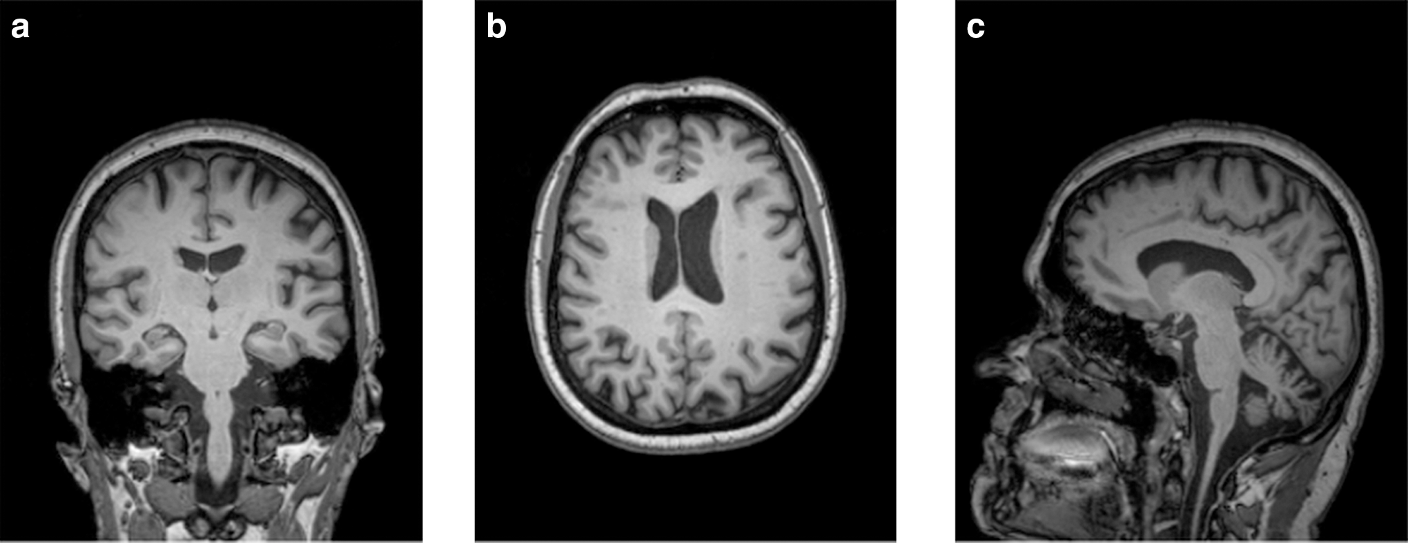
Magnetic resonance images (T1-MRI) of the three sections chosen for the FE analysis. These sections are along (a) the coronal plane, (b) the axial plane, and (c) the sagittal plane.

Segmentation and mesh generation

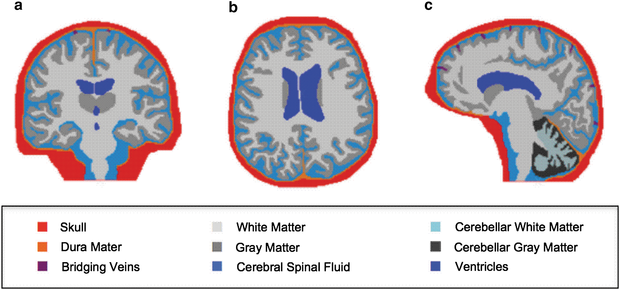
To construct the FE mesh, the structures of the head were first defined and manually segmented from the MRIs using ITK-Snap 2.0.0 software (www.itksnap.org).²³ The segmented structures are shown in Figure 3 and include the skull, the dura mater (including both the falx cerebri and the tentorium cerebelli), the bridging veins, the cerebral white and gray matter, the cerebellar white and gray matter, the CSF, and the ventricles. The spatial resolution of the segmented structures was limited by the image resolution of the MRI, which is 1 mm.

FIG. 3.

The segmented structures are shown for (a) the coronal slice model, (b) the axial slice model, and (c) the sagittal slice model. Color image is available online at www.liebertonline.com/neu

The 2-D FE meshes were generated from the segmented images using OOF2 2.0.5 software developed by the United States National Institute of Standards and Technology (www.ctcms.nist.gov/oof). A mesh convergence study was conducted to determine the appropriate mesh density. As a result of the mesh density study, the following meshes were generated for each model plane: 11,409 elements (coronal mesh), 13,177 elements (axial mesh), and 12,438 elements (sagittal mesh). The element sizes in each FE model ranged from 1 to 2 mm, which is comparable to the resolution of the imaging data. No mesh smoothing was performed during the mesh generation process.

Incorporation of DTI data

Using the co-registered fiber orientation and FA maps, the fiber orientations and fiber dispersions were assigned to each element of the FE mesh based on the spatial location within the DTI maps. As the FE models are in two-dimensions, the 3-D orientation vectors had to be projected onto the 2-D plane of the models. The fiber dispersions were computed from the FA maps using Equation 10. For elements that overlapped several voxels of the DTI data, a weighted average of the orientation vectors and dispersion values was taken to give a single vector and dispersion value for each element. The incorporated fiber orientations are shown in Figure 4 for the axial FE model.

FIG. 4.

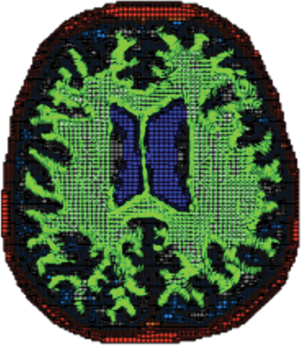
The fiber orientations obtained from diffusion tensor imaging are shown in green on the finite element mesh of the axial model. Color image is available online at www.liebertonline.com/neu

Material properties

The white matter and gray matter were modeled using the HGO model as described earlier. Three potential sets of material parameters were derived for the brain tissue (Table 1), and one set was chosen based on our validation results. That validated parameter set was then used to represent the brain tissue in our accident reconstruction study.

Table 1.

Brain Tissue Material Properties

Material	ρ (kg/m³)	K (GPa)	μ₀ (Pa)	μ_∞ (Pa)	k₁ _∞ (Pa)	k₂	κ	β (s⁻¹)
High modulus
White matter	1040	2.19	34,000	6400	2716	0.0001	from DTI	700
Gray matter	1040	2.19	34,000	6400	2716	0.0001	1/3	700
Mid modulus
White matter	1040	2.19	17,000	3200	1354	0.0001	from DTI	700
Gray matter	1040	2.19	17,000	3200	1354	0.0001	1/3	700
Low modulus
White matter	1040	2.19	1520	286	121	0.0001	from DTI	700
Gray matter	1040	2.19	1520	286	121	0.0001	1/3	700

DTI, diffusion tensor imaging.

The first set of parameters, which we refer to as “low modulus parameters,” were derived by fitting the HGO model to tensile tests on white matter tissue samples performed by Velardi et al.²⁴ As the fiber dispersion in the tested specimens was unknown, it was assumed that the fibers were perfectly aligned with minimal dispersion (κ=0). The fitting procedure is described in more detail in Wright and Ramesh.⁷ The fit to the Velardi data provided the shear modulus and the fiber reinforcement parameter as μ=286 Pa and k₁ =121 Pa, respectively. The second set of parameters (“high modulus parameters”) were derived by adjusting the moduli from the Velardi fit to be consistent with moduli values widely used in computational simulations,^25

–29 but with the ratio of the fiber reinforcement parameter to the shear modulus (k₁ /μ) kept the same as the Velardi fit. The final set of parameters (“mid modulus parameters”) was chosen such that the shear modulus was 50% lower than that of the high modulus parameters.

The viscoelastic parameters for the brain tissue were determined as follows. It was assumed that the material parameters determined from the Velardi study were representative of the long-term behavior, as the tensile tests were conducted at a relatively low strain rate. A long-term to short-term shear modulus ratio of 0.19 from Zhang et al.²⁹ was used to define the instantaneous shear modulus in Equation 6, and a decay constant of 700/sc was adapted from Taylor and Ford²⁸ to define the relaxation rate.

The material properties for the remaining structures of the finite element model (skull, dura, cerebellum, bridging veins, and CSF) are listed in Tables 2 –4. The interfaces between the materials in the model were tied such that no tangential sliding or normal separation could occur. The skull and dura mater were modeled as linear elastic materials with the material properties consistent with those commonly used in computational head models.^25,30,31 Both the white and gray matter of the cerebellum were modeled through a Neo-Hookean hyperelastic strain energy function extended to include quasilinear viscoelasticity. The shear modulus of the cerebellum (Table 3) was chosen to be 24% softer than the isotropic shear modulus of the cerebral white and gray matter based on the experimental findings of Zhang et al.³² The time dependent behavior of the cerebellum was assumed to be similar to that of the cerebral white and gray matter. The bridging veins were modeled with a first-order Ogden strain-energy function. The material properties were determined by fitting the hyperelastic constitutive model to experimental stretch data from a study by Monson et al.³³ Finally, the hydrostatic behavior of the CSF and ventricles was modeled using a Mie–Gruneisen equation of state, and the deviatoric behavior was modeled by defining a shear viscosity. The material properties for the CSF (Table 4) were chosen to be similar to that of water.^34,35

Table 2.

Material Properties for the Skull, Dura Mater, and Bridging Veins

Material	ρ (kg/m³)	K (GPa)	μ₁ (kPa)	α₁	E (MPa)	ν	Strain energy function (W)
Skull	2070	—	—	—	8000	0.22	—
Dura	1133	—	—	—	31.5	0.45	—
Bridging veins	1040	2.19	25.63	11.12	—	—	\documentclass{aastex}\usepackage{amsbsy}\usepackage{amsfonts}\usepackage{amssymb}\usepackage{bm}\usepackage{mathrsfs}\usepackage{pifont}\usepackage{stmaryrd}\usepackage{textcomp}\usepackage{portland, xspace}\usepackage{amsmath, amsxtra}\pagestyle{empty}\DeclareMathSizes{10}{9}{7}{6}\begin{document} $$W = \frac {2 \mu_1} {\alpha_1} \left(\bar {\lambda} _1^ {\alpha_1} + \bar {\lambda} _2^ {\alpha_1} + \bar {\lambda} _3^ {\alpha_1} - 3 \right) + \frac {K} {2} (J - 1) ^2$$ \end{document}

Table 3.

Material Properties for the Cerebellum

Material	ρ (kg/m³)	K (GPa)	μ₀ (kPa)	μ_∞ (Pa)	β (s⁻¹)	Strain energy function (W)
Cerebellum	1040	2.19	28,845	4864	700	\documentclass{aastex}\usepackage{amsbsy}\usepackage{amsfonts}\usepackage{amssymb}\usepackage{bm}\usepackage{mathrsfs}\usepackage{pifont}\usepackage{stmaryrd}\usepackage{textcomp}\usepackage{portland, xspace}\usepackage{amsmath, amsxtra}\pagestyle{empty}\DeclareMathSizes{10}{9}{7}{6}\begin{document} $$W = \frac {\mu} {2} (\bar {I} _1 - 3) + \frac {K} {2} (J - 1) ^2 , \mu (t) = \mu_ \infty + (\mu_0 - \mu_ \infty) e^ {- \beta t}$$ \end{document}

Table 4.

Material Properties for the Cerebral Spinal Fluid (CSF)

Material	ρ₀ (kg/m³)	c₀ (m/s)	s	Γ₀	η (Pa s)	Equation of state
CSF	1004	1489	1.79	1.65	0.001	\documentclass{aastex}\usepackage{amsbsy}\usepackage{amsfonts}\usepackage{amssymb}\usepackage{bm}\usepackage{mathrsfs}\usepackage{pifont}\usepackage{stmaryrd}\usepackage{textcomp}\usepackage{portland, xspace}\usepackage{amsmath, amsxtra}\pagestyle{empty}\DeclareMathSizes{10}{9}{7}{6}\begin{document} $$p = \frac {\rho_0 c_0^2 \xi} {(1 - s \xi) ^2} \left(1 - \frac {\Gamma_0 \xi} {2} \right) + \Gamma_0 \rho_0 E_m , \xi \equiv 1 - \frac {\rho_0} {\nu}$$ \end{document}

Boundary conditions

The finite element simulations were conducted using an explicit time integration scheme in the Abaqus 6.10-EF1 commercial software package (Dassault Systémes Simulia Corp., Providence, RI). Because of the highly constrained nature of the brain tissue in the skull, a plane strain condition was assumed for the 2-D FE models. The elements used in the model were either three-node linear elements or reduced integration four-node bilinear elements. As the full neck was not modeled, a rigid base was added to the sagittal and coronal models to prevent excessive deformations from occurring at the base of the brainstem. The skull was assumed to be rigid in all the simulations. The motion of the skull was defined at a reference node placed at the center of mass (COM) of the head, and the inertial loading conditions were defined at the head COM.

Approach to injury analysis

DAI was estimated in the computational simulations using the ASI criterion. The axonal strain was defined as the nominal strain component resolved in the primary direction of fiber alignment of each element. An axonal strain threshold of 18% was chosen to indicate the onset of functional neural damage based on the experimental results of Bain and Meaney.¹⁷ The damage was assumed to be cumulative and monotonic in our simulations. Once a region exceeded the injury threshold, the region could not become undamaged during the course of the simulation.

A white matter atlas was then used to quantify the degree of axonal damage in the fiber tracts of the brain. The white matter atlas was created from T1-weighted, T2-weighted, fluid-attenuated inversion-recovery (FLAIR), and DTI images from a single, 32-year-old female subject as described in Zhang et al.³⁶ In the atlas, 130 different brain tissue structures are segmented. The segmented structures include regions within the deep white matter and the superficial white matter as well as the deep gray matter, midbrain, and brainstem. A table listing these structures can be found in the Appendix. The atlas was co-registered to our model, and the white matter regions were labeled based on the defined structures of the atlas. The segmented atlas structures are shown in Figure 5 for the three anatomical planes analyzed in our study. The percent of fiber tract damage was computed for each tract based on the total area of the tract in the model and the total damaged area of the tract as computed with the ASI criterion. Using this injury analysis method, the fiber tracts with the highest degree of damage could be determined. This information is valuable in determining the potential cognitive deficits that may result, as each fiber tract in the brain serves a role in the acquisition and processing of information.

FIG. 5.

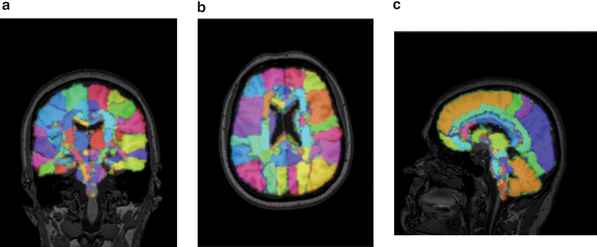
The segmented regions obtained from the white matter atlas are shown for (a) the coronal slice, (b) the axial slice, and (c) the sagittal slice. Color image is available online at www.liebertonline.com/neu

Validation of the computational model

The objective of our validation study was to verify that the appropriate material parameters and constitutive models were used in the FE models. Two experimental studies were simulated. In the first simulation, the pressure measurements from a cadaver impact experiment by Nahum et al.³⁷ were used to validate the hydrostatic behavior of the materials in our model. In the second simulation, the deviatoric behavior of the brain tissue was validated against the measured in vivo brain deformation in an inertial loading study by Sabet et al.³⁸

In the experiment by Nahum et al.,³⁷ the frontal bone of the skull of a cadaver was impacted by a rigid mass traveling at a constant velocity, and the intracranial pressure history was measured at five locations in the head: frontal region, parietal region, occipital region (both hemispheres), and posterior fossa. We simulated the experiment using our axial and sagittal 2-D FE models, as these models contained the axis of loading, and we compared the pressure results from our 2-D FE analyses to that measured experimentally. The pressure results for the posterior fossa are shown in Figure 6a, where the solid curve represents the sagittal FE results and the dashed curve represents the experimental results. Overall, the finite element models were shown to capture the hydrostatic response reasonably well. The validation study was conducted for the three sets of material parameters listed in Table 1, and the smallest difference between the experimental and simulation results was found using the “high modulus” parameters. The temporal behavior and magnitude of the pressures agreed relatively well between the simulations and experiments for most of the regions studied; however, it should be noted that the pressure magnitude in the occipital region varied by almost an order of magnitude between the experiment and the axial model simulation (see online supplementary material at http://www.liebertonline.com/neu for further details).

FIG. 6.

(a) To simulate Nahum's impact experiment, a pressure input was applied to our sagittal and axial finite element (FE) models (only sagittal model shown here). The experimentally measured pressure history (dashed, red curve) in the posterior fossa was plotted against the computed pressure history (solid, blue curve) using the “high modulus” parameters for brain tissue. (b) To simulate the Sabet's head rotation experiment, an angular rotation was applied to our axial FE model about the center of mass. The area fraction of the brain tissue exceeding a radial-circumferential shear strain of 0.04 was plotted against time. The results are shown for three sets of brain tissue parameters (high, mid, and low) and for two different experimental subjects (S1 and S2). Color image is available online at www.liebertonline.com/neu

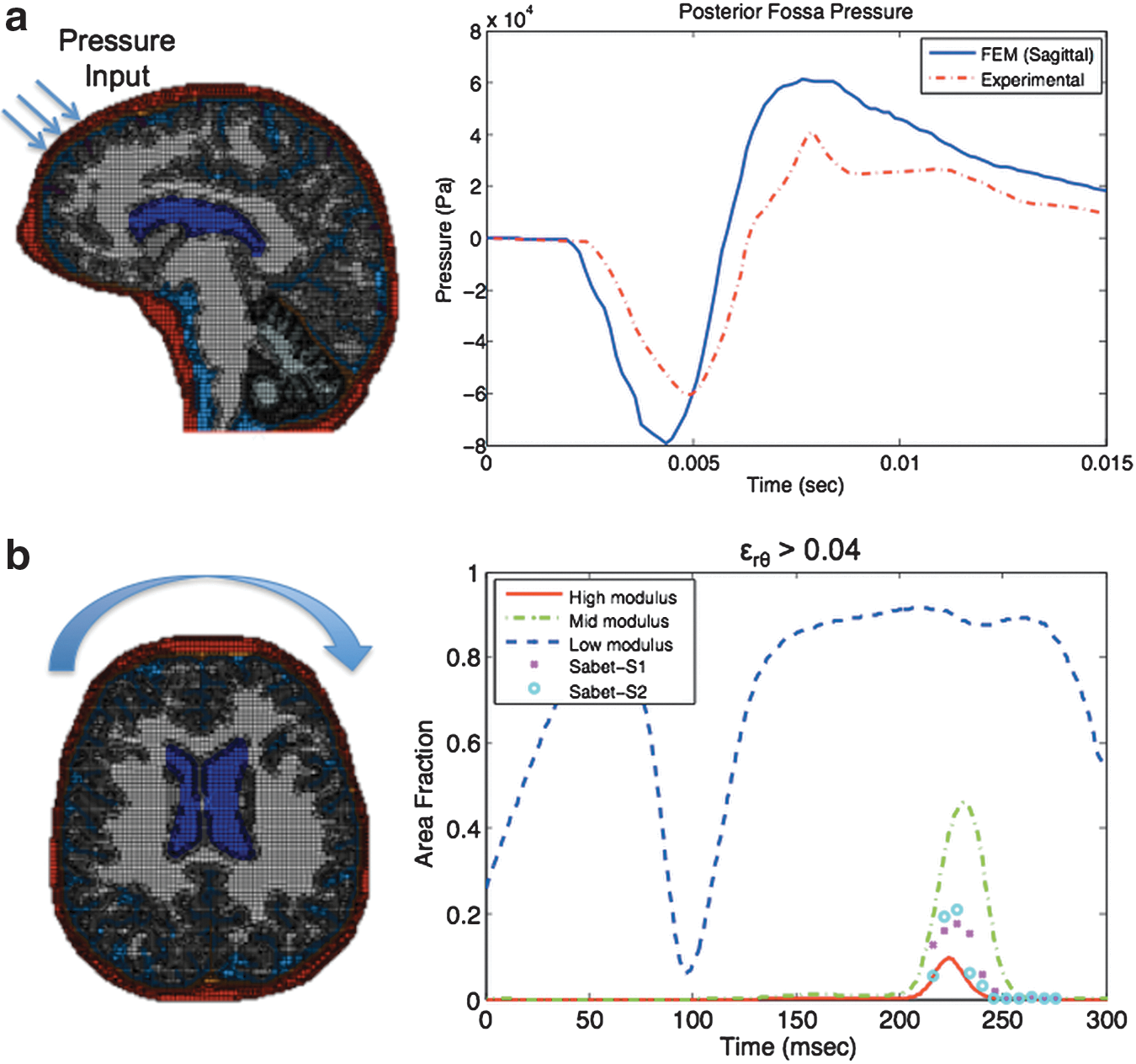
One limitation of the 2-D FE models is that the models cannot capture the complex stress wave interactions that would occur in a 3-D head, which have may have led to this variation in the magnitude of pressure.

We simulated the inertial loading experiment conducted by Sabet et al.³⁸ to validate the deviatoric behavior of the brain tissue in our FE models. This experimental study is unique in that it was performed on human subjects instead of cadavers; therefore, the mechanical response of the tissue was not affected by the tissue degradation that typically occurs in cadaveric studies. In the Sabet study, a mild angular acceleration about the axial plane was imparted to the heads of human subjects, and the resulting shear strain field was determined using tagged MRI. We simulated the experiment by applying an angular rotation about the center of mass of our axial FE model as shown in Figure 6b. The radial-circumferential shear strain, ɛ_rθ, was computed using the three sets of material parameters listed in Table 1, and the area fraction of the brain tissue exceeding a shear strain threshold of 0.04 is plotted in Figure 6b. The simulation results are represented by the dashed and solid lines, and the experimental results are indicated by the markers. The “low modulus” parameters were found to be too compliant, whereas the “mid modulus” and “high modulus” parameters represented the temporal response and distribution of strains the best. Overall, the “high modulus” parameters gave the lowest average percent error in the area fraction (3% for the 0.04 strain threshold) between the simulation and experiments. As a result, this set of material parameters was applied in the following accident reconstruction simulations. Further details of this validation study can be found in the Supplementary Materials.

Accident reconstruction application of model

The validated 2-D finite element models were applied to analyze axonal injury in a real-life injury event. The event that was chosen for the analysis was a well-documented impact to the head of a professional ice hockey player that resulted in concussive injury. The hockey accident was reconstructed using a pneumatic linear impactor and a Hybrid III head and neck form.^39,40 From the accident reconstruction, the acceleration loading histories of the head were obtained, and these loading histories were applied as an input into our finite element models.

Loading condition

The acceleration histories derived from the accident reconstruction were decomposed into components of translational acceleration and angular acceleration about the center of gravity of the head. These accelerations are shown in Figure 7 for an impact speed of 7.5 m/sec. The coordinate system was defined with the x-axis positive in the anterior direction, the y-axis positive toward the right ear, and the z-axis positive in the inferior direction. The maximum magnitude of the linear and angular acceleration components and the peak resultant accelerations are listed in Table 5. The corresponding Head Injury Criterion (HIC₁₅) and Gadd Severity Index (GSI) measures for this impact are 195 and 292, respectively. These values are well below the regulatory limit for serious brain injury according to automotive industry standards.²⁹

FIG. 7.

The applied (a) linear and (b) angular acceleration loading histories are shown for an 7.5 m/sec impact to the head (data provided by Dr. Blaine Hoshizaki). (c) The head coordinate system is defined with the x-axis positive in the anterior direction, the y-axis positive toward the right ear, and the z-axis positive in the inferior direction. Color image is available online at www.liebertonline.com/neu

Table 5.

Maximum Magnitudes of Acceleration for a 7.5 m/Sec Impact

Axis	Linear (g)	Angular (rad/s²)
x	−25.1	6159
y	−84.7	2824
z	−17.9	−8004
Resultant	84.9	8154

The acceleration loading curves from the accident reconstruction were used as inputs in our FE models. As the 2-D FE models can only capture in-plane motions, only the translational and angular acceleration components acting within the plane of each model were considered. For example, the y and z translational components of acceleration and the x component of angular acceleration were applied to the coronal FE model. Although the acceleration histories were acquired for the first 15 msec of the impact, the finite element simulations were performed over a 25 msec time period to give the shear waves enough time to propagate through the brain tissue. The importance of allowing the shear waves enough time to travel through the brain was demonstrated in a study by Chen and Ostoja-Starzewski.²⁵ The accelerations were set to zero after the first 15 msec.

Results

White matter damage

After applying the acceleration loading curves to our FE models, the degree of axonal damage was estimated using the ASI criterion. The predicted damaged regions from the FE analysis are shown in Figure 8. No damage was found in the sagittal model; however, injury was predicted in both the coronal and axial sections, with the greatest degree of damage occurring in the axial section. This large degree of damage in the axial model is attributed to the fact that the maximum magnitude of angular acceleration was applied to this section. Most of the damage occurred at the interface between the white and gray matter in the superficial regions of the white matter, which has been cited to be a common location of DAI.⁴¹ These regions are susceptible to injury because the difference in stiffness between the white and gray matter leads to the development of strain gradients at the interface of these materials.

FIG. 8.

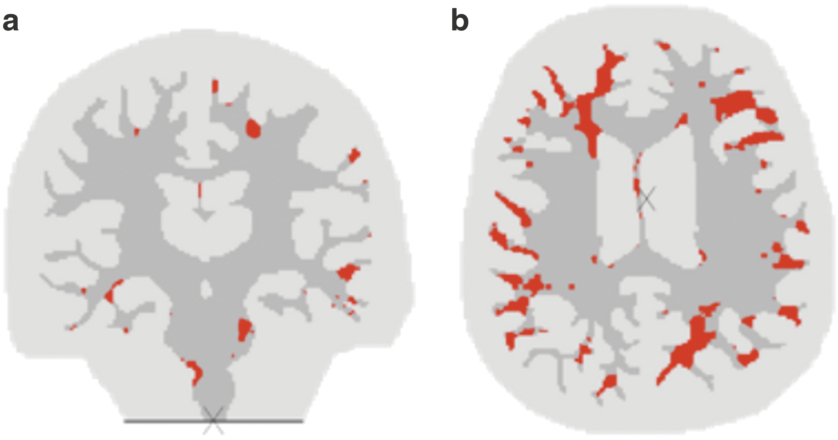
The predicted locations of axonal damage (t=25 msec) are shown in red for (a) the coronal slice and (b) the axial slice. No damage was observed in the sagittal slice model. The white matter is indicated by the dark gray regions. These spatial damage maps are shown in the radiological convention; therefore, the right side of the coronal and axial maps is the left hemisphere of the brain. Color image is available online at www.liebertonline.com/neu

For a given fiber tract, the damage is defined to be 100% if the entire area of the tract exceeds the axonal strain injury threshold of 18% during the course of the simulation. There are 130 labeled structures in the white matter atlas (see Appendix). The percent damage in each one of these structures is plotted for the axial and coronal models (Fig. 9). Note that not all the structures are contained in each one these model sections. To show the temporal accumulation of injury, the tract damage is shown for three different time points of the simulation: 10 msec, 15 msec, and 25 msec. Most of the damage in the coronal slice occurs after the first 15 msec of the loading whereas there is a steady progression of injury in the axial slice. As expected, the total area of damage increases with increasing time.

FIG. 9.

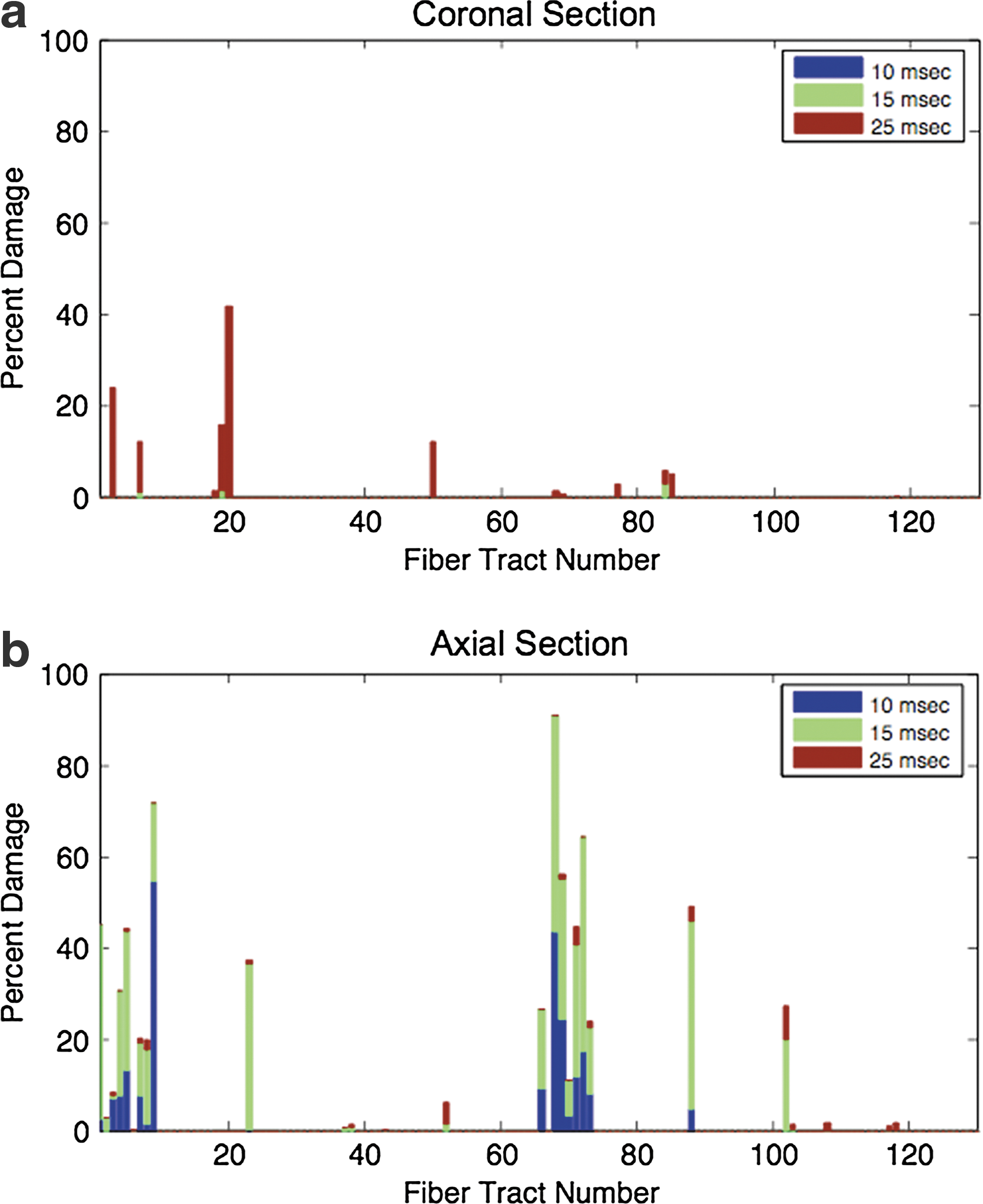
The percent damage in the fiber tracts is plotted against the tract number for (a) the coronal finite element (FE) model and (b) the axial FE model. The damage is plotted at three different time points: 10 msec (blue), 15 msec (green), and 25 msec (red). A table listing the region associated with each tract number can be found in the Appendix. Color image is available online at www.liebertonline.com/neu

The white matter regions with the highest predicted percent of axonal injury are listed in Tables 6 and 7 for the coronal and axial models, respectively. The regions with the maximum damage are located within the middle temporal gyrus (42%) in the coronal section and the superior frontal gyrus (91%) in the axial section. These regions of the brain are responsible for cognitive functions such as self-awareness, spatial awareness, and interpretation of language.^42
–44 Although most of the damage is located within the gyri, axonal injury was also found in the fiber tracts that serve as information pathways in the brain. In the axial slice, the corona radiata was subjected to injury. This fiber tract is responsible for transferring information from the cortex to the lower parts of the brain.⁴⁵ The genu of the corpus callosum was also found to be injured in the axial slice. The corpus callosum facilitates communication between the two cerebral hemispheres of the brain. In the coronal model, damage was predicted in the axons of the middle cerebellar peduncle. This region transfers information between the cortex and the cerebellum, which is highly involved in motor control.⁴⁵ Although we are not clinicians and cannot make a clinical diagnosis, our computations suggest, based on the predicted regions of injury, that the player may have experienced symptoms such as disorientation, difficulty in interpreting language, and, perhaps, even some impairments in motor control. It is known that this specific impact to the head resulted in concussive injury, and as a result of the injury, the hockey player was unable to return to the game for many months. The symptoms predicted from the fiber tract damage analysis correlate well with this type of injury.

Table 6.

White Matter Regions within the Coronal Slice with the Highest Percent of Damage at t=25 Msec

Tract #	Region name	Percent damage (%)
20	Middle temporal gyrus (left)	42
3	Superior frontal gyrus (left)	24
19	Inferior temporal gyrus (left)	16
50	Middle cerebellar peduncle (left)	12
7	Postcentral gyrus (left)	12

Table 7.

White Matter Regions Within the Axial Slice with the Highest Percent of Damage at t=25 Msec

Tract #	Region name	Percent damage (%)
68	Superior frontal gyrus (right)	91
9	Pre-cuneus (left)	72
72	Postcentral gyrus (right)	64
69	Middle frontal gyrus (right)	56
88	Supramarginal gyrus (right)	49
1	Superior parietal lobule (left)	45
71	Precentral gyrus (right)	45
5	Inferior frontal gyrus (left)	44
23	Supramarginal gyrus (left)	37
4	Middle frontal gyrus (left)	31
102	Anterior corona radiata (right)	27
66	Superior parietal lobule (right)	27
73	Angular gyrus (right)	24
7	Postcentral gyrus (left)	20
8	Angular gyrus (left)	20
70	Inferior frontal gyrus (right)	11
3	Superior frontal gyrus (left)	8
52	Genu of corpus callosum (left)	6

Influence of translational and rotational acceleration on the injury response

Angular acceleration has often been cited to be the most common cause of DAI.¹ To study the effect of the translational and rotational components of acceleration on the development of axonal injury, the acceleration loading curves derived for the 7.5 m/sec impact were decomposed into the translational and rotational components. The FE analysis was then conducted for each slice model using either only the translational components of acceleration or only the rotational component of acceleration. The results are shown in Figure 10. It is evident from these spatial damage plots that the rotational component of acceleration dominates the injury response. A negligible amount of axonal damage was found when only the translational components of acceleration were applied to the models; however, with only the application of the rotational acceleration, the distribution of injury closely matches the results from applying both translational and rotational acceleration. This analysis demonstrates the importance of taking angular acceleration into account when developing acceleration-based injury criteria for TBI.

FIG. 10.

The locations of axonal damage (t=25 msec) are shown in red for (a) applied rotational components of acceleration, (b) applied translational components of acceleration, and (c) applied rotational and translational components of acceleration. The coronal results are shown on the left, axial results are in the middle, and sagittal results are on the right. The white matter is indicated by the dark gray regions. The spatial damage maps are shown in the radiological convention; therefore, the right side of the coronal and axial maps is the left hemisphere of the brain. Color image is available online at www.liebertonline.com/neu

In addition, this study demonstrates the importance of incorporating improved neck boundary conditions in computational models of TBI for cases in which the accelerations of the head are unknown. A free boundary condition is often used at the head–neck interface in finite element simulations of head impact; however, with a free boundary condition, the predominant motion of the head is translational and the rotational motion is not captured accurately.²⁵ Without properly capturing the rotational kinematics of the head, the extent of axonal injury cannot be accurately estimated. In our FE analysis, we did not simulate an impact to the head to determine the rotational accelerations, but instead, the accelerations were obtained directly from accident reconstruction data and then applied to our model; therefore, the neck boundary condition was not a contributing factor in determining the extent of axonal injury.

Comparison of ASI criterion with other strain injury criteria

The maximum principal strain and shear strain are commonly used as injury criteria in computational models of TBI. To compare the injury predicted using these strain injury criteria with that predicted by the ASI criterion developed in this work, the acceleration loading curves from the 7.5 m/s impact were applied to the 2-D FE models, and the injury was estimated using the three injury criteria. For the maximum principal strain measure, the white matter regions were assumed to be damaged if the maximum principal strain in the region exceeded a strain threshold of 31%, which is the injury tolerance threshold for mild DAI proposed by Deck and Willinger.² For the shear strain measure, a shear strain threshold of 25% was used to indicate the onset of axonal damage, as proposed by Deck and Willinger.² Similar to the analysis with the ASI criterion, once a region was damaged, it could not become undamaged during the course of the simulation.

The regions predicted to be damaged with the injury criteria are shown in Figure 11 for the axial section. For the injury tolerance thresholds used, the shear strain injury criterion predicted a greater degree of damage than the maximum principal strain and ASI criteria. The shear strain injury criterion predicted damage in ∼62% of the total white matter area whereas both the maximum principal strain and ASI criteria predicted damage in ∼16% of the white matter. Although the total area of predicted damage was similar between the maximum principal strain and ASI criteria, the predicted locations of injury differed between the two criteria (Fig. 11). For example, 63% of the left superior frontal gyrus was predicted to be damaged with the maximum principal strain injury criterion whereas only 8% of this region was predicted to be damaged with the ASI criterion. Without further validating the injury predictions, we cannot state which injury criterion provides a better measure of axonal damage; however, the ASI criterion should more accurately predict the region of injury, as it takes the structure of the white matter into account and is based on a physiologically relevant measure of damage.

FIG. 11.

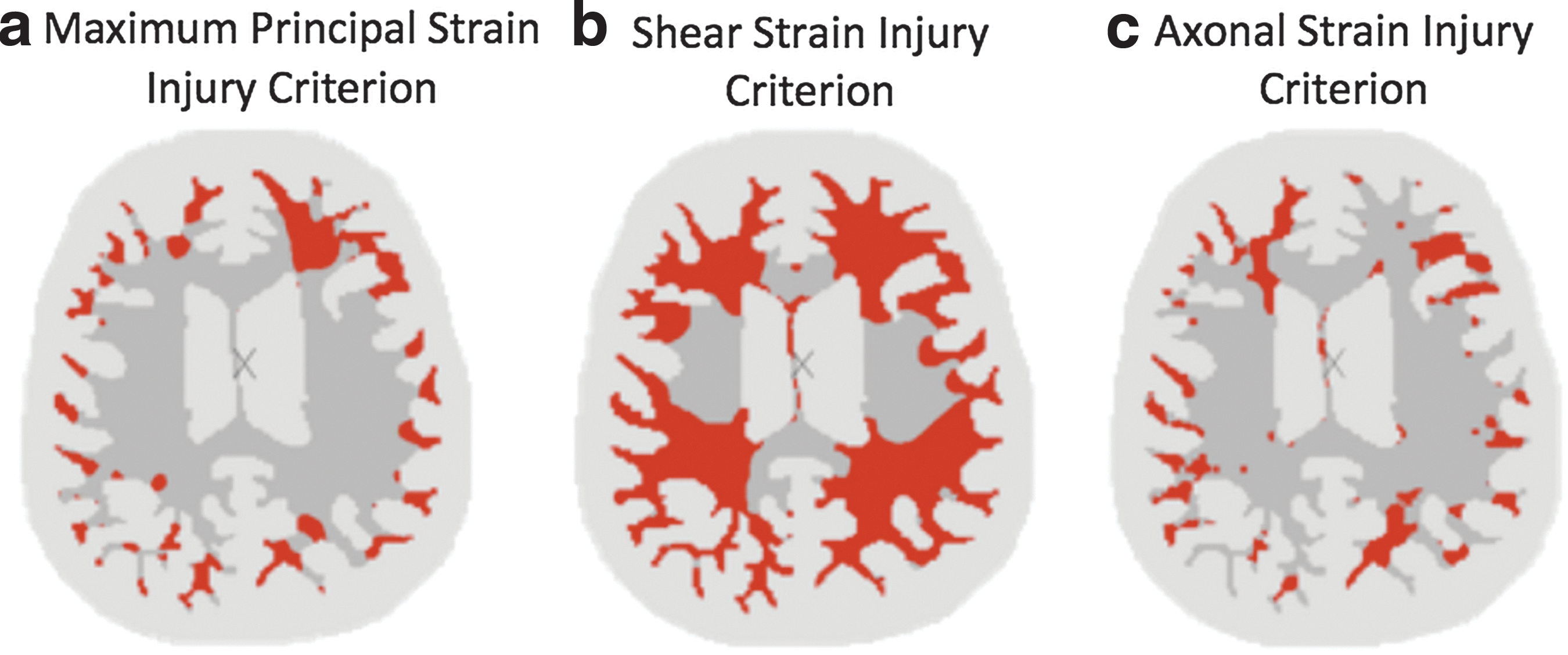
White matter damage was computed using three different injury criteria: (a) maximum principal strain, (b) shear strain, and (c) axonal strain. An injury strain threshold of 31% and 25% was used for the maximum principal strain and shear strain analysis, respectively.² A strain threshold of 18% was used for the axonal strain computation.⁷ The resulting damaged regions using each strain injury criterion are shown in red for the axial section for a 7.5 m/sec impact to the head (t=25 msec). Color image is available online at www.liebertonline.com/neu

Effect of anisotropy on the injury response

The degree of anisotropy in the white matter is controlled through the fiber dispersion parameter, κ. To study the effect of the degree of anisotropy on the injury response, we applied the acceleration loading curves from the 7.5 m/sec impact to the 2-D FE models and varied the fiber dispersion parameter from a value of 0 (i.e., perfectly aligned fibers) to a value of 1/3 (i.e., randomly distributed fibers). The predicted axonal damage is shown in Figure 12 for three different white matter models. In the isotropic model, κ is set equal to 1/3 in all white matter regions. In the transversely isotropic model, κ is set equal to zero, and in the anisotropic HGO model, κ is varied locally based on the fractional anisotropy map as previously described. In all three cases, the gray matter was modeled as isotropic with κ=1/3. Overall, the injury patterns were very similar for the three cases. Both the isotropic model and the HGO model predicted axonal damage in ∼16% of the total white matter area, whereas the transversely isotropic model predicted damage in ∼11% of the white matter. This reduction in the predicted area of damage was caused by the increased stiffness in the fiber direction of the transversely isotropic model. As our model accounted for the fiber orientation through the ASI criterion and the white matter was a weakly anisotropic material, the injury response could be predicted reasonably well with an isotropic model for the white mater. This was also demonstrated in a previous study.⁷ Although the injury can be approximated well with an isotropic model, we chose to retain the higher resolution fiber dispersion data in this study since it did not add a significant computational cost, and the inclusion of anisotropy does lead to some local differences in the predicted location of injury, which can affect the computed degree of axonal damage, especially in smaller fiber tracts.

FIG. 12.

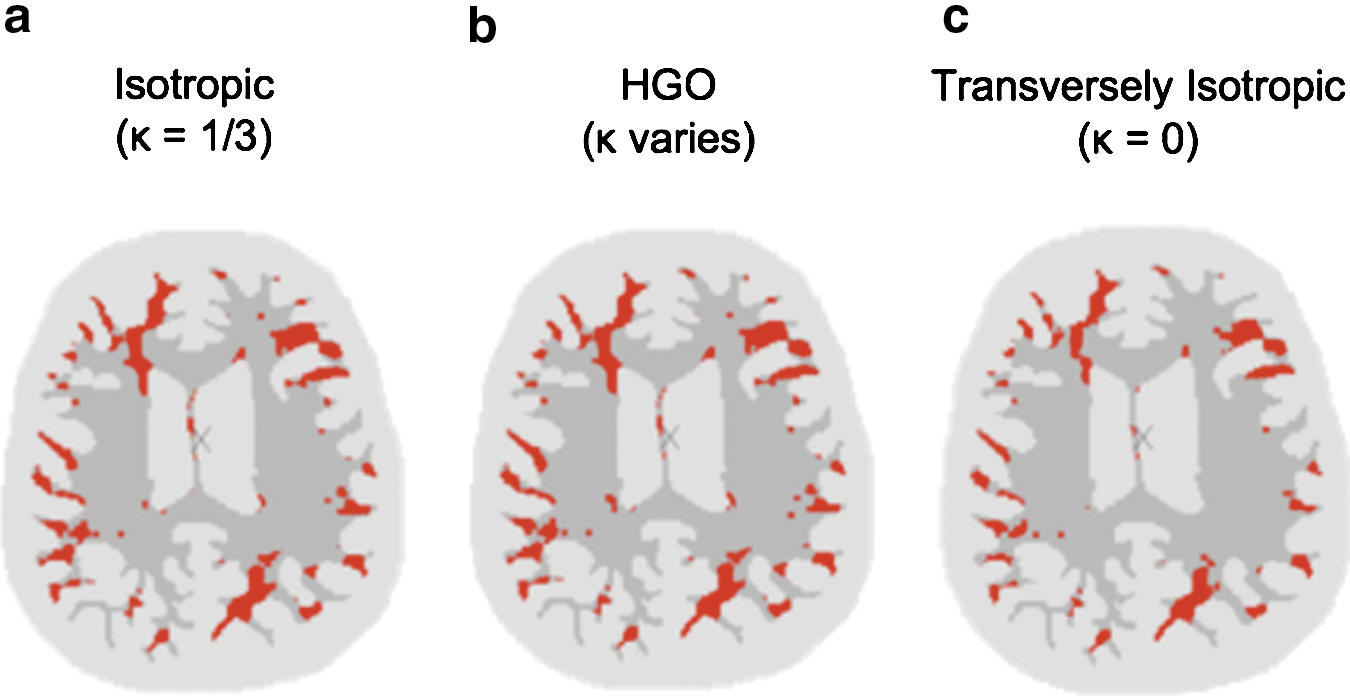
The white matter damage is shown in red for a 7.5 m/sec impact (t=25 msec) using three different fiber dispersion parameters for the white matter: (a) an isotropic model in which κ=1/3, (b) an anisotropic Holzapfel–Gasser–Ogden (HGO) model in which κ is determined locally from the diffusion tensor imaging (DTI) data, and (c) a transversely isotropic model in which κ=0. Color image is available online at www.liebertonline.com/neu

Discussion

In this work, we used an ASI criterion to estimate the degree of axonal damage resulting from inertial loads to the head. Recently, several other groups have also applied an axonal strain measure to predict injury in a computational model.^{13,15,46
–48} The ASI criterion has several advantages over traditionally used tissue-level measures of injury. First and most important, the ASI criterion accounts for the structural orientation of the neural axons in the tissue, whereas other measures of injury do not take this into account. It has been shown that the orientation of the neural axons with respect to the direction of applied loading plays an important role in the development of injury.⁴⁹ Furthermore, our oriented measure of injury is based on an experimental measure of functional damage in an animal model, and therefore it is a physiologically relevant criterion. By accounting for the microstructure of the tissue and the cellular mechanism of injury, the ASI criterion may be a better indicator of neural damage than currently available injury criteria.

For the specific impact case that we analyzed, the regions predicted to be damaged with the ASI criterion correlated well with regions cited to be commonly injured in TBI. Although the 2-D FE models cannot capture the full extent of the axonal injury that would occur in a 3-D head, the fiber tracts predicted to have the greatest degree of damage in our analysis correlated well with the predominant regions of damage identified in studies of concussion. For example, Niogi et al.⁵⁰ measured white matter damage in patients with mild TBI using diffusion tensor imaging, and it was found that the anterior corona radiata was the most commonly damaged region, with 41% of the patients exhibiting axonal damage in this region. In our analysis, the anterior corona radiata was also identified to be significantly damaged because of the inertial loads in the axial plane.

It is important to note that the 2-D models used in this study only consider in-plane accelerations, and out-of-plane accelerations could also lead to injury in these model sections. Furthermore, the percentage of fiber tract damage is based on the area of the fiber tracts contained within each FE model and does not consider the full volume of the tract. Despite these limitations of the 2-D analysis, this work demonstrates the ability of this approach to analyze axonal injury caused by mechanical inertial loads to the head. In future work, this methodology will be applied to 3-D FE head models to analyze injury.

A computational model that provides 3-D analysis of fiber tract damage resulting from direct impact to the head is a valuable tool for investigating the relationship between the impact characteristics and resulting axonal damage, ultimately allowing researchers to identify impact conditions that result in serious head injuries reflecting the location of the axonal damage and subsequent cognitive impairments (Fig. 13). Understanding this relationship provides helmet manufacturers and league officials with valuable information for developing safer helmet technologies and for establishing rules intended to decrease head injuries. This information will shed light on the characteristics of concussive injuries and provide a basis for establishing the character of the injury or injuries, leading to an understanding of the resulting cognitive deficiency and to treatment strategies. It is this research that will connect the event to the injury and ultimately the treatment and outcome. Understanding these relationships is critical in managing the risk of injury, providing an accurate diagnosis, appropriate treatment, and successful outcome.

FIG. 13.

Our computational model for diffuse axonal injury (DAI) can be applied to understand how damage in the neural pathways of the brain leads to the loss of cognitive function. (a) We can reconstruct an impact to the head from a sporting event, in which the impact is documented either through video footage or from accelerometer data. (b) The damage in the neural tracts can be quantified through the use of our computational modeling framework. (c) The damaged regions of the brain can be correlated to the neurological outcome measures from the individual, and a better understanding of functional areas of the brain can be developed. Color image is available online at www.liebertonline.com/neu

As demonstrated in this study, our computational modeling framework for DAI has direct applications in assessing the extent of injury in well-documented sports accidents. As professional sports games are often recorded on high-definition video from multiple angles, the video footage can be used to reconstruct the kinematics of a collision. Furthermore, some sports teams instrument their players' helmets or mouthguards with accelerometers, which can also be used to obtain the accelerations of the head in an impact.^51

–54 Although these methods are still in the validation stage, they offer an excellent approach for directly obtaining the accelerations of an impact. By applying these acceleration loading conditions to our computational model, we can determine the extent of axonal injury in the neural pathways of the brain and identify the fiber tracts with the greatest probability of damage. This type of analysis is especially useful in cases of mild TBI, in which the injury cannot be visualized with medical imaging. The results from the computational analysis could then be used in conjunction with neuropsychological tests to determine the necessary precautions that should be taken to protect the athlete and to help guide treatment measures and rehabilitation strategies. For example, the results could be used to determine whether it is safe for the athlete to resume participation in the sport based on the severity of the injury. This may be critical in protecting athletes against chronic traumatic encephalopathy, which is a degenerative disease that may be found in individuals who experience repeated concussions.⁵⁵ By integrating a computational DAI analysis with a neurophysiological assessment, we can provide better treatment for athletes who sustain concussions during a documented sporting event.

In order for our computational model for DAI to be a viable tool in assessing axonal injury in humans, the performance of the model must be validated against experimental data in future work. Animal models provide a highly controlled experimental platform that could be used to validate the accuracy of the ASI criterion in predicting locations of DAI in the brain.^56

–59 Validation of these injury predictions is a critical next step before this modeling approach can be applied to the clinical setting. To improve the predictive capability of the model, the ASI criterion can also be extended to incorporate the effect of strain rate on the injury response. In vitro studies, such as those by Elkin and Morrison,⁶⁰ have shown that stretch-induced neural cell death is not only a function of strain, but also a function of strain rate. Although further in vitro studies should be conducted to better understand the relationship between strain, strain rate, and the injury response, the incorporation of the rate effects into the measure for axonal injury may improve the injury predictions.

Conclusion

We have developed a conceptual modeling framework that can be used to predict the degree and location of DAI in a computational head model. The ability to couple the cellular mechanisms of axonal damage with the mechanical loads on the head at the macroscale makes our computational modeling platform a useful platform for studying DAI. Our computational modeling framework can be applied to develop new standards and protocols to protect against DAI and assess the extent of DAI in well-documented sports accidents. In the clinical setting, it can be used to provide doctors with valuable information regarding the common locations of axonal injury in the brain, to guide the treatment of TBI. This work offers an innovative modeling framework for diffuse axonal injury and provides a basis upon which future research can build.

Footnotes

Acknowledgments

We gratefully acknowledge Dr. Susumu Mori at the Johns Hopkins University School of Medicine for providing the medical imaging data used in this study, and Dr. Reuben Kraft at the Army Research Laboratory (ARL) for providing access to ARL's High Performance Computing Systems. This work was supported by a National Science Foundation Graduate Research Fellowship and by the Center for Advanced Metallic and Ceramic Systems. Dr. Wright developed the modeling framework, conducted the computational analysis, and prepared the manuscript, with assistance and advice on formulation from her doctoral advisor, Dr. Ramesh. Mr. Post provided the accelerometer data and provided clarification on the accident reconstruction procedure, and Dr. Hoshizaki provided insight on applications.

Author Disclosure Statement

No competing financial interests exist.

Appendix.

Segmented Brain Tissue Structures in Single-Subject White Matter Atlas ³⁶

Tract #	Region name	Tract #	Region name
1	Superior parietal lobule (left)	66	Superior parietal lobule (right)
2	Cingulate gyrus (left)	67	Cingulate gyrus (right)
3	Superior frontal gyrus (left)	68	Superior frontal gyrus (right)
4	Middle frontal gyrus (left)	69	Middle frontal gyrus (right)
5	Inferior frontal gyrus (left)	70	Inferior frontal gyrus (right)
6	Precentral gyrus (left)	71	Precentral gyrus (right)
7	Postcentral gyrus (left)	72	Postcentral gyrus (right)
8	Angular gyrus (left)	73	Angular gyrus (right)
9	Pre-cuneus (left)	74	Pre-cuneus (right)
10	Cuneus (left)	75	Cuneus (right)
11	Lingual gyrus (left)	76	Lingual gyrus (right)
12	Fusiform gyrus (left)	77	Fusiform gyrus (right)
13	Parahippocampal gyrus (left)	78	Parahippocampal gyrus (right)
14	Superior occipital gyrus (left)	79	Superior occipital gyrus (right)
15	Inferior occipital gyrus (left)	80	Inferior occipital gyrus (right)
16	Middle occipital gyrus (left)	81	Middle occipital gyrus (right)
17	Entorhinal area (left)	82	Entorhinal area (right)
18	Superior temporal gyrus (left)	83	Superior temporal gyrus (right)
19	Inferior temporal gyrus (left)	84	Inferior temporal gyrus (right)
20	Middle temporal gyrus (left)	85	Middle temporal gyrus (right)
21	Lateral fronto-orbital gyrus (left)	86	Lateral fronto-orbital gyrus (right)
22	Middle fronto-orbital gyrus (left)	87	Middle fronto-orbital gyrus (right)
23	Supramarginal gyrus (left)	88	Supramarginal gyrus (right)
24	Gyrus rectus (left)	89	Gyrus rectus (right)
25	Insular (left)	90	Insular (right)
26	Amygdala (left)	91	Amygdala (right)
27	Hippocampus (left)	92	Hippocampus (right)
28	Cerebellum (left)	93	Cerebellum (right)
29	Corticospinal tract (left)	94	Corticospinal tract (right)
30	Inferior cerebellar peduncle (left)	95	Inferior cerebellar peduncle (right)
31	Medial lemniscus (left)	96	Medial lemniscus (right)
32	Superior cerebellar peduncle (left)	97	Superior cerebellar peduncle (right)
33	Cerebral peduncle (left)	98	Cerebral peduncle (right)
34	Anterior limb of internal capsule (left)	99	Anterior limb of internal capsule (right)
35	Posterior limb of internal capsule (left)	100	Posterior limb of internal capsule (right)
36	Posterior thalamic radiation (including optic radiation) (left)	101	Posterior thalamic radiation (including optic radiation) (right)
37	Anterior corona radiata (left)	102	Anterior corona radiata (right)
38	Superior corona radiata (left)	103	Superior corona radiata (right)
39	Posterior corona radiata (left)	104	Posterior corona radiata (right)
40	Cingulum (cingulated gyrus) (left)	105	Cingulum (cingulated gyrus) (right)
41	Cingulum (hippocampus) (left)	106	Cingulum (hippocampus) (right)
42	Fornix (cres)/Stria terminalis (cannot be resolved with current resolution) (left)	107	Fornix (cres)/Stria terminalis (cannot be resolved with current resolution) (right)
43	Superior longitudinal fasciculus (left)	108	Superior longitudinal fasciculus (right)
44	Superior fronto-occipital fasciculus (could be a part of anterior internal capsule) (left)	109	Superior fronto-occipital fasciculus (could be a part of anterior internal capsule) (right)
45	Inferior fronto-occipital fasciculus (left)	110	Inferior fronto-occipital fasciculus (right)
46	Sagittal stratum (include interior longitudinal fasciculus and inferior front-occipital fasciculus) (left)	111	Sagittal stratum (include interior longitudinal fasciculus and inferior front-occipital fasciculus) (right)
47	External capsule (left)	112	External capsule (right)
48	Uncinate fasciculus (left)	113	Uncinate fasciculus (right)
49	Pontine crossing tract (a part of MCP) (left)	114	Pontine crossing tract (a part of MCP) (right)
50	Middle cerebellar peduncle (left)	115	Middle cerebellar peduncle (right)
51	Fornix (columns and body of fornix) (left)	116	Fornix (columns and body of fornix) (right)
52	Genu of corpus callosum (left)	117	Genu of corpus callosum (right)
53	Body of corpus callosum (left)	118	Body of corpus callosum (right)
54	Splenium of corpus callosum (left)	119	Splenium of corpus callosum (right)
55	Retrolenticular part of internal capsule (left)	120	Retrolenticular part of internal capsule (right)
56	Red nucleus (left)	121	Red nucleus (right)
57	Substancia nigra (left)	122	Substancia nigra (right)
58	Tapatum (left)	123	Tapatum (right)
58	Caudate nucleus (left)	124	Caudate nucleus (right)
60	Putamen (left)	125	Putamen (right)
61	Thalamus (left)	126	Thalamus (right)
62	Globus pallidus (left)	127	Globus pallidus (right)
63	Midbrain (left)	128	Midbrain (right)
64	Pons (left)	129	Pons (right)
65	Medulla (left)	130	Medulla (right)

References

Smith

D.H.

, Meaney

D.F.

2000. Axonal damage in traumatic brain injury. Neuroscientist, 6:483–495

Deck

, Willinger

2008. Improved head injury criteria based on head FE model. International Journal of Crashworthiness, 13:667–678.

Raul

J.S.

, Deck

, Willinger

, Ludes

2008. Finite-element models of the human head and their applications in forensic practice. Int. J. Legal Med., 122:359–366.

Voo

, Kumaresan

, Pintar

F.A.

, Yoganandan

, Sances

Jr . 1996. Finite-element models of the human head. Med. Biol. Eng. Comput., 34:375–381.

Chatelin

, Constantinesco

, Willinger

2010. Fifty years of brain tissue mechanical testing: from in vitro to in vivo investigations. Biorheology, 47:255–276.

Kyriacou

S.K.

, Mohamed

, Miller

, Neff

2002. Brain mechanics for neurosurgery: modeling issues. Biomech. Model. Mechanobiol., 1:151–164.

Wright

R.M.

, Ramesh

K.T.

2011. An axonal strain injury criterion for traumatic brain injury. Biomech. Model. Mechanobiol., 11:245–260.

Feist

, Gugler

, Arregui–Dalmases

, del Pozo de Dios

, Lopez–Valdes

, Deck

, Willinger

2009. Pedestrian collisions with flat-fronted vehicles: Injury patterns and importance of rotational accelerators as a predictor for traumatic brain injury (TBI) 21st International Conference on the Enhanced Safety of Vehicles (ESV), National Highway Traffic Safety Administration, Stutgart: Germany, 1–19.

Morrison

3rd , Elkin

B.S.

, Dolle

J.P.

, Yarmush

M.L.

2011. In vitro models of traumatic brain injury. Annu. Rev. Biomed. Eng., 13:91–126.

10.

Morrison

3rd , Saatman

K.E.

, Meaney

D.F.

, McIntosh

T.K.

1998. In vitro central nervous system models of mechanically induced trauma: a review. J. Neurotrauma, 15,11:911–928.

11.

Hrapko

, van Dommelen

J.A.W.

, Peters

G.W.M.

, Wismans

J.S.H.M.

2008. The influence of test conditions on characterization of the mechanical properties of brain tissue. J. Biomech. Eng., 130:663–676.

12.

Gasser

T.C.

, Ogden

R.W.

, Holzapfel

G.A.

2006. Hyperelastic modelling of arterial layers with distributed collagen fibre orientations. J. R. Soc. Interface, 3:15–35.

13.

Cloots

R.J.

, van Dommelen

J.A.

, Geers

M.G.

2011. A tissue-level anisotropic criterion for brain injury based on microstructural axonal deformation. J. Mech. Behav. Biomed. Mater., 5:41–52.

14.

Cloots

R.J.

, van Dommelen

J.A.

, Nyberg

, Kleiven

, Geers

M.G.

2011. Micromechanics of diffuse axonal injury: Influence of axonal orientation and anisotropy. Biomech. Model. Mechanobiol., 10,3:413–422.

15.

Colgan

N.C.

, Gilchrist

M.D.

, Curran

K.M.

2010. Applying DTI white matter orientations to finite element head models to examine diffuse TBI under high rotational accelerations. Prog. Biophys. Mol. Biol., 103:304–309.

16.

Merodio

, Ogden

R.W.

2005. Mechanical response of fiber-reinforced incompressible non-linearly elastic solids. Int. J. Non Linear Mech., 40:213–227.

17.

Bain

A.C.

, Meaney

D.F.

2000. Tissue-level thresholds for axonal damage in an experimental model of central nervous system white matter injury. J. Biomech. Eng., 122:615–622.

18.

Tamura

, Nagayama

, Matsumoto

2006. Measurement of nerve fiber strain in brain tissue subjected to uniaxial stretch (comparison between local strain of nerve fiber and global strain of brain tissue) J. Biomech. Sci. Eng., 1:304–315.

19.

Le Bihan

, Mangin

J.-F.

, Poupon

, Clark

C.A.

, Pappata

, Molko

, Chabriat

2001. Diffusion tensor imaging: concepts and applications. J. Magn. Reson. Imaging, 13:534–546

20.

Bammer

, Acar

, Moseley

M.E.

2003. In vivo MR tractography using diffusion imaging. Eur. J. Radiol., 45:223–234.

21.

Basser

P.J.

, Pierpaoli

1996. Microstructural and physiological features of tissues elucidated by quantitative-diffusion-tensor MRI. J. Magn. Reson. B, 111:209–219.

22.

Niogi

S.N.

, Mukherjee

2010. Diffusion tensor imaging of mild traumatic brain injury. J. Head Trauma Rehabil., 25:241–255.

23.

Yushkevich

P.A.

, Piven

, Hazlett

H.C.

, Smith

R.G.

, Ho

, Gee

J.C.

, Gerig

2006. User-guided 3d active contour segmentation of anatomical structures: significantly improved efficiency and reliability. Neuroimage, 31:1116–1128.

24.

Velardi

, Fraternali

, Angelillo

2006. Anisotropic constitutive equations and experimental tensile behavior of brain tissue. Biomech. Model. Mechanobiol., 5:53–61.

25.

Chen

, Ostoja–Starzewski

2010. MRI-based finite element modeling of head trauma: Spherically focusing shear waves. Acta Mechanica, 213:155–167.

26.

El Sayed

, Mota

, Fraternali

, Ortiz

2008. Biomechanics of traumatic brain injury. Comput. Methods Appl. Mech. Eng., 197:4692–4701.

27.

Kleiven

2007. Predictors for traumatic brain injuries evaluated through accident reconstructions. Stapp Car Crash J., 51:81–114

28.

Taylor

P.A.

, Ford

C.C.

2009. Simulation of blast-induced early-time intracranial wave physics leading to traumatic brain injury. J. Biomech. Eng., 131:061007-1–61007-11.

29.

Zhang

L.Y.

, Yang

K.H.

, King

A.I.

2004. A proposed injury threshold for introduction mild traumatic brain injury. J. Biomech. Eng., 126:226–236.

30.

Willinger

, Kang

H.S.

, Diaw

1999. Three-dimensional human head finite-element model validation against two experimental impacts. Ann. Biomed. Eng., 27:403–410.

31.

Zhang

L.Y.

, Yang

K.H.

, King

A.I.

2001. Comparison of brain responses between frontal and lateral impacts by finite element modeling. J. Neurotrauma, 18:21–30.

32.

Zhang

, Green

M.A.

, Sinkus

, Bilston

L.E.

2011. Viscoelastic properties of human cerebellum using magnetic resonance elastography. J. Biomech., 44:1909–1913.

33.

Monson

K.L.

, Goldsmith

, Barbaro

N.M.

, Manley

G.T.

2003. Axial mechanical properties of fresh human cerebral blood vessels. J. Biomech. Eng., 125:288–294.

34.

Itoh

, Hamashima

, Murata

, Kato

2002. Determination of jwl parameters from underwater explosion test. 12th International Detonation Symposium, San Diego, CA.

35.

Wittek

, Omori

2003. Parametric study of effects of brain-skull boundary conditions and brain material properties on responses of simplified finite element brain model under angular acceleration impulse in sagittal plane. JSME International Journal, Series C:Mechanical Systems, Machine Elements and Manufacturing, 46:1388–1399.

36.

Zhang

, Zhang

, Oishi

, Faria

A.V.

, Jiang

, Li

, Akhter

, Rosa–Neto

, Pike

G.B.

, Evans

, Toga

A.W.

, Woods

, Mazziotta

J.C.

, Miller

M.I.

, van Zijl

P.C.

, Mori

2010. Atlas-guided tract reconstruction for automated and comprehensive examination of the white matter anatomy. Neuroimage, 52:1289–1301.

37.

Nahum

A.M.

, Smith

R.G.

, Ward

C.C.

1977. Intracranial Pressure Dynamics During Head Impact. Society of Automotive Engineers: Warrendale, PA.

38.

Sabet

A.A.

, Christoforou

, Zatlin

, Genin

G.M.

, Bayly

P.V.

2008. Deformation of the human brain induced by mild angular head acceleration. J. Biomech., 41:307–315.

39.

Post

, Oeur

, Hoshizaki

, Gilchrist

M.D.

2011. Examination of the relationship between peak linear and angular accelerations to brain deformation metrics in hockey helmet impacts. Comput. Methods. Biomech. Biomed. Engin., Dec 21[Epub ahead of print]

40.

Walsh

E.S.

, Rousseau

, Hoshizaki

T.B.

2011. The influence of impact location and angle on the dynamic impact response of a hybrid III headform. Sports Engineering, 13:135–143.

41.

Gaetz

2004. The neurophysiology of brain injury. Clin Neurophysiol, 115:4–18.

42.

Bottini

, Corcoran

, Sterzi

, Paulesu

, Schenone

, Scarpa

, Frackowiak

R.S.J.

, Frith

C.D.

1994. The role of the right-hemisphere in the interpretation of figurative aspects of language – a positron emission tomography activation study. Brain, 117:1241–1253.

43.

Goldberg

I.I.

, Harel

, Malach

2006. When the brain loses its self: Prefrontal inactivation during sensorimotor processing. Neuron, 50:329–339.

44.

Karnath

H.O.

, Ferber

, Himmelbach

2001. Spatial awareness is a function of the temporal not the posterior parietal lobe. Nature, 411:950–953.

45.

Mori

, Oishi

, Jiang

H.Y.

, Jiang

, Li

, Akhter

, Hua

K.G.

, Faria

A.V.

, Mahmood

, Woods

, Toga

A.W.

, Pike

G.B.

, Neto

P.R.

, Evans

, Zhang

J.Y.

, Huang

, Miller

M.I.

, Zijl

, Mazziotta

2008. Stereotaxic white matter atlas based on diffusion tensor imaging in an icbm template. Neuroimage, 40:570–582.

46.

Cloots

R.J.

, van Dommelen

J.A.

, Kleiven

, Geers

M.G.

2012. Multi-scale mechanics of traumatic brain injury: predicting axonal strains from head loads. Biomech Model Mechanobiol., Mar 21[Epub ahead of print]

47.

Kraft

R.H.

, McKee

P.J.

, Dagro

A.M.

, Grafton

S.T.

2012. Combining the finite element method with structural connectome-based analysis for modeling neurotrauma: connectome neurotrauma mechanics. PLoS Comput. Biol., 8:e1002619.

48.

Chatelin

, Deck

, Renard

, Kremer

, Heinrich

, Armspach

J.P.

, Willinger

2011. Computation of axonal elongation in head trauma finite element simulation. J. Mech. Behav. Biomed. Mater., 4:1905–1919.

49.

LaPlaca

M.C.

, Cullen

D.K.

, McLoughlin

J.J.

, Cargill

R.S.

2005. High rate shear strain of three-dimensional neural cell cultures: a new in vitro traumatic brain injury model. Journal of Biomechanics, 38:1093–1105.

50.

Niogi

S.N.

, Mukherjee

, Ghajar

, Johnson

, Kolster

R.A.

, Sarkar

, Lee

, Meeker

, Zimmerman

R.D.

, Manley

G.T.

, McCandliss

B.D.

2008. Extent of microstructural white matter injury in postconcussive syndrome correlates with impaired cognitive reaction time: a 3T diffusion tensor imaging study of mild traumatic brain injury. A.J.N.R. Am. J. Neuroradiol., 29:967–973.

51.

Greenwald

R.M.

, Gwin

J.T.

, Chu

J.J.

, Crisco

J.J.

2008. Head impact severity measures for evaluating mild traumatic brain injury risk exposure. Neurosurgery, 62,4:789–798.

52.

Mihalik

J.P.

, Bell

D.R.

, Marshall

S.W.

, Guskiewicz

K.M.

2007. Measurement of head impacts in collegiate football players: an investigation of positional and event-type differences. Neurosurgery, 61:1229–1235.

53.

Naunheim

R.S.

, Standeven

, Richter

, Lewis

L.M.

2000. Comparison of impact data in hockey, football, and soccer. J. Trauma, 48:938–941.

54.

Rowson

, Brolinson

, Goforth

, Dietter

, Duma

2009. Linear and angular head acceleration measurements in collegiate football. J. Biomech. Eng., 131:061016.

55.

Viano

D.C.

, Casson

I.R.

, Pellman

E.J.

, Zhang

, King

A.I.

, Yang

K.H.

2005. Concussion in professional football: Brain responses by finite element analysis: part 9. Neurosurgery, 57:891–916.

56.

Cernak

2005. Animal models of head trauma. NeuroRx, 2:410–422.

57.

Eucker

S.A.

, Smith

, Ralston

, Friess

S.H.

, Margulies

S.S.

2010. Physiological and histopathological responses following closed rotational head injury depend on direction of head motion. Exp Neurol, 227:79–88.

58.

Raghupathi

, Mehr

M.F.

, Helfaer

M.A.

, Margulies

S.S.

2004. Traumatic axonal injury is exacerbated following repetitive closed head injury in the neonatal pig. J. Neurotrauma, 21:307–316.

59.

Smith

D.H.

, Nonaka

, Miller

, Leoni

, Chen

X.H.

, Alsop

, Meaney

D.F.

2000. Immediate coma following inertial brain injury dependent on axonal damage in the brainstem. J. Neurosurg., 93:315–322.

60.

Elkin

B.S.

, Morrisonm

III . 2007. Region-specific tolerance criteria for the living brain. Stapp Car Crash J., 51:127–138.

Supplementary Material

Please find the following supplemental material available below.

For Open Access articles published under a Creative Commons License, all supplemental material carries the same license as the article it is associated with.

For non-Open Access articles published, all supplemental material carries a non-exclusive license, and permission requests for re-use of supplemental material or any part of supplemental material shall be sent directly to the copyright owner as specified in the copyright notice associated with the article.

0.00 MB

2.49 MB