Estimating Pressure Reactivity Using Noninvasive Doppler-Based Systolic Flow Index

Abstract

The study objective was to derive models that estimate the pressure reactivity index (PRx) using the noninvasive transcranial Doppler (TCD) based systolic flow index (Sx_a) and mean flow index (Mx_a), both based on mean arterial pressure, in traumatic brain injury (TBI). Using a retrospective database of 347 patients with TBI with intracranial pressure and TCD time series recordings, we derived PRx, Sx_a, and Mx_a. We first derived the autocorrelative structure of PRx based on: (A) autoregressive integrative moving average (ARIMA) modeling in representative patients, and (B) within sequential linear mixed effects (LME) models with various embedded ARIMA error structures for PRx for the entire population. Finally, we performed sequential LME models with embedded PRx ARIMA modeling to find the best model for estimating PRx using Sx_a and Mx_a. Model adequacy was assessed via normally distributed residual density. Model superiority was assessed via Akaike Information Criterion (AIC), Bayesian Information Criterion (BIC), log likelihood (LL), and analysis of variance testing between models. The most appropriate ARIMA structure for PRx in this population was (2,0,2). This was applied in sequential LME modeling. Two models were superior (employing random effects in the independent variables and intercept): (A) PRx ∼ Sx_a, and (B) PRx ∼ Sx_a + Mx_a. Correlation between observed and estimated PRx with these two models was: (A) 0.794 (p < 0.0001, 95% confidence interval (CI) = 0.788–0.799), and (B) 0.814 (p < 0.0001, 95% CI = 0.809–0.819), with acceptable agreement on Bland-Altman analysis. Through using linear mixed effects modeling and accounting for the ARIMA structure of PRx, one can estimate PRx using noninvasive TCD-based indices. We have described our first attempts at such modeling and PRx estimation, establishing the strong link between two aspects of cerebral autoregulation: measures of cerebral blood flow and those of pulsatile cerebral blood volume. Further work is required to validate.

Introduction

The application of continuous monitoring of cerebrovascular autoregulatory capacity in traumatic brain injury (TBI) has increased in popularity slowly within the intensive care unit (ICU) for patients with moderate and severe TBI.^1,2 This is accomplished typically through calculating the moving correlation between fluctuations in slow waves of a marker of pulsatile cerebral blood volume (CBV)/cerebral blood flow (CBF) and a driving pressure to forward flow, such as mean arterial pressure (MAP) or cerebral perfusion pressure (CPP).³ In general, positive values are believed to represent potentially “impaired” autoregulatory capacity, while negative values potentially represent “intact” autoregulation.³ These types of indices have received support even from recent consensus statements on multi-modal monitoring (MMM) in TBI.^2,4

The pressure reactivity index (PRx), the correlation between intracranial pressure (ICP) and MAP, is the one continuous measure of autoregulatory capacity that has received the most attention in the TBI population.³ Numerous studies have been published linking abnormal PRx values to poor outcome in TBI.^3,5,6 Further, thresholds associated with six-month outcomes have been defined for PRx in the TBI population.⁷ Finally, PRx is one of only two indices that have been validated in an animal model against the lower limit of the Lassen autoregulatory curve.⁸

Despite the promising nature of PRx, the major limitation in its acquisition is the need for an invasive measure of ICP. Using near infrared spectroscopy techniques, similar indices have been proposed.^9,10 Other noninvasive autoregulatory indices based on transcranial Doppler (TCD) exist, including: mean flow index (Mx_a = correlation between TCD-based mean flow velocity [FVm] and MAP) and systolic flow index (Sx_a = correlation between TCD-based systolic flow velocity [FVs] and MAP).^5,11 These TCD-derived indices display a positive linear relationship with PRx.^5,11 In addition, recently we have been able to show, in three separate patient populations, the robust statistical covariance and co-clustering of the noninvasively derived Sx_a with the invasively derived PRx.^12
–14 Thus, the question remains: Can we estimate PRx using noninvasive TCD-based autoregulatory indices?

The main issues with modeling PRx is the fact that the high frequency data used are autocorrelated, violating the assumption of statistical independence implicit in simple regression techniques and limiting the literature in this area to date. Our goal was to provide, for the first time, a noninvasive method of estimating PRx using formal time series analysis and linear mixed effects modeling, assessing the calibration with TCD-based techniques.

Methods

Patient population

We used a large retrospective database of patients with TBI who had simultaneous TCD and ICP recording. All high frequency signals from monitoring devices were archived prospectively between January 1992 up to and including September 2011, with all patients being admitted to the neurosciences critical care unit (NCCU) at Addenbrooke's Hospital, Cambridge. The TCD-based cerebral blood flow velocity (CBFV), ICP and arterial blood pressure (ABP) were recorded simultaneously and linked in time series. We accessed this database retrospectively for the purpose of this study. This patient population has been reported in full, or in part, within previous publications from our group.^12
–14

This population is the identical population to that described within our recent publication on the covariance structure of Sx_a and PRx.¹³ All patients included had mild to severe TBI, with those with mild TBI experiencing clinical deterioration, leading to the need for ICU admission for MMM and subsequent ICP monitor insertion solely for clinical purposes. All ICP monitoring was conducted based on the standard suggested population for invasive ICP monitoring within the Brain Trauma Foundation Guidelines.¹⁴ As described previously, treatments received during their ICU stay included standard ICP-directed therapy (i.e., goal less than 20 mm Hg) and a CPP goal of greater than 60 mm Hg.

Similar to our previous publication on covariance,¹³ we were interested only in continuous recording lengths of 30 min or longer for use in linear mixed effects (LME) modeling of PRx. A total of 410 recordings from 347 patients was included.

Ethics

Because this study was a retrospective analysis of a prospectively maintained database cohort and monitoring was conducted as part of standard NCCU patient care using an anonymized database, formal patient or proxy consent was not required. All demographics and physiological data were collected prospectively during time of admission and entered into the database in a fully anonymized fashion, negating the need to reaccess clinical records.

Signal acquisition

The ABP, ICP, and TCD-based CBFV were recorded simultaneously in all patients and were recorded in the same way reported by our previous publications.^12,13,15 The ABP was obtained through either radial or femoral arterial lines connected to pressure transducers (Baxter Healthcare Corp. CardioVascular Group, Irvine, CA), zeroed at the level of the tragus. The ICP was acquired via an intraparenchymal strain gauge probe (Codman ICP MicroSensor; Codman & Shurtleff Inc., Raynham, MA), also zeroed at the level of the tragus. The zeroing levels for both ABP and ICP were conducted in this fashion to provide as accurate an assessment of intracranial CPP as possible. It is acknowledged that zeroing the ABP at the level of the tragus (as opposed to the right atrium) leads to ABP values lower than actual systemic pressures (depending on patient position); however, this provides a more accurate reflection of cerebral vascular pressure—hence, what we believe to represent a more accurate CPP.

The PRx is not impacted by this zeroing level, because it represents the correlation and phase shift between slow-wave fluctuations in ICP and MAP and is thus both theoretically and mathematically independent of the absolute magnitude of the individual values of ICP and MAP. Further, the majority of the PRx literature in TBI to date is based on ICP and ABP signals acquired with zeroing at the tragus.

The TCD assessment of the middle cerebral artery (MCA) CBFV was conducted via Doppler Box (DWL Compumedics, Singen, Germany) or Neuroguard (Medasonic, Fremont, CA). TCD was conducted typically on the right MCA only, ipsilateral to the ICP monitor. In those with poor right-sided transtemporal windows for TCD, the left-sided MCA was recorded. A minority of patients had simultaneous bilateral TCD recordings, and for these we utilized the right-sided signal for further processing and analysis purposes, given this was typically ipsilateral to the ICP monitor.

All recorded signals were digitized via an A/D converters (DT9801 or DT9803; Data Translation, Marlboro, MA), sampled at frequency of 50 Hz or higher, using ICM+ software (Cambridge Enterprise Ltd, Cambridge, UK, http://icmplus.neurosurg.cam.ac.uk, or its predecessor ICM/WREC). Signal artifact was removed before further processing or analysis via a mix of manual and automatic approaches within ICM+.

Signal processing

Post-acquisition processing of the above described signals was conducted utilizing ICM+ software, similar to the previous study.¹³ The CPP was determined as: CPP = MAP – ICP. The FVs was determined by calculating the maximum flow velocity (FV) over a 1.5-sec window, updated every second. Diastolic flow velocity (FVd) was calculated using the minimum FV over a 1.5-sec window, updated every second. The FVm was calculated using average FV over a 10-sec window, updated every 10 sec (i.e., not data overlap). Ten second moving averages (updated every 10 sec to avoid data overlap) were calculated for all recorded signals: ICP, ABP (which produced MAP), CPP, FVm, FVs, and FVd.

Autoregulation indices

For PRx, a moving Pearson correlation coefficient was calculated between ICP and MAP, using 30 consecutive 10-sec windows (i.e., 5 min of data), with an update period of every minute. Similarly, TCD-based Mx_a was derived using a moving Pearson correlation between FVm and MAP, while Sx_a was derived using FVs and MAP. Finally, we also derived diastolic flow index (Dx_a) based on the moving correlation between FVd and MAP.

Statistics

Minute-by-minute time series data were utilized for the entirety of the analysis described below. Statistical significance was set at an alpha of less than 0.05. All statistical analysis was conducted using R statistical software (R Core Team [2016]. R: A language and environment for statistical computing. R Foundation for Statistical Computing, Vienna, Austria. URL https://www.R-project.org/). The following packages were used during the analysis: dplyr, ggplot2, ggthemes, tseries, forecast, lubridate, and lme4.

The statistical methods sections to follow will outline the techniques employed to: (A) estimate the autocorrelative structure of PRx in time series, (B) estimate PRx using noninvasive TCD indices of cerebrovascular reactivity via application of LME modeling¹⁶ (with embedded PRx autoregressive integrative moving average [ARIMA] error structure) to, and (C) assess the correlation and agreement between model-based estimated PRx and the observed PRx values.

Autocorrelative structure of PRx

Before being able to model PRx using TCD-based indices, it was necessary to determine the autocorrelation structure of PRx. We used ARIMA modeling of PRx to determine: the autoregressive structure of order “p”, the differencing factor or order “d”, and the moving average component of order “q”, commonly denoted “(p,d,q)”. The autoregressive structure refers to the dependence of PRx at time t (denoted PRx_t) on previous measures of PRx (i.e., called lags), say, at time t-1 (i.e., PRx_t-1), and so forth (i.e., say to PRx_t-p), with the order “p” indicating how many previous PRx measures PRx_t is dependent on. The differencing component refers to the need to make a nonstationary signal stationary, with seasonal or trending structure within a time series indicating nonstationary character.

Stationarity is defined as the presence of a stable variance, autocorrelative structure, and mean over time. Stationarity can be introduced by differencing previous PRx measures from current measures, thus removing seasonality or trending structure to a time series and allowing further modeling to occur. The differencing order “d” refers to how many previous terms should be included in the differencing process. Finally, the moving average term refers to the need to include the error in the model at time t (i.e., e_t) based on its association in previous measured error terms (i.e., e_t-q). The order “q” for the moving average component refers to how many previous error terms are to be included within the ARIMA model. Assuming stationarity (i.e., no “d” order), a general autoaggressive moving average (ARMA) model can be represented by the following formula: \documentclass{aastex}\usepackage{amsbsy}\usepackage{amsfonts}\usepackage{amssymb}\usepackage{bm}\usepackage{mathrsfs}\usepackage{pifont}\usepackage{stmaryrd}\usepackage{textcomp}\usepackage{portland, xspace}\usepackage{amsmath, amsxtra}\usepackage{upgreek}\pagestyle{empty}\DeclareMathSizes{10}{9}{7}{6}\begin{document} \begin{align*}{ \rm{P}}{{ \rm{R}}_{{ \rm{Xt}}}} = { \rm{C}} + { \varepsilon _t} + \Sigma _{i = 1}^p \; \varphi_i PR{x_{{ \rm{t}} - { \rm{i}}}} + \Sigma _{i = 1}^q \; \theta_i{ \varepsilon _{{ \rm{t - i}}}} \end{align*} \end{document}

Where: PRx_t = PRx at time t, PRx_t-i = PRx at time t-i, ɛ_t = error at time t, ɛ_t-i = error at time t-i, c = constant, φ and θ are parameters at time t − i, p = autoregressive order, and q = moving average order.

Initially, the following process was conducted on 10 representative patient recordings (i.e., the longest continuous recordings) to derive the optimal ARIMA structure for PRx time series.^17,18 The following process was only conducted on the 10 longest representative patient recordings so as to provide insight into the approximate best ARMA structure for future LME models.

First, data had already been cleared of artifact and had a 10-second moving average filter applied to the data, leading to some data smoothing (as described above in the signal processing section). Thus, our initial step for the ARIMA modeling focused on determining stationarity of the signal. This was assessed, and confirmed, using three methods. First, we assessed the autocorrelation function (ACF) correlogram for PRx, looking for a rapid decline in significant lags, indicating a stationary signal. Second, we employed the Augmented Dickey Fuller (ADF) test to assess for stationarity.^16,17 Finally, we used the auto.arima function in R to see if the automated process confirmed the results of the above two steps. All above process confirmed stationarity within our patient examples.

Second, the autoregressive structure of PRx was assessed using the ACF correlograms and partial autocorrelation function (PACF) correlograms. The ACF correlograms were assessed to see how many previous consecutive terms (i.e., lags) PRx may be dependent on. Similarly, the PACF correlograms were assessed to see how many nonconsecutive previous lags PRx may be dependent on. Significant level on ACF/PACF correlograms is set at a correlation level of ±(2/N^1/2), where N = sample size. We then ran sequential ARMA models for PRx by varying the order “p” from 0 to 3, while also varying the moving average order “q” from 0 to 3. Given our analysis for stationarity confirmed a stationary signal within our 10 patient examples, we fixed the differencing order “d” at 0. In doing so we generated 16 separate ARMA models for PRx within the 10 patient examples.

Model superiority was assessed by Akaike Information Criterion (AIC) and Log-Likelihood (LL), with the lowest AIC and highest LL indicating the best ARMA model for PRx. In addition, model superiority was assessed via residuals, model ACF and PACF correlograms, with an adequate model represented by random residuals, and ACF/PACF failing to display any lags reaching significance. Finally, we employed the auto.arima function to assess whether there would be a difference in the automated ARIMA structure process from our manual process. The auto.arima algorithm within R produced the same final ARIMA model for PRx as identified by our manual iterative process.

LME modeling of PRx using TCD-derived indices

LME modeling was conducted in a stepwise fashion on the entire patient population. Initially, LME modeling involved a fixed linear model represented by PRx ∼ Sx_a and a random component introduced into the intercept only (based on the individual patient). We embedded the PRx ARIMA structure within the LME model. This model (i.e., PRx ∼ Sx_a) was used to confirm the ARMA model structure identified in the 10 patient examples. We ran iterative LME models manually with various permutations of embedded ARIMA structure for PRx. We again ran 16 separate models, varying autoregressive order “p” from 0 to 3, and the moving average order from “q” from 0 to 3. Given stationarity of signal identified within the patient examples, no differencing order “d” was introduced.

Having confirmed that the LME model residuals structure follows the PRx ARIMA model, we have used this model in our subsequent search for a parsimonious model of relationship between various TCD-derived parameters and PRx. This analysis was performed on the full data set, deriving LME models for each patient as well as for the entire population. The following LME models were assessed, initially with random intercept only (stratified by patient), as above: PRx ∼ Sx_a, PRx ∼ Mx_a, PRx ∼ Dx_a, PRx ∼ Sx_a + Mx_a, PRx ∼ Sx _a + Dx_a, PRx ∼ Sx_a + Mx_a + Dx_a. Finally, we then ran these LME models again, introducing random effects into the coefficient parameters for each of the included independent variables: Sx_a, Mx_a and Dx_a. All models were corrected using maximum likelihood estimation method. Adequacy of the LME model was assessed via quantile quantile (QQ) plots and the residuals distribution plot, with linear shape to the QQ plots and normally distributed residuals confirming validity of the model.

Models were compared using AIC, Bayesian Information Criterion (BIC), LL and analysis of variance (ANOVA) testing. Superior models were attributed to the lowest AIC, lowest BIC, and highest LL. Significance between models as assessed by ANOVA testing was set at p < 0.05. The top two LME models were reported in detail, with a final assessment of model adequacy through ACF/PACF plots of the model residuals, observing for a minimal number of significant lags, which decay rapidly.

We also evaluated the generalized fixed effect model versions of the two superior LME models by removing the random components of the LME model. This was conducted via generating models for each patient, with the ARMA structure coefficients determined per patient. Finally, a generalized model was also determined for population. Generalized fixed effects models were compared with their LME versions via AIC, BIC, LL, and ANOVA testing.

Observed versus estimated PRx

Finally, we assessed the correlation between the observed (minute-by-minute) PRx values in our population versus those estimated from our optimal two LME models using Pearson correlation coefficient. We then produced linear regression plots between observed and estimated PRx for the best two LME models, using grand mean data (i.e., mean value per patient). Finally, Bland-Altman plots were produced to assess agreement between the observed and estimated PRx values, using grand mean Fisher transformed data (i.e., Fisher transform applied to both observed and estimated PRx).

We did evaluate our generalized fixed effects models against the observed PRx in a similar fashion; however, we did not report the results given the poor correlation with general fixed effects modeling.

Results

Our results are described in three sections. The first of these (A) characterizes the study population, the second (B), the building blocks used for developing TCD-based PRx modeling, and the third (C), addressing the development and testing of the accuracy of modeled PRx.

A. Study population

Patient demographics

As in our previous study,¹³ there were 347 patients with 410 recordings analyzed. The mean age was 33.7 ± 16.4 years; there were 250 male subjects. Median admission Glasgow Coma Score was 6 (interquartile range: 4 to 8). Mean recording length was 1.02 h (range: 0.50 to 3.26 h).

B. Building the model to estimate PRx

We first proceeded to confirm the expected relationship between TCD flow indices and PRx in our data, understand the autocorrelative structure of PRx time series data to provide a rigorous framework for modeling PRx from TCD data, and then confirm that the models for PRx time series data were generalizable across the populations of study. These results are addressed in the next three sections of results

Linear relation between PRx, Sx_a and Mx_a—population level

To confirm the linear relationship between PRx, Sx_a, and Mx_a, we employed simple linear regression using grand mean data (i.e., one average value for each index per patient over the entire recording period), allowing us to use linear principles (i.e., ensuring independence of measures). Figure 1 displays the linear relationship between PRx versus Sx_a (panel A) and PRx versus Mx_a (panel B).

FIG. 1.

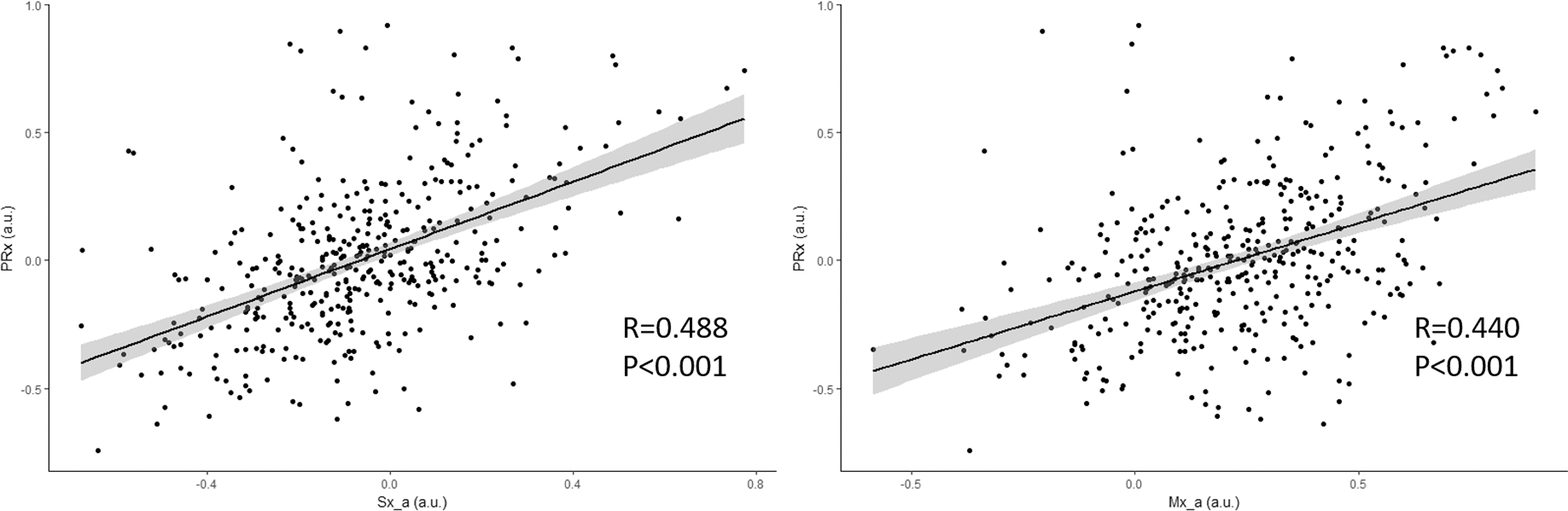
Linear relationship between pressure reactivity index (PRx; correlation between intracranial pressure and mean arterial pressure [MAP]), PRx versus systolic flow index (Sx_a; correlation between systolic flow velocity and MAP), and PRx versus mean flow index (Mx_a; correlation between mean velocity and MAP)—grand mean population data. a.u., arbitrary units; R, Pearson correlation coefficient.

ARIMA Modeling of PRx—patient example

Ten patients, with the longest continuous recordings, were analyzed initially to determine the ARIMA structure of PRx. All patients were deemed to display stationary signals for PRx, as assessed by ACF correlograms, ADF testing, and auto.arima algorithmic testing. Thus, no differencing factor was used. Figure 2 displays a patient example of the ACF and PACF correlograms on the raw PRx data, indicating rapid decay of significant lags on the ACF (panel A) and PACF (panel B) correlograms, confirming stationarity (ADF test = −4.456, p = 0.01).

FIG. 2.

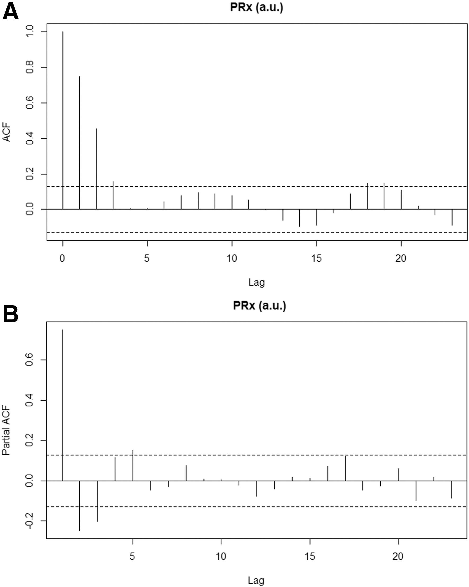
PRx (pressure reactivity index, correlation between intracranial pressure and mean arterial pressure) ACF (autocorrelation function) and PACF (partial autocorrelation function) correlograms—patient example. a.u., arbitrary units. Panel A, ACF correlogram; Panel B, PACF correlogram. Confidence intervals on correlograms (dotted lines) = ±(2/N^1/2), where N = sample size.

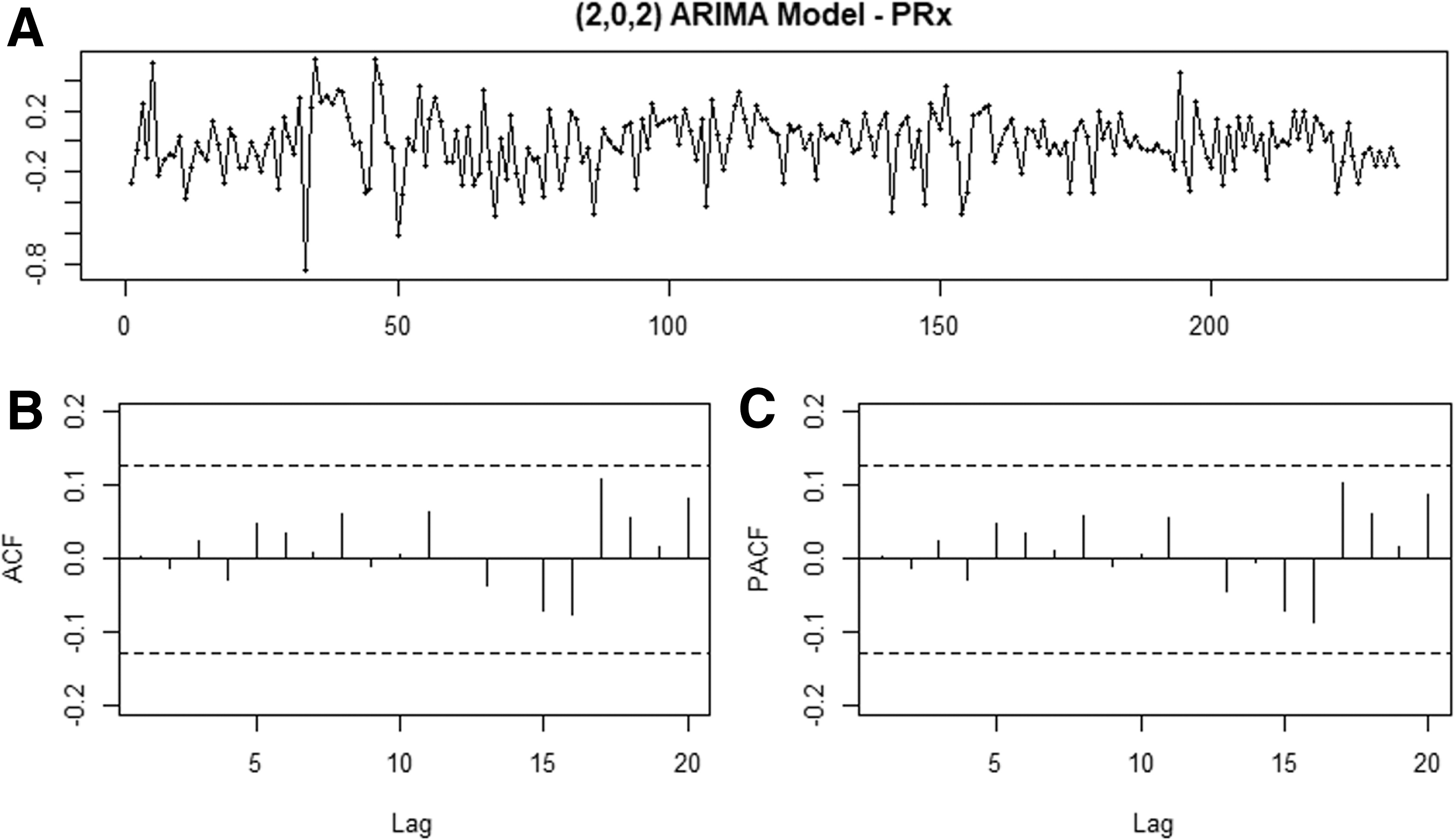
Running sequential iterative ARIMA models for PRx within the patient examples, we assessed the appropriate autoregressive order “p” and moving average order “q” for the PRx ARIMA model. We varied “p” from 0 to 3, and “q” from 0 to 3, assessing 16 separate ARIMA models for PRx. All models and their AICs and LL can be seen in Supplementary Appendix A; see online supplementary material at ftp.liebertpub.com. The most robust ARIMA structure for PRx, across the 10 patient examples, was deemed to be (2,0,2), with p = 2, d = 0, and q = 2. This model had the lowest AIC of −69.3 and among the highest LL of 39.65. Further, the residuals for this PRx ARIMA model appear random, with ACF/PACF correlograms indicating a lack of significant lags (Fig. 3). This ARIMA structure was confirmed with the auto.arima algorithm in R across all patient examples.

FIG. 3.

PRx (pressure reactivity index, correlation between intracranial pressure and mean arterial pressure) ARIMA (autoregressive integrative moving average) model (2,0,2) residual plot, ACF (autocorrelation function) and PACF (partial autocorrelation function) correlograms —patient example.

Confirmation of PRx ARIMA structure via sequential LME modeling

To confirm that the PRx (2,0,2) ARIMA model structure was adequate for the modeling across the entire dataset, we employed sequential LME models based on the fixed effects PRx ∼ Sx_a and random effects within the intercept (based on the patient), with varied embedded PRx ARIMA structures. We then ran the same 16 ARIMA model structures utilized within the patient examples, assessing the AIC, BIC, and LL of the LME models, with the goal of parsimony in the ARIMA structure. The data for AIC, BIC, and LL in each LME with the varied embedded PRx ARIMA error structures can be found in Supplementary Appendix B; see online supplementary material at ftp.liebertpub.com. The best model was again deemed to be that with a PRx ARIMA error structure of (2,0,2), with an AIC of −9797.294, BIC of −9735.699, and LL of 4906.647. The residual density for this model was normally distributed.

C. Model development and accuracy assessment

Our modeling of PRx using TCD-derived variables was conducted in two stages. First, we undertook modeling of PRx using the optimal autocorrelative structure that we identified in the previous section of results. We then compared measured (i.e., observed) and estimated PRx to determine how well our observed PRx values correlated with estimates from our top two models.

LME modeling of PRx using TCD indices

After confirming that ARIMA (2,0,2) error structure was adequate for continued LME modeling of PRx of the population, we fitted several different LME models to the whole data set, first varying the fixed effects model structure and then the random effects, as described within the Methods section. The AIC, BIC, and LL values for each LME model tested are presented in Table 1. The two best models, based on lowest AIC/BIC values, highest LL, and normally distributed residuals were: PRx ∼ Sx_a, and PRx ∼ Sx_a + Mx_a, with random effects (based on patient) introduced into both the independent variables and intercept. In addition, ANOVA testing indicated these two models were superior, with the multi-variable model (with Sx_a and Mx_a) being the most significant. The QQ plots and residual density plots for both models can be seen in Figure 4, indicating adequacy of the model. 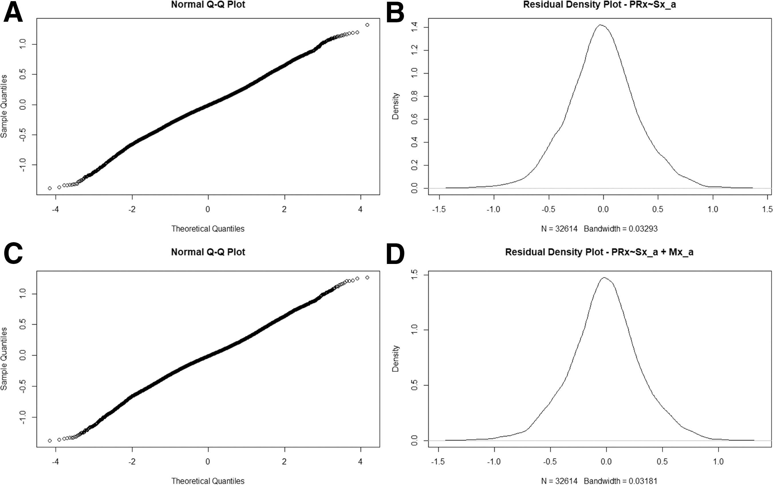The ACF and PACF plots of the residuals from each of these models can be found in Supplementary Appendix C (see online supplementary material at ftp.liebertpub.com), where an acceptable minimal number of lags is seen for each LME model in both the ACF and PACF plots of the residuals.

FIG. 4.

Quantile quantile (QQ) plot and residual density plot for two superior linear mixed effects (LME) models. Panel A = QQ plot for LME model PRx ∼ Sx_a (pressure reactivity index systolic flow index; Panel B = residual density plot for LME PRx ∼ Sx_a; Panel C = QQ plot for LME PRx ∼ Sx_a + Mx_a (mean flow index); Panel D = residual density plot for LME PRx ∼ Sx_a + Mx_a.

Table 1.

Linear Mixed Effects Models with Pressure Reactivity Index (2,0,2) Autoregressive Integrative Moving Average Structure—Entire Population

LME model		PRx ARIMA Structure
Fixed effects	Random effects	p	q	AIC	BIC	LL
PRx ∼ Sx_a	Intercept	2	2	−9797.294	−9735.699	4906.647
PRx ∼ Mx_a	Intercept	2	2	−8530.042	−8468.447	4273.021
PRx ∼ Dx_a	Intercept	2	2	−7865.311	−7803.716	3940.655
PRx ∼ Sx_a + Mx_a	Intercept	2	2	−9821.206	−9751.912	4919.603
PRx ∼ Sx_a + Dx_a	Intercept	2	2	−9804.395	−9735.101	4911.198
PRx ∼ Sx_a + Mx_a + Dx_a	Intercept	2	2	−9822.731	−9745.737	4921.365
PRx ∼ Sx_a	Intercept + Sx_a	2	2	-10806.43	-10729.44	5413.404
PRx ∼ Mx_a	Intercept + Mx_a	2	2	−9928.451	−9851.458	4974.226
PRx ∼ Dx_a	Intercept + Dx_a	2	2	−9239.414	−9162.420	4629.707
PRx ∼ Sx_a + Mx_a	Intercept + Sx_a + Mx_a	2	2	-11798.81	-11691.02	5913.404
PRx ∼ Sx_a + Dx_a	Intercept + Sx_a + Dx_a	2	2	FTC	FTC	FTC
PRx ∼ Sx_a + Mx_a + Dx_a	Intercept + Sx_a + Mx_a + Dx_a	2	2	FTC	FTC	FTC

LME, linear mixed effects model; PRx, pressure reactivity index (correlation between intracranial pressure [ICP] and mean arterial pressure [MAP]); ARIMA, auto-regressive integrative moving average; AIC, Akaike Information Criterion; BIC, Bayesian Information Criterion; LL, log likelihood; p, auto-regression parameter for ARIMA model; q, moving average parameter for ARIMA model; Sx_a, systolic flow index (correlation between transcranial Doppler (TCD)-based systolic flow velocity [FVs] and MAP); Mx_a; mean flow index (correlation between mean flow velocity [FVm] and MAP; Dx_a, diastolic flow index (correlation between TCD-based diastolic flow velocity (FVd) and MAP); FTC, “failure to converge” for the model.

Note: Bolded value represents the most appropriate ARIMA structure and LME model for the patient population tested, based on principle of parsimony, lowest AIC and BIC. There was no integrative parameter (i.e., “d” parameter) included within the ARIMA models, given stationarity testing during patient examples (see Supplementary Appendix A and Methods section of the article).

To evaluate further the impact of patient-by-patient variation on the LME model, we examined these models by removing the random components. Doing so produced inferior models, with larger AIC and BIC values. Further, comparing these population-wide generalized fixed effects models to the LME models via ANOVA, the LME models described above were statistically superior. All of the above for the entire population can be seen in Supplementary Appendix D; see online supplementary material at ftp.liebertpub.com.

Population-based estimation of PRx using Sx_a and Mx_a

Assessing the correlation between observed PRx and estimated PRx using the various models, we confirmed that the above mentioned superior LME models, with embedded PRx ARIMA structure of (2,0,2), displayed the best correlation between observed and estimated values. The model based on fixed effects of PRx ∼ Sx_a (with random effects in the coefficient and intercept based on patient) had a correlation of 0.794 (p < 0.0001, confidence interval [CI] = 0.788 to 0.799). The model based on fixed effects of PRx ∼ Sx_a + Mx_a (with the same random effects) displayed a correlation of 0.814 (p < 0.0001, CI = 0.809 to 0.819). All correlations between observed and estimated PRx for the LME models tested can be seen in Table 2.

Table 2.

Correlation Between Observed Pressure Reactivity Index and Linear Mixed Effects Model-Based Predicted Pressure Reactivity Index

LME model
Fixed effects	Random effects	Correlation between observed PRx and model predicted PRx
PRx ∼ Sx_a	Intercept	0.770
PRx ∼ Sx_a + Mx_a	Intercept	0.770
PRx ∼ Sx_a + Dx_a	Intercept	0.770
PRx ∼ Sx_a + Mx_a + Dx_a	Intercept	0.770
PRx ∼ Sx_a	Intercept + Sx_a	0.794
PRx ∼ Sx_a + Mx_a	Intercept + Sx_a + Mx_a	0.814
PRx ∼ Sx_a + Dx_a	Intercept + Sx_a + Dx_a	NA
PRx ∼ Sx_a + Mx_a + Dx_a	Intercept + Sx_a + Mx_a + Dx_a	NA

LME, linear mixed effects model; PRx = pressure reactivity index (correlation between intracranial pressure [ICP] and mean arterial pressure [MAP]); Sx_a = systolic flow index (correlation between transcranial Doppler [TCD]-based systolic flow velocity [FVs] and MAP); Mx_a; mean flow index (correlation between mean flow velocity [FVm] and MAP; Dx_a, diastolic flow velocity (correlation between TCD-based diastolic flow velocity (FVd) and MAP).

Note: bolded value represents the most appropriate autoregressive moving average structure and LME model for the patient population tested, based on principle of parsimony, lowest Akaike Information Criterion and Bayesian Information Criterion.

Figure 5 displays the linear relationship between observed and estimated grand mean PRx (i.e., average per patient) from the two optimal models: PRx ∼ Sx_a (Fig. 5A), and PRx ∼ Sx_a + Mx_a (Fig. 5B). Each model shows a strong linear correlation between observed PRx and model estimated PRx, with a slope almost equal to that of line “y = x” (dotted straight line in Fig. 5A and 5B).

FIG. 5.

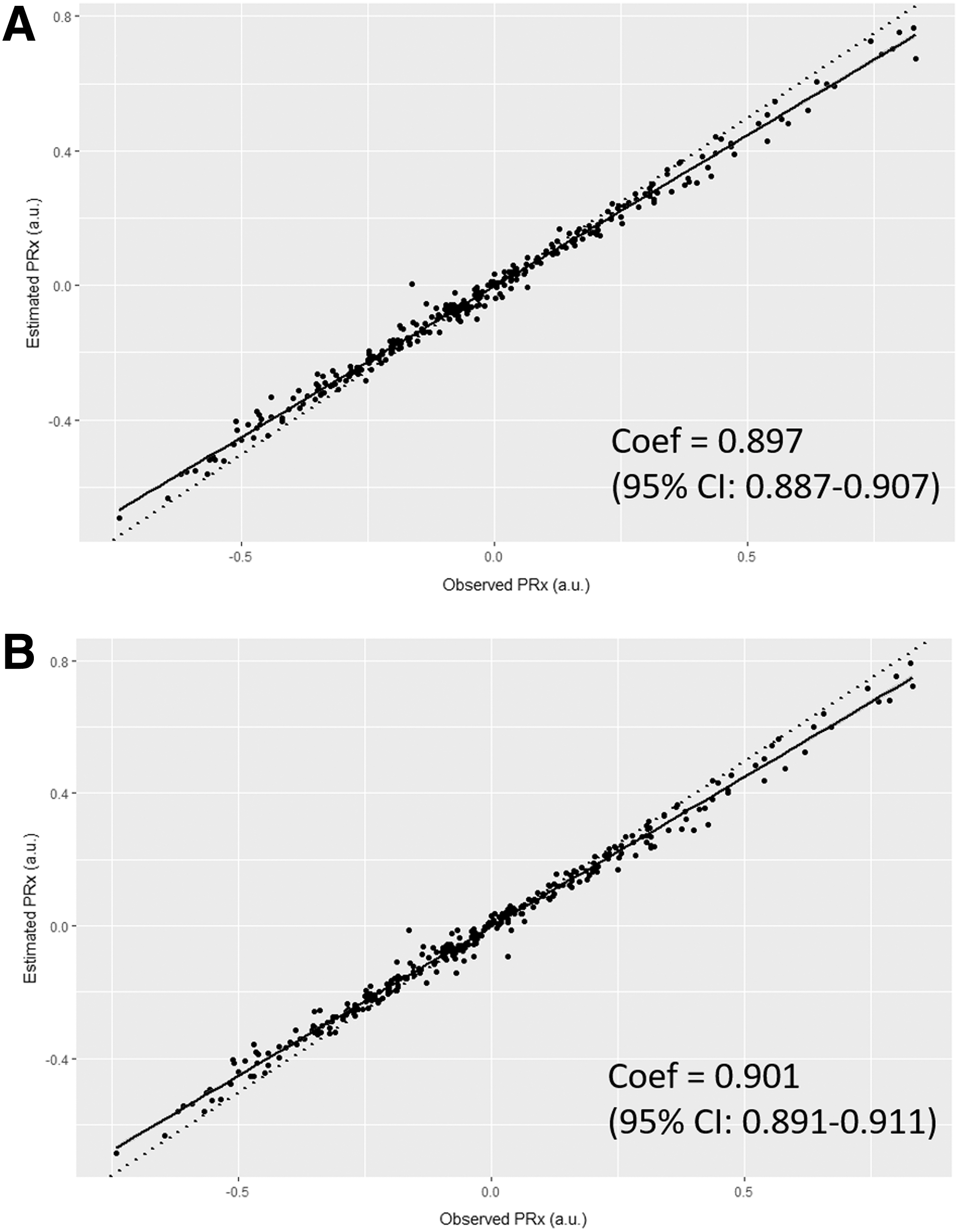
Linear regression between observed and estimated pressure reactivity index (PRx)—using estimated PRx (correlation between intracranial pressure and mean arterial pressure) from two best linear mixed effects (LME) models. Panel A: LME model—PRx ∼ Sx_a (systolic flow index; random effects with intercept and Sx_a); Panel B: LME model – PRx ∼ Sx_a + Mx_a (mean flow index; random effects with intercept, Sx_a and Mx_a); a.u.; arbitrary units; Coef, coefficients, from linear model between observed PRx and model estimated PRx. Dotted straight line represents the relationship “y = x”, for comparison to our two models.

Finally, Figure 6 displays the Bland-Altman plots for Fisher transformed grand mean data (i.e., average per patient), assessing the difference between observed and estimated PRx for each model (Fig. 6A and Fig. 6B). Both plots display good agreement between the observed and estimated PRx values for each model, within limits. Of note: the model estimates PRx well for values between +0.50 and −0.50 (approximately +0.46 and −0.46 in untransformed data, the common clinical range), where outside of that the agreement deteriorates.

FIG. 6.

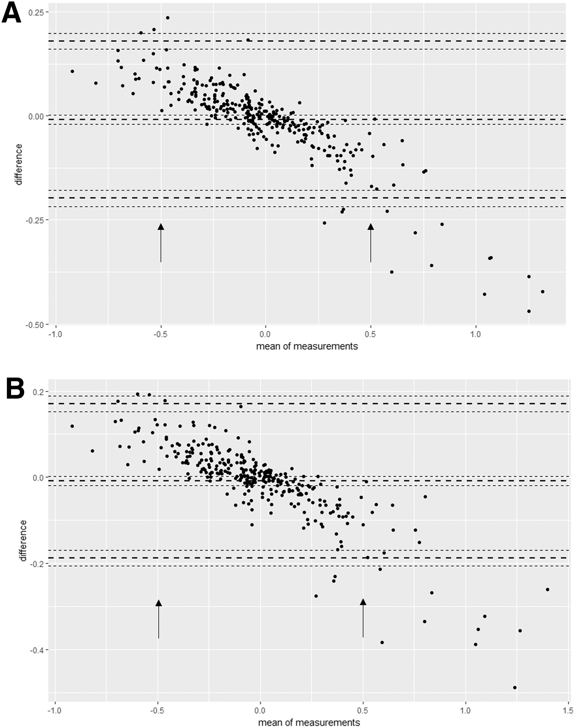
Bland-Altman plots—top two linear mixed effects (LME) models—observed versus estimated pressure reactivity index (PRx) (Fisher transformed [FT] grand mean data). Panel A: Bland-Altman plot comparing observed versus estimated PRx (correlation between intracranial pressure and mean arterial pressure) for LME model—PRx ∼ Sx_a (systolic flow index; random effects in intercept and Sx_a); Panel B: Bland-Altman plot comparing observed versus estimated PRx for LME model—PRx ∼ Sx_a + Mx_a (mean flow index; random effects in intercept, Sx_a and Mx_a). Horizontal bold dotted lines represent ±2 standard deviations in difference. Arrows denote margins of acceptable agreement between observed and estimated PRx, where outside of this range the agreement deteriorates.

Discussion

Through the application of LME modeling and accounting for the autocorrelative structure of PRx, via employing ARIMA modeling, we have been able to produce models that theoretically estimated PRx using noninvasive TCD autoregulation indices in patients with TBI. Further, we are able to estimate PRx with correlation between observed and estimated of ∼0.80, with acceptable agreement linear regression and Bland-Altman analysis. This is, to the authors' knowledge, the first attempt at applying time series and LME modeling of PRx and has laid the ground for further exploration of complex time series analysis of high frequency data in patients with TBI.

Some important points should be highlighted in this study. First, this is the first attempt at estimating an invasive autoregulation index, PRx, using noninvasive TCD measures, Sx_a and Mx_a. This is but a preliminary attempt at incorporating the complexities of time series analysis in the modeling of PRx. We have been able to produce theoretical models for estimating PRx; however, these are very preliminary and should be interpreted with caution. These results are promising for the future ability to estimate the “gold standard” PRx via noninvasive means. Further, we have displayed a strong relationship between noninvasive TCD-derived measures of cerebrovascular reactivity and the invasive derived gold-standard PRx, demonstrating that, in fact, PRx may be expressed in terms of these noninvasive measures.

This article identifies the strong link between two aspects of cerebral autoregulation, measures of cerebral blood flow (i.e., TCD-based CBFV) and measures of cerebral blood volume (i.e., ICP). Previous literature has displayed relatively poor correlation between these measures.^5,11 This article provides highly important evidence of a strong link between the two and offers explanation of that poor correlation. Second, the complexity of these models displays the difficulties in incorporating time series “real-time” analysis of high frequency physiological data from ICU monitoring. The application of ARIMA modeling is complex and labor intensive to find the most parsimonious model for our variable of interest, PRx. To ensure that we were applying the appropriate modeling, we employed various iterative techniques in both representative patient examples and a basic LME models in the entire dataset. Third, given the poor performance of the generalized fixed effects versions of our models, it is clear that there exists patient-by-patient variability that impacts the ability to model PRx, supporting the application of LME modeling. This cannot be ignored, as seen within our analysis. This was confirmed via AIC, BIC, LL, ANOVA, and correlation with observed PRx values—an important point for those wishing to employ generalized fixed effects models. Thus, the application of a generalized fixed effects model is limited, based on the results from our dataset.

Fourth, the Bland-Altman analysis provided further confirmation that our estimated PRx from the top two models were in good agreement with the observed PRx values in our patients. There is some bias evident within the Bland-Altman plots (i.e., the negative linear pattern seen), however, despite being within agreement throughout the normal range of PRx values typically encountered within the clinical setting (i.e., −0.5 to +0.5). This particular bias indicates that our models slightly overestimate PRx for positive values of observed PRx and underestimates PRx for negative values of observed PRx. Thus, our model is not perfect, but still closely estimates PRx within acceptable degrees of agreement. Finally, again this is preliminary work and these models should not be employed clinically at this time to estimate PRx using noninvasive TCD measures. Further analysis of these models and improvements need to occur before the reliability of their estimation can be determined.

Limitations

Some important limitations need to be highlighted. First, this is a retrospective analysis of a heterogeneous patient cohort. Thus, patient comorbidity, injury pattern/burden, and treatment heterogeneity may have impacted the recorded and archived high frequency signals utilized in the derivation of these autoregulation indices. Second, the ARIMA structure identified for PRx is only valid in this TBI patient sample. The (2,0,2) ARIMA structure may not apply to other cohorts of patients with TBI, or even other, perhaps longer recordings in the same patients. It is possible that the autoregressive order “p” as well as the moving average order “p” may be much higher in other cohorts. Further, the ARIMA structure of PRx based on different update periods, averaging process, and grouped averages (i.e., mean hourly values, mean daily values, etc.) has not been explored within this study.

Third, in our cohort, the signals appeared to fulfill the criteria for stationarity, based on various aspects of assessment. Thus, we did not apply a differencing order “d” in our ARIMA structure for PRx. We only assessed stationarity within the 10 longest patient recordings, however, generalizing the results of the stationarity assessment to the rest of the patient dataset. Thus, the short recordings not assessed could potentially have seasonality/trend that we did not account for. Further, it is possible that different populations of patients with TBI, different methods of acquiring PRx, and different averaging of the PRx data may introduce seasonality and trend to the data such that the signals become nonstationary. As well, our recordings were short; it may be that seasonality and trend were not appreciated in such short duration recordings, and longer recordings may display the need for a differencing order within the ARIMA structure for PRx. Much further evaluation of the autocorrelative structure for PRx and other high frequency physiologic variables in TBI is required.

Fourth, the inclusion of PRx ARIMA structure within the LME modeling adds significant complexity to the final models derived for the general population. This is a significant limitation to the application of these models broadly at this time. If further studies confirm and improve on the preliminary results displayed here, there is potential to automate this modeling and PRx estimation so that it is may become more accessible. Fifth, one could argue that the top two LME models displaying approximately 10 significant residual lags on the ACF plot indicate the model is not perfect. This is correct, and possibly a consequence of the short nature of the TCD recordings. With p values less than 1 × 10⁻¹⁶, however, we were confident that 10 residual lags would not inflate the p values so much that statistical significance could be questioned within the LME models. Hence, we were content with the results. Finally, the fact the generalized fixed effects models fail to display superiority to the LME models is a major limitation. This indicates that there is substantial patient-to-patient variability, limiting our ability to apply these models to other patients and datasets. Thus, we are unable to offer a general model for widespread use.

Future directions

Although the results of this current work are promising, they are, as mentioned, quite preliminary. Much further work is required to validate this work in other TBI populations, before its application in the noninvasive estimation of PRx via TCD. We plan to investigate other more detailed models, adjusting for patient demographic factors and injury pattern/burden. Further, it is unknown as to whether the addition of another noninvasive monitoring modality, such as near infrared spectroscopy, will provide any further estimative power within the models described in the article. Finally, the autocorrelative structure of PRx, among other physiologic variables monitoring in patients with TBI, requires much further extensive assessment. We plan to interrogate this structure in a larger TBI patient population, assessing how variations in PRx update frequency and grouped averaging impact this ARIMA structure. This would potentially provide valuable insight for future applications and integration of time series based PRx estimation and in TBI outcome modeling.

Future application of this type of time series modeling within neurotrauma and neurocritical care is wide reaching. We have just described the initial steps in modeling one aspect of cerebral physiology, cerebral autoregulation (i.e., PRx). These techniques are equally applicable to modeling ICP, MAP, or any other variable repeatably measured over time. Our models focused on simple univariate and “multi-variate” (i.e., two independent variables) LME modeling, while incorporating time series structure. This can be expanded to include many more pertinent variables, increasing accuracy in the modeling process. Further, we only described estimation of a physiological variable and compared that with the observed values at those specific time points.

Another logical step forward would be to apply these time series techniques to allow for forecasting (i.e., prediction) of PRx or other time dependent variables. If forecasting proves accurate, this would potentially enable us to predict upcoming physiologic events before they happened. An example would be based on the models described within this article, if they could be shown to accurately forecast future PRx values; then TCD could theoretically be utilized in the absence of invasive ICP monitoring to provide a forecasted noninvasive estimate of PRx. This, among other applications of physiologic forecasting, is, of course, some ways off currently, but not outside of the realm of possibility with appropriate time series-based modeling.

Conclusions

Through employing LME modeling and accounting for the autocorrelative structure of PRx with ARIMA modeling, one can theoretically estimate PRx using noninvasive TCD-based indices of cerebral autoregulation. We have described our first attempts at such modeling and PRx estimation; however, much more work is required to validate this complex work.

Footnotes

Acknowledgments

This work was made possible through salary support through the Cambridge Commonwealth Trust Scholarship, the Royal College of Surgeons of Canada – Harry S. Morton Travelling Fellowship in Surgery, the University of Manitoba Clinician Investigator Program, R. Samuel McLaughlin Research and Education Award, the Manitoba Medical Service Foundation, and the University of Manitoba Faculty of Medicine Dean's Fellowship Fund.

These studies were supported by National Institute for Healthcare Research (NIHR, UK) through the Acute Brain Injury and Repair theme of the Cambridge NIHR Biomedical Research Centre, an NIHR Senior Investigator Award to DKM. Authors were also supported by a European Union Framework Program 7 grant (CENTER-TBI; Grant Agreement No. 602150)

MC is supported by a grant of the Korea Health Technology R&D Project through the Korea Health Industry Development Institute (KHIDI), funded by the Ministry of Health & Welfare, Republic of Korea (grant number : HI17C1790).

JD is supported by a Woolf Fisher Scholarship (NZ).

Author Disclosure Statement

FAZ has received salary support for dedicated research time, during which this project was partially completed. Such salary support came from: the Cambridge Commonwealth Trust Scholarship, the Royal College of Surgeons of Canada – Harry S. Morton Travelling Fellowship in Surgery, the University of Manitoba Clinician Investigator Program, R. Samuel McLaughlin Research and Education Award, the Manitoba Medical Service Foundation, and the University of Manitoba - Faculty of Medicine Dean's Fellowship Fund. DKM has consultancy agreements and/or research collaborations with GlaxoSmithKline Ltd; Ornim Medical; Shire Medical Ltd; Calico Inc.; Pfizer Ltd; Pressura Ltd; Glide Pharma Ltd; and NeuroTraumaSciences LLC. MC and PS have financial interest in a part of licensing fee for ICM+ software (Cambridge Enterprise Ltd, UK). For the remaining authors, no competing financial interests exist.

References

Donnelly

, Budohoski

K.P.

, Smielewski

, and Czosnyka

(2016). Regulation of the cerebral circulation: bedside assessment and clinical implications. Crit. Care, 20, 129.

Czosnyka

, Miller

; and Participants in the International Multidisciplinary Consensus Conference on Multimodality Monitoring. (2014). Monitoring of cerebral autoregulation. Neurocrit. Care, 21, Suppl 2, S95–S102.

Zeiler

F.A.

, Donnelly

, Calviello

, Smielewski

, Menon

D.K.

, and Czosnyka

(2017). Pressure autoregulation measurement techniques in adult traumatic brain injury, Part II: a scoping review of continuous methods. J. Neurotrauma, 34, 3224–3237.

Le Roux

, Menon

D.K.

, Citerio

, Vespa

, Bader

M.K.

, Brophy

, Diringer

M.N.

, Stocchetti

, Videtta

, Armonda

, Badjatia

, Böesel

, Chesnut

, Chou

, Claassen

, Czosnyka

, De Georgia

, Figaji

, Fugate

, Helbok

, Horowitz

, Hutchinson

, Kumar

, McNett

, Miller

, Naidech

, Oddo

, Olson

, O'Phelan

, Provencio

J.J.

, Puppo

, Riker

, Robertson

, Schmidt

, and Taccone

; Neurocritical Care Society.; European Society of Intensive Care Medicine. (2014). Consensus summary statement of the International Multidisciplinary Consensus Conference on Multimodality Monitoring in Neurocritical Care: a statement for healthcare professionals from the Neurocritical Care Society and the European Society of Intensive Care Medicine. Neurocrit. Care, 21, Suppl 2, S1–S26.

Budohoski

K.P.

, Czosnyka

, de Riva

, Smielewski

, Pickard

J.D.

, Menon

D.K.

, Kirkpatrick

P.J.

, and Lavinio

(2012). The relationship between cerebral blood flow autoregulation and cerebrovascular pressure reactivity after traumatic brain injury. Neurosurgery, 71, 65–660.

Czosnyka

, Smielewski

, Kirkpatrick

, Laing

R.J.

, Menon

, and Pickard

J.D.

(1997). Continuous assessment of the cerebral vasomotor reactivity in head injury. Neurosurgery, 41, 11–17.

Sorrentino

, Diedler

, Kasprowicz

, Budohoski

K.P.

, Haubrich

, Smielewski

, Outtrim

J.G.

, Manktelow

, Hutchinson

P.J.

, Pickard

J.D.

, Menon

D.K.

, and Czosnyka

, (2012). Critical thresholds for cerebrovascular reactivity after traumatic brain injury. Neurocrit. Care, 16, 258–266.

Brady

K.M.

, Lee

J.K.

, Kibler

K.K.

, Easley

R.B.

, Koehler

R.C.

, and Shaffner

D.H.

(2008). Continuous measurement of autoregulation by spontaneous fluctuations in cerebral perfusion pressure: comparison of 3 methods. Stroke, 39, 2531–2537.

Lee

J.K.

, Kibler

K.K.

, Benni

P.B.

, Easley

R.B.

, Czosnyka

, Smielewski

, Koehler

R.C.

, Shaffner

D.H.

, and Brady

K.M.

(2009). Cerebrovascular reactivity measured by near-infrared spectroscopy. Stroke, 40, 1820–1826.

10.

Zweifel

, Castellani

, Czosnyka

, Helmy

, Manktelow

, Carrera

, Brady

K.M.

, Hutchinson

P.J.

, Menon

D.K.

, Pickard

J.D.

, and Smielewski

(2010). Noninvasive monitoring of cerebrovascular reactivity with near infrared spectroscopy in head-injured patients. J. Neurotrauma, 27, 1951–1958.

11.

Budohoski

K.P.

, Reinhard

, Aries

M.J.

, Czosnyka

, Smielewski

, Pickard

J.D.

, Kirkpatrick

P.J.

, and Czosnyka

(2012). Monitoring cerebral autoregulation after head injury. Which component of transcranial Doppler flow velocity is optimal?. Neurocrit. Care, 17, 211–218.

12.

Zeiler

F.A.

, Donnelly

, Menon

D.K.

, Smielewski

, Zweifel

, Brady

, and Czosnyka

(2017) Continuous autoregulatory indices derived from multi-modal monitoring: each one is not like the other. J. Neurotrauma, 34, 3070–3080.

13.

Zeiler

F.A.

, Cardim

, Donnelly

, Menon

D.K.

, Czosnyka

, and Smielewski

(2018). Transcranial Doppler systolic flow index and ICP-derived cerebrovascular reactivity indices in traumatic brain injury. J. Neurotrauma, 35, 314–322.

14.

Carney

, Totten

A.M.

, O'Reilly

, Ullman

J.S.

, Hawryluk

G.W.

, Bell

M.J.

, Bratton

S.L.

, Chesnut

, Harris

O.A.

, Kissoon

, Rubiano

A.M.

, Shutter

, Tasker

R.C.

, Vavilala

M.S.

, Wilberger

, Wright

D.W.

, and Ghajar

(2017). Guidelines for the Management of Severe Traumatic Brain Injury, Fourth Edition. Neurosurgery, 80, 6–15.

15.

Zeiler

F.A.

, Donnelly

, Cardim

, Menon

D.K.

, Smielewski

, and Czosnyka

(2017). ICP versus laser Doppler cerebrovascular reactivity indices to assess brain autoregulatory capacity. Neurocrit. Care. Epub ahead of print.

16.

Crawley

M.J.

(2013). Mixed Effects Models. In: The R Book, 2 ^nd ed. Wiley-Blackwell: Chichester, UK, pps. 681–710.

17.

Chatfield

, Tanner

, and Zidek

(Eds) (2004). The Analysis of Time Series, 6th ed. Chapman & Hall/CRC Press: Boca Raton, Florida, Chapters 1 to 9.

18.

Douc

, Moulines

, and Stoffer

D.S.

(2017). Nonlinear Time Series, 1st ed. Chapman & Hall/CRC Press: Boca Raton, Florida, Chapter 1.

Supplementary Material

Please find the following supplemental material available below.

For Open Access articles published under a Creative Commons License, all supplemental material carries the same license as the article it is associated with.

For non-Open Access articles published, all supplemental material carries a non-exclusive license, and permission requests for re-use of supplemental material or any part of supplemental material shall be sent directly to the copyright owner as specified in the copyright notice associated with the article.

0.00 MB

0.18 MB