A Probabilistic Framework for Peptide and Protein Quantification from Data-Dependent and Data-Independent LC-MS Proteomics Experiments

Abstract

A probability-based quantification framework is presented for the calculation of relative peptide and protein abundance in label-free and label-dependent LC-MS proteomics data. The results are accompanied by credible intervals and regulation probabilities. The algorithm takes into account data uncertainties via Poisson statistics modified by a noise contribution that is determined automatically during an initial normalization stage. Protein quantification relies on assignments of component peptides to the acquired data. These assignments are generally of variable reliability and may not be present across all of the experiments comprising an analysis. It is also possible for a peptide to be identified to more than one protein in a given mixture. For these reasons the algorithm accepts a prior probability of peptide assignment for each intensity measurement. The model is constructed in such a way that outliers of any type can be automatically reweighted. Two discrete normalization methods can be employed. The first method is based on a user-defined subset of peptides, while the second method relies on the presence of a dominant background of endogenous peptides for which the concentration is assumed to be unaffected. Normalization is performed using the same computational and statistical procedures employed by the main quantification algorithm. The performance of the algorithm will be illustrated on example data sets, and its utility demonstrated for typical proteomics applications. The quantification algorithm supports relative protein quantification based on precursor and product ion intensities acquired by means of data-dependent methods, originating from all common isotopically-labeled approaches, as well as label-free ion intensity-based data-independent methods.

Introduction

The aim of quantitative proteomics studies is to obtain information on the global changes in protein expression in two or more biological samples. The quantification of such changes is vital in understanding protein function, since subtle changes in expression level may well result in significant biological effects. The field is still rapidly growing and the techniques used for quantitative studies include 2D gel electrophoresis analysis, followed by quantification by means of optical density techniques and identification by mass spectrometry (MS) (Görg et al., 2004). Non-gel-based approaches utilize either stable isotope labeling strategies or label-free approaches in combination with separation and subsequent analysis by MS (Bantscheff et al., 2007). With increasing numbers of samples, the experimental design and statistical analysis of the results obtained becomes key. The use of statistics is common in the analysis of gene expression data, for which relatively large microarray data sets have to be evaluated, and for which univariate or single variable analysis methods do not suffice. In many respects, microarray data are analogous to quantitative proteomics data, and the same statistical techniques can often be applied. In other words, regardless of the (bio)analytical method applied to obtain the data, similar criteria can be applied to determine sample size, experimental design, and the number of required biological and technical replicates in relation to the desired power of the experiment (Horgan, 2007; Rocke, 2004).

As the complexity of datasets increases with the sophistication of the technology, it becomes correspondingly more important to adopt a coherent statistical methodology. To put it differently, the failings of other methods become more serious as technology advances. In fact, standard Bayesian probability calculus offers the only logically acceptable framework (Cox, 1946). Traditional orthodox statistical tests detract from coherent analysis, typically by producing different results when data constraints are applied in a different order (Jaynes, 2003). Such ad hoc testing procedures act to limit the quality and reliability of such inferences as are drawn.

Notwithstanding such criticisms, traditional statistical methods, such as the Student's t and ANOVA tests, are often used in conjunction with gel-based quantification techniques, and are considered to be established approaches (Gustafsson et al., 2004; Karp et al., 2007). More recently, q values have been introduced and used as an extension to false discovery rate calculations with their value assessed and used in quantitative 2D gel proteomics studies (Karp et al., 2007; Storey and Tibshirani, 2003). Multivariate statistical approaches are less frequently applied. The statistical methods mentioned above assume a normal distribution of the 2D gel data, which often requires normalization and/or transformation of the spot volumes (Gustafsson et al., 2004; Potra and Liu, 2006), and alignment of 2D gel images (Dowsey et al., 2008). Image alignment typically involves the identification of landmarks, warping of the images, and optionally creating a so-called composite master gel. This compensates for differences between gels caused by variations in migration, protein separation, stain artifacts, and stain saturation, which can otherwise complicate gel matching and quantification. More recently, a sample multiplexing technique has been developed for 2D gel analysis, which involves labeling of the sample prior to electrophoretic separation, to overcome limitations due to inter-gel variations (Unlü et al., 1997).

LC-MS-based proteomics quantification schemes also require normalization. However, in LC-MS experiments, a protein is typically represented by a greater number of features. Dependent on the labeling method of choice, a feature can be either a deconvoluted peptide precursor ion and its associated intensity, or product ions and their intensities. With inclusion of stable isotopes in the experimental design, normalization is typically conducted post-quantification. The complete data set is normally re-scaled by using either the mean or average value of all calculated ratio values (Li et al., 2007). Alternatively, summed intensities from all or selected components can be used. Components with ratios that lie outside a user-defined number of standard deviations from unity are typically considered to be significantly regulated (Li et al., 2003). Statistical outliers are removed with either Dixon's, Grubbs', or Rosner's tests (Aggarwal et al., 2005; Wong et al., 2008). With label-free LC-MS data, normalization can be conducted prior to the identification and quantification of the peptides and their originating parent proteins. The common nature of the LC-MS data, both within and across the complete data set, can be used to correct for systematic and/or sporadic changes (Kultima et al., 2009). This relies on the implicit assumption that changes in protein expression occur against a dominant background of proteins that do not change in their expression profile. Normalization can be conducted globally, where all LC-MS features are used simultaneously, or locally, where a subset of the features is used to calculate a normalization factor. Both approaches have been advocated and applied elsewhere (Callister et al., 2006; Tabata et al., 2007). Regardless of the type of normalization applied, time and m/z alignment (i.e., clustering of the detected features), has to be conducted first. A multitude of methods and algorithm types have been described, including correlation optimized warping (Prince and Marcotte, 2006), vectorized peaks (Hastings et al., 2002), (semi-) supervised alignment using non-linear regression methods (Fischer et al., 2006), hidden Markov models (Listgarten et al., 2007), statistical alignment (Wang et al., 2007), or more generic clustering methods (Lange et al., 2007; Mueller et al., 2007; Silva et al., 2005).

The above description gives an indication of the bewildering range of options available for analysis of protein expression data. Where a choice of tests is available, different practitioners may disagree about the selection and application for particular situations. For instance, missing data are sometimes dealt with by adding or imputing fictitious data (Little and Rubin, 2002), while the problem of uncertain assignment of observed features to predicted sequences may result in important data being discarded prematurely. This is an unsatisfactory situation, but it is by no means unique in data analysis (Dar et al., 1994). Fortunately, there exists a unique and consistent framework for reasoning with incomplete information that allows all sources of uncertainty to be combined using the standard rules of probability (Cox, 1946). In straightforward situations, the results often agree exactly with more traditional approaches, but awkward and universal features of large datasets, such as missing and outlying measurements, are accommodated automatically. In this article, we will illustrate that the presented framework can be applied to the quantitative analysis of proteomic data both at the protein and the peptide level. The robustness of the approach will be demonstrated by looking at protein quantification, including missing data, weak identifications, homologous peptides, and outlying measurements, with validated example data.

The transition from the qualitative characterization of complex proteomics samples to large-scale quantitative analysis by means of LC-MS has implications for the design of the overall experiment. In particular, the sample complexity and dynamic range, depth of the qualitative and quantitative proteome coverage desired, the required quantitative accuracy, and LC-MS instrumentation and acquisition settings, all impact the experimental strategy that is adopted. For example, the inherent dynamic range present in the sample compared with the dynamic range of the analytical approach chosen should determine whether sample fractionation at the protein or peptide level is required. The level of sample pre-fractionation performed will influence the selection of either a label-free or a label-dependent (stable isotope labeling) quantitative experiment (Patel et al., 2009; Wang et al., 2008a). The MS acquisition method settings are often not considered in quantitative experiments. However, the incorrect use of acquisition settings, such as the MS1 transmission window, precursor and product search tolerances, and instrument duty cycle settings, will all strongly impact the outcome of any type of proteomics experiment (Geromanos et al., 2009). Instrument characteristics such as ion saturation, either storage- (March and Todd, 2005; Williams and Cooks, 2005) or detection-related (Chemushevich et al., 2001), and how they can affect quantification are often not appreciated. The comprehensive statistical analysis of qualitative search results (Choi and Nesvizhskii, 2008; Fenyö and Beavis, 2003; Keller et al., 2002; Qian et al., 2005; Reiter et al., 2009), and that of quantitative LC-MS data (Listgarten et al., 2007; Smit et al., 2008), are attracting more attention with the realization that search algorithms were not designed with current sample complexity in mind. The interplay of these parameters and how they might be addressed are discussed within the context of the presented probabilistic quantification framework.

Materials and Methods

Sample preparation and tryptic digestion conditions

Cytosolic E. coli proteins differentially spiked with a standard protein mixture

An aliquot of 250 μL of 0.5% aqueous formic acid was added to 100 μg of a cytosolic E. coli tryptic digest standard. Tryptic digest stock solutions containing alcohol dehydrogenase, phosphorylase B, albumin, and enolase (Waters Corporation, Milford, MA), were prepared in 0.1% aqueous formic acid and diluted to a concentration of 25 fmol/μL for solution A, and 25, 12.5, 200, and 50 fmol/μL, respectively, for solution B. Equal volumes of the E. coli digest and the standard proteins mixture were combined to yield a sample concentration of 0.2 μg/μL of E. coli digest, and protein concentration ratios for protein mixture solution A versus protein mixture solution B of 1:1, 2:1, 1:8, and 1:2, respectively.

Yeast mitochondrial proteins

Yeast strain GT197 was grown at 30°C on glycerol medium prior to subsequent purification and fractionation of the mitochondria as previously described (Chacinska et al., 2000). Total protein fractions for Western blot analysis were obtained using a standard NaOH-TCA precipitation method (Nandakumar et al., 2003). The mitochondrial fractions were resolubilized in 50 mM ammonium bicarbonate/0.1% RapiGest solution (Waters Corporation), reduced in the presence of 100 mM dithiothreitol (DTT) (Sigma-Aldrich, St. Louis, MO) at 60°C for 30 min, and alkylated in the dark in the presence of 200 mM iodoacetamide (IAA) (Sigma-Aldrich) at room temperature for 30 min. Proteolytic digestion was initiated by adding sequence-grade modified trypsin (1:50 w/w) (Promega, Madison, WI), and incubated overnight at 37°C. Breakdown of acid-labile RapiGest was achieved in the presence of 4 μL of an aqueous 12 M HCl solution at 37°C for 15 min. The tryptic peptide solutions were centrifuged at 13,000 rpm for 10 min and the supernatant collected. Prior to LC-MS analyses, the tryptic peptide yeast solutions were diluted with aqueous 0.1% formic acid solution (Sigma-Aldrich) to provide adequate on-column loads, typically 0.3 μg. The LC-MS analyses were performed using 2 μL of the final protein digest mixtures.

Streptomyces coelicolor proteins

Streptomyces coelicolor M145 was grown in surface cultures and processed for protein extraction at eight different developmental time points as previously described (Manteca et al., 2006). Protein quantification was performed using a Bradford assay with a bovine serum albumin standard (Sigma-Aldrich). Proteins, 50 μg per lane, were separated by SDS-PAGE using precast PAGEr 4–20% Tris-Glycine gels (Lonza, Rockland, ME), and stained with Coomassie brilliant blue G-250 (Sigma-Aldrich). Each lane was divided into six strips and each gel piece was cut, washed, and shrunk with acetonitrile. Next, the cysteine residues were reduced with DTT and alkylated with IAA, swelled with a 10 ng/μL trypsin (Promega), 50 mM triethylammonium bicarbonate digestion buffer, and incubated overnight at 37°C. The supernatants were post-digestion recovered and peptide extraction from the gel fragments was performed with 25 μL of 5% formic acid for 30 min, after which an equal volume of pure acetonitrile was added and the samples were incubated for an additional 30 min at room temperature. Extracts obtained from each gel strip were pooled and vacuum-dried. The peptides were labeled with iTRAQ 8-plex reagent according to the manufacturer's instructions (Applied Biosystems, Foster City, CA). After labeling for 2 h at room temperature, all peptides from the gel pieces were combined (6 samples in total with 8 iTRAQ tags/developmental time points per sample). The concentration of the organic solvent was reduced using a vacuum concentrator. Peptide desalting (Gobom et al., 1999) was performed using GELoader micropipette tips (Eppendorf, Hamburg, Germany), prepared with C18 Empore extraction disks (3M, St. Paul, MN), and Poros R3 material (Applied Biosystems).

LC-MS configuration

Nanoscale LC separation of tryptic peptides was performed with a nanoACQUITY system (Waters Corporation), equipped with a Symmetry C₁₈ 5 μm, 5 mm×300-μm pre-column, and an Atlantis C18 3 μm, 15 cm×75-μm analytical reversed phase column (Waters Corporation). The experiments with the four-protein mixture added to the E. coli protein digest, the mitochondrial yeast proteins, were conducted in trapping configuration mode, and the Streptomyces coelicolor M145 sample was analyzed in direct on-column loading injection mode. Generic reversed-phase gradient conditions were applied to all samples and are summarized in Supplementary Table S1 (see online supplementary material at http://www.liebertonline.com). The four-protein mixture was added to the E. coli protein digest, and the mitochondrial yeast proteins and the yeast cytosolic protein fractions samples were all analyzed in triplicate (i.e., three technical replicates), unless stated otherwise.

The precursor ion masses and associated fragment ion spectra of the non-labeled tryptic peptides and the iTRAQ-labeled peptides were mass measured with a hybrid quadrupole orthogonal acceleration time-of-flight Q-Tof Premier or Synapt MS mass spectrometer (Waters Corporation, Manchester, U.K.), directly coupled to the chromatographic system. The time-of-flight analyzer of the mass spectrometer was externally calibrated, with the data post-acquisition lock mass corrected using the monoisotopic mass of the doubly charged precursor of [Glu¹]-fibrinopeptide B. The mass spectrometer acquisition parameters are provided in Supplementary Table S1 (see online supplementary material at http://www.liebertonline.com).

Accurate mass-measured data for the protein standards added to the E. coli protein digest, the mitochondrial yeast protein sample, were collected in a data-independent mode of acquisition by alternating the energy applied to the collision cell between a low-energy and elevated-energy state, as described previously (Bateman et al., 2002; Geromanos et al., 2009). The alternate scanning method combines peptide MS and multiplexed, data-independent peptide fragmentation MS analysis, in a single LC-MS experiment for the quantitative and qualitative characterization of a peptide mixture. The iTRAQ fragmentation data were collected in a data-dependent mode of acquisition. The mass spectrometer acquisition parameters scanning method details of the various experiments are summarized in Supplementary Table S1 (see online supplementary material at http://www.liebertonline.com).

LC-MS and LC-MS/MS data analysis

All continuum LC-MS data were processed using ProteinLynx GlobalSERVER version 2.5.2 (Waters Corporation). The data-independent fragment ion spectra from the four-protein mixture differentially spiked into the E. coli protein sample, the mitochondrial yeast proteins, and the yeast cytosolic proteins samples, were database searched with ProteinLynx GlobalSERVER version 2.5.2 as well. Protein identifications were accepted with more than three fragment ions per peptide, seven fragment ions per protein, and more than two peptides per protein identified. The search criteria used for protein identification included automatic peptide and fragment ion tolerance settings (most commonly 10 and 25 ppm, respectively), 1 allowed missed cleavage, fixed carbamidomethyl-cysteine modification, and variable methionine oxidation. The four-protein mixture added to the E. coli sample was database queried against a Comprehensive Microbial Resource (http://cmr.jcvi.org) E. coli K12 database (1 Nov. 2007, 4403 entries) appended with the four spiked proteins and trypsin. The mitochondrial yeast data were searched against a Saccharomyces Genome Database (http://www.yeastgenome.org) S. cerevisiae database (16 Feb. 2009, 6717 entries). The fragment ion spectra of the iTRAQ-labeled peptides of Streptomyces coelicolor were database searched using MASCOT version 2.2 against an NCBI (http://www.ncbi.nlm.nih.gov) Streptomyces coelicolor taxonomy limited database (22 Jan. 2009, 8537 entries). Protein redundancy was cleared with dbtoolkit (Martens et al., 2005). The peptide mass and fragment ion search tolerances were 10 ppm and 0.025 Da, respectively. Trypsin cleavage was specified with a maximum of 2 missed cleavages. Methyl methane thiosulfonate-cysteine, iTRAQ on lysine, and peptide N-termini, were set as fixed modifications. Methionine oxidation was considered as a variable modification. In all instances, for both the data-dependent and the data-independent searches, a one-time randomized decoy version of the individual databases was appended to the original databases.

Probabilistic Peptide and Protein Quantification Model

The problem of measuring the variation in concentration of a protein or peptide across two or more experimental conditions is considered. Each condition is often represented by several replicate acquisitions. Furthermore, each acquisition is subject to systematic errors, such as injection volume errors, and non-systematic effects, such as counting statistics. Due to the complexity of the samples and low concentration of some components, the data may be incomplete, and it can include interferences, and thus the assignment of data to peptides or clusters can be uncertain.

A consistent way of expressing and combining all such sources of uncertainty is required. Acknowledgment that standard probability calculus affords the only consistent route is called the Bayesian standpoint. Formally, x represents the quantities that are to be determined, augmented by any other parameters required to model the experimental data, and D actual data. Bayes' theorem, which is simply the product law of probability, states \documentclass{aastex}\usepackage{amsbsy}\usepackage{amsfonts}\usepackage{amssymb}\usepackage{bm}\usepackage{mathrsfs}\usepackage{pifont}\usepackage{stmaryrd}\usepackage{textcomp}\usepackage{portland, xspace}\usepackage{amsmath, amsxtra}\pagestyle{empty}\DeclareMathSizes{10}{9}{7}{6}\begin{document}\begin{align*}\underbrace{{\rm Pr} (x )}_{\rm Prior} \underbrace{{\rm Pr} (D | x)}_{\rm Likelihood} = \underbrace{{\rm Pr} ( D)}_{\rm Evidence} \underbrace{{\rm Pr} (x | D)}_{\rm Posterior}\end{align*}\end{document}

The likelihood function is the quantitative probability that a supposed x would produce the observed data, and it acts to modulate the prior possibilities into the posterior estimate. Meanwhile, the evidence is a number that offers quantitative assessment of whatever judgments and assignments led to the prior, should a user wish to compare alternative choices. The requirement of a prior, while logically necessary, puts the Bayesian standpoint in contrast to traditional approaches, which suppose that the issue can be evaded. For example, the Null Hypothesis Significance Test (NHST) attempts to use the likelihood alone to decide whether or not the data are consistent with some chosen null hypothesis x=x₀, to be retained or not as a result of the test. However, first, the NHST test is incoherent. Which data are to be used in the rejection of x₀? If only some, the analysis is inadequate because the other data are ignored. If all of a large dataset is used, there is very likely to be some minor unacknowledged and improperly modeled effect that damages the fit, leading to inappropriate rejection. Second, any continuous variable x almost certainly does differ from the hypothetical x_0, which, as a single point of the continuum, has measure zero. In other words, it is known at the outset that \documentclass{aastex}\usepackage{amsbsy}\usepackage{amsfonts}\usepackage{amssymb}\usepackage{bm}\usepackage{mathrsfs}\usepackage{pifont}\usepackage{stmaryrd}\usepackage{textcomp}\usepackage{portland, xspace}\usepackage{amsmath, amsxtra}\pagestyle{empty}\DeclareMathSizes{10}{9}{7}{6}\begin{document}$$x \neq x_0$$\end{document} with 99.999-recurring percent certainty, almost regardless of the data. Hence, the null hypothesis deserves no privileged status in parameter estimation. Similar criticisms can be made of other traditional procedures. For example, likelihood-based p values fail when the data produce unlikely but not impossible outliers (Jaynes, 2003). Methods that admit elementary counter-examples cannot be recommended, and we proceed with the Bayesian analysis that modern computing power makes feasible.

Peptide quantification

In peptide quantification it is assumed that model ion arrival rates are proportional to the peptide concentration in the injected sample. As an example, the situation in which data (ion counts) for a peptide are collected for two conditions with three replicate acquisitions for each condition is described. The assignments of the data to the peptide are initially not certain, so each has been assigned a reliability p (probability of being “good”) of 0.8. This assignment reflects the typical reliability of such information, and illustrates the sort of choice that often must be made when setting prior probabilities. There is no claim that such assignments are in any sense “true.” Rather, the choice is deemed reasonable, with substantially different settings being, in the authors' opinion, either implausibly strong or implausibly weak. The data are summarized in Table 1.

Table 1.

A Single Peptide in Two Different Conditions, Each of Which is Measured in Three Replicates

	Condition i=A		Condition i=B
Replicate	Counts D_Ak	Reliability P_Ak	Counts D_Bk	Reliability P_Bk
k=1	80	0.8	160	0.8
k=2	80	0.8	160	0.8
k=3	40	0.8	160	0.8

All of the data are assigned a reliability of 0.8.

In order to infer the peptide concentration ratio, a prior probability distribution Pr(y) for the peptide concentration y is specified. Here an exponential distribution is chosen \documentclass{aastex}\usepackage{amsbsy}\usepackage{amsfonts}\usepackage{amssymb}\usepackage{bm}\usepackage{mathrsfs}\usepackage{pifont}\usepackage{stmaryrd}\usepackage{textcomp}\usepackage{portland, xspace}\usepackage{amsmath, amsxtra}\pagestyle{empty}\DeclareMathSizes{10}{9}{7}{6}\begin{document}\begin{align*} {\rm Pr (y)} = \frac {e^{- y/\Lambda}}{\Lambda} \end{align*}\end{document}

where Λ is a hyper-parameter that may be interpreted as the scale of the intensities that are measured. Also, the probabilities of the different configurations of data which may be relevant to the peptide have to be considered, which are calculated from the reliabilities. In a particular configuration, each datum is either good (ON) or bad (OFF). In this case, there are 24 distinct configurations, whose multiplicities sum to 2⁶=64. The likelihood is \documentclass{aastex}\usepackage{amsbsy}\usepackage{amsfonts}\usepackage{amssymb}\usepackage{bm}\usepackage{mathrsfs}\usepackage{pifont}\usepackage{stmaryrd}\usepackage{textcomp}\usepackage{portland, xspace}\usepackage{amsmath, amsxtra}\pagestyle{empty}\DeclareMathSizes{10}{9}{7}{6}\begin{document}\begin{align*} &{\rm Pr}(\textbf{D}| y_A , y_B , S_{A1} , S_{A2} , S_{A3} , S_{B1} , S_{B2} , S_{B3}) \\& \qquad = \left[ \prod_{S_{ik} \in ON} \frac {e^{- y_{i}}y_i^{D_{ik}}} {D_{ik}!} \right] \left[\prod_{S_{ik} \in OFF} \frac {e^{- D_{ik}} / {\Lambda}} {\Lambda} \right] \end{align*}\end{document}

where S is the set of ON/OFF states in the current configuration, and D is the data in counts. The index i runs over the conditions A and B, while k runs over replicates 1–3. Note that the contribution to the likelihood from data that are ON is simply Poisson with mean y, whereas data that are OFF contributes via an exponential with mean Λ. The latter assignment reflects our ignorance of the predicted intensity of data unrelated to the peptide in question. Any data that have not been observed cannot appear in the likelihood; no interpolation or rejection of incomplete replicate sets is required. Moreover, this formulation can extract estimates of ratios and their uncertainties where there is only a single dataset of each condition and can be extended to describe any number of conditions and replicates.

The joint probability of all data for a single configuration is \documentclass{aastex}\usepackage{amsbsy}\usepackage{amsfonts}\usepackage{amssymb}\usepackage{bm}\usepackage{mathrsfs}\usepackage{pifont}\usepackage{stmaryrd}\usepackage{textcomp}\usepackage{portland, xspace}\usepackage{amsmath, amsxtra}\pagestyle{empty}\DeclareMathSizes{10}{9}{7}{6}\begin{document}\begin{align*} &{\rm Pr} (\textbf {D}, y_A , y_B , S_{A1} , S_{A2} , S_{A3}, S_{B1} , S_{B2} , S_{B3}) \\& \qquad = \frac {e^{-(y_{A} + y_{B})} / \Lambda} {\Lambda^2} \left[ \prod_{S_{ik} \in ON} \frac {P_{ik} e^{- y_{i}}y_i^{D_{ik}}} {D_{ik}!} \right] \left[ \prod_{S_{ik} \in OFF} \frac {({1 - p}_{ik})e^{-{D_{ik / \Lambda}}}} {\Lambda} \right] \end{align*}\end{document}

In this example, it is straightforward to marginalize over one of the y values to give a probability distribution for the ratio, y_B/y_A. This is plotted for the distinct configurations in Figure 1 with Λ equaling 113.3.

FIG. 1.

Probability versus log ratio for the 24 distinct configurations of switch ON/OFF states. Note that the scaling of the probability axes varies from plot to plot. The dominant configuration is 110–111 (log ratio ∼ log 2=0.693), shown in red. Its nearest subordinate configuration with a distinct maximum is 001-111 (log ratio ∼ log 4=1.386), shown in green.

The sum over all the configurations is shown in Figure 2. This is the total joint probability of the data and the log ratio.1 It should be noted that no attempt was made to reject outliers; unfavorable configurations are automatically down-weighted in terms of probability. The dominant configuration is 110-111 (i.e., s_A3 is OFF, all other switches are ON), as shown by the peak centered at about log 2=0.693. The subsidiary peak at around log 4=1.386 is mainly due to the 001-111 configuration.

FIG. 2.

The multiplicity-weighted sum of the configurations shown in Figure 1. The contribution from the dominant 110-111 configuration is shown in red, and that from the 001-111 configuration is shown in green.

Protein quantification

The treatment of proteins is very similar to that described for peptides. The data collected for a protein will generally consist of an incomplete set of measurements of ion counts for several peptides across the available conditions and replicates. A peptide is expected to have similar measured ion counts across technical replicates within a condition. On the other hand, different peptides may be produced with different efficiencies under enzymatic digestion, and they will ionize differently depending on their amino acid composition. The observation of different ion counts for different peptides belonging to the same protein is therefore to be expected, even within a condition. A further complication arises when distinct proteins in a mixture share one or more peptide sequence.

To capture this behavior, the model of the experimental situation is extended to include an extra degree of freedom z_j for each peptide j that captures its relative digestion and ionization characteristics. Ignoring any differences in digestion efficiency, the predicted ion count for peptide j in condition i becomes \documentclass{aastex}\usepackage{amsbsy}\usepackage{amsfonts}\usepackage{amssymb}\usepackage{bm}\usepackage{mathrsfs}\usepackage{pifont}\usepackage{stmaryrd}\usepackage{textcomp}\usepackage{portland, xspace}\usepackage{amsmath, amsxtra}\pagestyle{empty}\DeclareMathSizes{10}{9}{7}{6}\begin{document}\begin{align*}D_{ijk} = z_j \mathop\sum_{h \in H_{i}} y_{ih}\end{align*}\end{document}

where H_j is the set of proteins that produce peptide j, and y_ih is the concentration factor due to protein h in condition i. Rather than attempting to estimate the z_j, an exponential prior with a mean of unity is simply assigned to each one, allowing the y_ih to set the scale of the data through their dependence on Λ. The joint probability of the data D and parameters y, z, S is therefore \documentclass{aastex}\usepackage{amsbsy}\usepackage{amsfonts}\usepackage{amssymb}\usepackage{bm}\usepackage{mathrsfs}\usepackage{pifont}\usepackage{stmaryrd}\usepackage{textcomp}\usepackage{portland, xspace}\usepackage{amsmath, amsxtra}\pagestyle{empty}\DeclareMathSizes{10}{9}{7}{6}\begin{document}\begin{align*}Pr \textbf{(D , y , z , S )} = & \frac {1} {\Lambda^{N_{p}N_{c}}} e^{-} \frac {1} {\Lambda} \sum \nolimits_{i , h}{y_{ih}} \prod_{S_{ijk} \in {\rm ON}} \frac {p_{ijk}e^{- z_{j} \sum_{h \in H_{j}} y_{ih}}} {D_{ijk}!} \\ & \times \prod_{S_{ijk} \in { \rm OFF}} \frac {(1 - p_{ijk})e^{-D_{ijk}} / \Lambda} {\Lambda}\end{align*} \end{document}

Since we are not primarily interested in the z_j or the S_ijk_, we are free to integrate and sum over these “nuisance parameters” to obtain the marginal distribution \documentclass{aastex}\usepackage{amsbsy}\usepackage{amsfonts}\usepackage{amssymb}\usepackage{bm}\usepackage{mathrsfs}\usepackage{pifont}\usepackage{stmaryrd}\usepackage{textcomp}\usepackage{portland, xspace}\usepackage{amsmath, amsxtra}\pagestyle{empty}\DeclareMathSizes{10}{9}{7}{6}\begin{document}\begin{align*} {\rm Pr} (\textbf{D , y}) = \mathop \sum_{s} \int \ldots \int_{z + } dz {\rm Pr} ( \textbf{D , y , s , z})\end{align*}\end{document}

where the sum runs over all possible ON/OFF configurations and the integrals over the positive z orthant. In principle, this distribution contains all the information that is required to extract marginal posterior distributions for arbitrary functions of the protein concentration values y_ip, and in particular, the logarithm of the ratios y_mh/y_nh, between conditions m and n. Given these posterior distributions it is straightforward to extract means, standard deviations, credible intervals, regulation probabilities, and any other desired statistic.

Although this completes the formal definition of the method, in practice the direct summation over the different configurations of switch states used in the peptide quantification example quickly becomes unwieldy as the number of data to be considered increases. Instead, a Monte Carlo method is used to approximate the integral and direct summation. The use of two such techniques has been investigated for the problem of protein quantification, namely Gibbs sampling (Mackay, 2003), and nested sampling (Skilling, 2006). The suggested implementation of nested sampling uses a Gaussian approximation to the Poisson model likelihood \documentclass{aastex}\usepackage{amsbsy}\usepackage{amsfonts}\usepackage{amssymb}\usepackage{bm}\usepackage{mathrsfs}\usepackage{pifont}\usepackage{stmaryrd}\usepackage{textcomp}\usepackage{portland, xspace}\usepackage{amsmath, amsxtra}\pagestyle{empty}\DeclareMathSizes{10}{9}{7}{6}\begin{document}\begin{align*} \frac { e^ { - y } y^D } { D! } \approx \frac { e^ { - ( y - D ) ^2 / 2 } } { \sqrt { 2 \pi D } } \end{align*}\end{document}

While having negligible effect on the likelihood factors arising from ion counts other than the trivially small, which do not contribute to the inferences anyway, this approximation facilitates incorporation of non-Poisson uncertainties such as dead-time corrections.

Another practical issue arises due to small but noticeable systematic errors that occur during sample handling, enzymatic digestion of samples, and introduction of the samples into the LC-MS equipment. It is assumed that these effects result in ion counts that are systematically high or low in each replicate. It is beneficial to detect these variations and correct for them as part of the quantification process. This correction may use internal standards that are spiked into each sample at the same concentration or endogenous proteins whose concentrations are believed to be constant. Alternatively, normalization can be performed using the entire set of detected peptides as long as the biological perturbation being studied is not strong enough to affect more than a small fraction of the proteins identified. For similar reasons, random errors can be introduced, which result in variations in ion counts that exceed those expected from counting statistics alone. In order to incorporate these extra sources of uncertainty into the probabilistic analysis, a noise level is determined during the normalization process. This noise level is used to soften the observed data before quantification.

Normalization can be considered as another quantification problem in which each replicate is treated as a separate condition. When normalization is performed using the entire set of peptides, those belonging to proteins that do change will tend to be switched off. During the exploration, a relative strength is accumulated for the standards in each replicate. These strengths are used to correct the remaining data before the quantification step.

Results

Peptide and protein quantification

Three replicates of each of the differentially-spiked E. coli samples were acquired by means of data-independent alternate scanning. The raw data, in this instance stemming from a data-independent, label-free experiment, were processed and searched as described earlier. The database search was performed for each of the six individual experiments, which produces a list of protein identifications with associated peptides. Each peptide was accompanied by a reliability value. As an example, Table 2 shows the peptides identified from glycogen phosphorylase B in each experiment.

Table 2.

Deconvoluted Ion Count Measurements for Peptides Assigned to Phosphorylase B

Peptide	Mass	Mixture 1			Mixture 2
APNDFNLK	918.468	43739	42464	41985	20091	21543	19503
AWEVTVK	832.4563	29437	27550	29141	15991	11757	14656
DFNVGGYIQAVLDR	1566.7916	2526	2285	1704	1682	1618	1685
DFYELEPHK	1177.553	11000	10108	10230	5859	5233	5004
DYYFALAHTVR	1355.6743	6337	5716	5549	4722	4908	4458
EIWGVEPSR	1072.5422	25501	24420	26086	13335	12666	11782
FAAYLER	869.4516	33584	30213	32675	16572	15370	15572
GLAGVENVTELK	1229.6736	8284	7701	7955	3975	3792	3633
GLAGVENVTELKK	1357.7686	13318	12326	12808	11910	6244	11204
GYNAQEYYDR	1278.5386	10872	10595	10216	4770	4233	4844
GYNAQEYYDRIPELR	1886.9032	5772	5758	4614	3057	3201	3096
HLQIIYEINQR	1426.7806	39351				1347	1164
ICGGWQMEEADDWLR	1865.7953	1981	1976	1381	1758	1328
IGEEYISDLDQLR	1550.7697	10577	11248	10458	5747	6750	5346
IGEEYISDLDQLRK	1678.8646	8905	8858	7912	6459	6431	5868
IHSEILK	839.499	3626	3094	3327	1803	1608
IPELR	627.3829	4770	4524	4888	2222	2345	2064
LDWDK	676.3306	7860	6646	7660	3097
LITAIGDVVNHDPVVGDR	1890.008	8033	7183	6298	5332	4987	5244
LLSYVDDEAFIR	1440.7369	30064	26245	22698	16924	16774	13860
LPAPDEK	769.409	5444	4335	5471	2340	2428	2128
LPAPDEKIP	979.5459	20379	18819	17429	6598		4244
MSLVEEGAVK	1062.55	13200	11632	4841	6511	9367	5619
MSLVEEGAVKR	1218.6516	2020	1477
NLAENISR	916.4847	40309	39880	40267	19964	20110	18368
NNVVNTMR	947.4727	23365	21028	23762	11274	11783	11180
QIIEQLSSGFFSPK	1580.8319	20407	20236	15710	14838	14984	13476
QPDLFK	747.4041					24115
TCAYTNHTVLPEALER	1873.8992	15122	12732	13599	8299	8251	7456
TIAQYAR	822.4468	27721	26241	26104	11819	12856	12124
TNFDAFPDK	1054.484	39584	37633	38000	19302	18431	17385
TNGITPR	758.4155	7819	7165	7770	3828	3752	3305
TVMIGGK	705.3964	8174	8377	8263	4366	3977	3179
VAAAFPGDVDR	1117.5637	53247	47673	50548	24598	10621	21715
VEDVDR	732.3527	2304	2891	2833
VFADYEEYVK	1262.5939	1522	38455	38539	19685	19783	17700
VHINPNSLFDVQVK	1609.8701	2351		1625
VIFLENYR	1053.5728	65456	59062	58394	32751	31455	29881
VIPAADLSEQISTAGTEASGTGNMK	2448.1924	12821	10191	8861		6842	5303
VLVDLER	843.4934	49124	46238	49288	25311	24852	23452
VLYPNDNFFEGK	1442.6951	52527	50504	47530	25135	24388	22653
VSALYK	680.3978	10652	10360	10399	5282	5386	4390
VSLAEK	646.377	6104	6438	6293
YEFGIFNQK	1145.5626	16759	15877	15711	9090	9181	7578
YGNPWEK	893.4152	15131	15552	13811		7087	7541

The counts reported have been normalized using ADH as an internal standard. Green shading indicates a peptide identification probability of 0.95 or above, yellow denotes 0.5–0.95, and red denotes a probability of less than 0.5 (not applicable in this instance). A blank space corresponds to a missing identification. The nominal phosphorylase B concentration ratio equals 2:1 for mixture 1 versus. mixture 2.

Quantification was performed twice, first using Gibbs sampling as implemented in the quantification software and described here, followed by nested sampling. The results for the digest standards are given in Table 3. No results are provided for alcohol dehydrogenase, as it was used as an internal standard. In the course of the Gibbs Monte Carlo exploration, the average settings of the switches s_ijk for each peptide in each replicate were also accumulated. These numbers are effectively updates of the reliabilities P_ijk after all the data have been taken into account, and they give a measure of how strongly each peptide contributes to the reported protein ratio. All of the reported ratios in Table 3 are within a few percent of their nominal values (0.5, 2.0, and 8.0, respectively). Moreover, these values are included in the reported 95% credible intervals. The Gibbs algorithm and the nested sampling algorithm give very similar results. This result is encouraging, because it is expected that nested sampling will be more powerful under some circumstances, for example in the exploration of multi-modal distributions, or where the evidence might be used to calibrate the noise level (Skilling, 2006).

Table 3.

Quantification Results Using Gibbs and Nested Sampling

Protein	Ratio R	Log ratio R	95% Credible interval	Pr (R>1)
Gibbs sampling
Rabbit phosphorylase B	0.48	−0.73	±0.02	0.0
Yeast enolase	1.90	0.64	±0.04	1.0
Bovine serum albumin	7.77	2.05	±0.03	1.0
Nested sampling
Rabbit phosphorylase B	0.48	−0.73	±0.02	0.0
Yeast enolase	1.90	0.64	±0.05	1.0
Bovine serum albumin	7.77	2.05	±0.02	1.0

The nominal ratios are 0.5, 2.0, and 8.0. The credible interval applies to the log ratio.

The Gibbs sampling results for all proteins, including the digest standards, are summarized in Figure 3, which shows the reported ratios and credible intervals for all protein identification probabilities above 50%. The digest standards stand out clearly, and the E. coli proteins have ratios that are consistent with each other, but systematically only slightly higher than 1:1. This may be due to a small sample mixing error. Table 4 shows, as an example, the results for the three phosphorylase B peptides underlined in Table 2. The switch states illustrate how the algorithm deals with outlying and inconsistent measurements in real data. All technical replicates of both samples of the first peptide are consistent with the expected ratio. The second peptide is potentially problematic, in that two peptides of the second replicate are more consistent with a 1:1 ratio than the theoretical 2:1 ratio for phosphorylase B. The third peptide has conspicuous outliers in the third replicate of the first sample and the second replicate of the second sample.

FIG. 3.

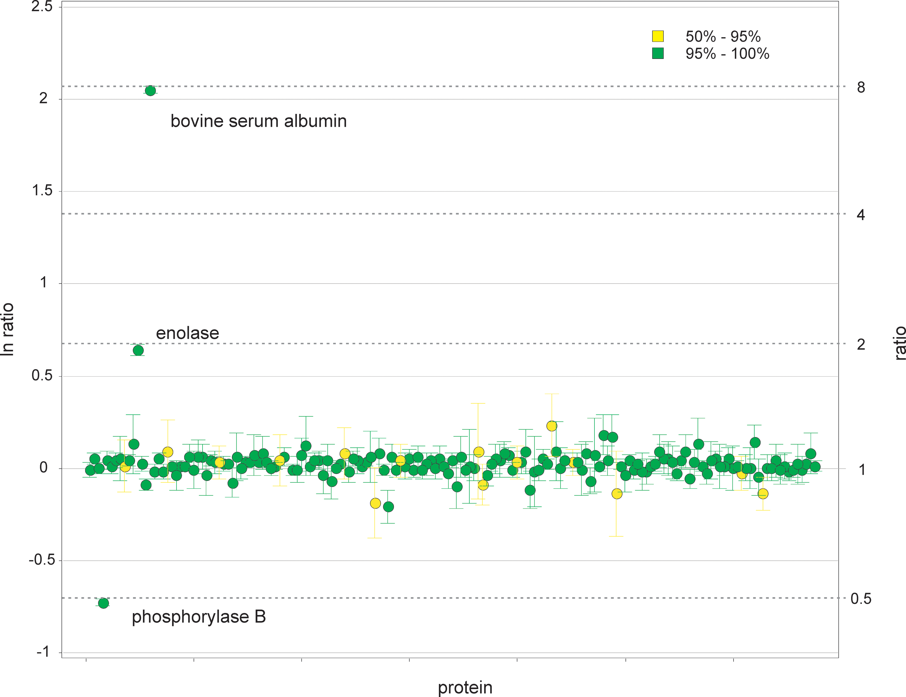
Quantification results for all proteins showing the 95% credible intervals. The colors denote identification probabilities. Nearly all of the E. coli proteins lie just below the line corresponding to a 1:1 ratio, indicating a slight differential E. coli amount between samples.

Table 4.

Average Switch States from Gibbs Sampling Showing the Importance of Each Individual Datum to the Algorithm

Peptide	Average switch states
APNDFNLK	1	1	1	1	1	1
GLAGVENVTELKK	1	1	0.99	0.02	1	0
MSLVEEGAVK	1	0.99	0	1	0.28	0.99

Green shading indicates a probability of 0.95 or above, yellow denotes 0.5–0.95, and red denotes a probability of less than 0.5.

In order to test simultaneous quantification of proteins sharing peptides, a simulated dataset was created. The relationships between the proteins involved are shown in Figure 4. The three proteins A, B, and C, produce three common peptides (PEPTIDEA, PEPTIDEC, and PEPTIDED). Each pair of proteins shares another two peptides, and each protein also produces two unique peptides. The simulated data relates to a two-condition experiment having three replicates in each condition. Each peptide is assigned a relative ionization factor, and the “true” expression ratios for the proteins between the two conditions are A (1:1), B (1:2), and C (4:1). Six data points have been corrupted intentionally, and three data points have been discarded. The input data including pseudo-random Poisson noise are shown in Table 5, and the results of the quantification analysis of the homologous proteins are given in Table 6. The expected relative abundances were within the inferred 95% credible intervals, consistent with the correct operation of the quantification framework for homologous proteins.

FIG. 4.

Network diagram for the quantification of homologous proteins.

Table 5.

Simulated Peptide Intensities for Homologous Proteins for Two Conditions Measured in Three Replicates

		Condition A			Condition B
Peptide sequence ¹	Proteins ²	Replicate 1	Replicate 2	Replicate 3	Replicate 1	Replicate 2	Replicate 3
PEPTIDEA	A B C	6925	1021	6828	6011	6026	5985
PEPTIDEC	A B C	14035	14084	14217	11927	11936	11991
PEPTIDED	A B C	21204	20999	20858	17926	18117	17910
PEPTIDEE	A B	12152	12062	12004	20162	1017	20172
PEPTIDEF	A B	15097	15159	14887	24825	24876	24970
PEPTIDEG	B C	12105	5979	5972	5015	4964	5013
PEPTIDEH	B C	12015	12069	11906	9992	9910	9988
PEPTIDEI	A C	14863	15072	14890	5917	5969	5929
PEPTIDEK	A	20165	—	19906	—	7926	8051
PEPTIDEL	A	5045	4975	4983	4986	5015	4948
PEPTIDEM	A	976	979	1037	969	1041	946
PEPTIDEN	B	1010	4043	4048	7923	7944	1009
PEPTIDEP	B	6034	6099	6197	12015	11983	12008
PEPTIDEQ	C	15975	16222	16169	4089	3938	4064
PEPTIDER	C	19770	973	19869	5018	5009	—

Peptides PEPTIDEA, PEPTIDEG, and PEPTIDEM are assigned a relative ionization value of 1, PEPTIDEC, PEPTIDEH, and PEPTIDEN a value of 2, PEPTIDED, PEPTIDEI, and PEPTIDEP a value of 3, PEPTIDEE, PEPTIDEK, and PEPTIDEQ a value of 4, and PEPTIDEF, PEPTIDEL, and PEPTIDER a value of 5.

The simulated relative protein abundance levels between conditions A and B for proteins A, B, and C are 1:1, 1:2, and 4:1, respectively.

All of the data are assigned a reliability of 0.9. Bold type indicates a simulated outlying measurement and — indicates missing data.

Table 6.

Quantification Results for Homologous Proteins

Protein	Ratio R	log ratio R	95% Credible interval
A	0.99	−0.01	± 0.04
B	1.93	0.66	± 0.04
C	0.25	−1.38	± 0.02

The nominal expected ratios are 1, 2, and 0.25, for proteins A, B, and C, respectively. The credible interval applies to the log ratio.

A difficulty arises when one or more proteins are identified using a subset of the peptides associated with another protein. For example protein A has associated peptides a, b, and c, protein B has associated peptides a, b, and c, and protein C is associated with peptides a and b. More generally, any unique peptides may be weak or unreliable. In this case, it is impossible to infer precise expression ratios for the proteins in question, but it would be possible to accumulate correlation statistics of the protein strengths during exploration. Proteins with strongly anti-correlated abundances could then be flagged for further investigation. For example, it might be appropriate to rerun quantification accumulating only ratios involving the sum of the strengths of the proteins in question.

Application examples

The first example involves the quantitative data-independent, label-free LC-MS analysis of the mitochondria of [PSI⁺] and [psi⁻] Saccharomyces cerevisiae strains (Chacinska et al., 2000). In this instance, no internal standard was added to the samples. As described above, for complex samples it is often possible to measure and correct for systematic errors taking into account slight differences in protein loading amounts without using an internal standard. The assumption is that changes in protein expression occur against a dominant background of proteins that are unaffected by the perturbation being studied. Supplementary Table S2 lists the normalization factors and associated uncertainties for each of the six experiments (see online supplementary material at http://www.liebertonline.com). The results suggest good technical replication, relatively small errors, and an estimated average ratio between the two conditions of interest of approximately 2.5. The latter is either indicative of different initial column loads, or as was the case in this example, significant variation in the studied sample types.

To illustrate the effect of auto-normalization, the monoisotopic doubly-charged precursor mass for tryptic fragment T11 identified for cytochrome c oxidase subunit 2 (Cox2) was extracted for one of the technical replicates of the [PSI⁺] and [psi⁻] samples. The ratio between the integrated areas of the chromatographic peaks shown in Supplementary Figure S1 is 0.159 (see online supplementary material at http://www.liebertonline.com). The quantification algorithm reported a ratio of 0.42 for Cox2, considering all technical replicates and identified peptides. Using the information provided in Supplementary Table S2, this reported normalized regulation factor can be converted to an un-normalized value of 0.161, which is in good agreement with the observed value in terms of raw peptide signal intensities (see online supplementary material at http://www.liebertonline.com).

The quantitative protein results were compared with the results obtained by Western blotting. In addition to Cox2, three other proteins were monitored, namely prohibitin-1 (PHB1), PROHIBITIN-2 (PHB2), and malate dehydrogenase (MDH1). A comparison of the results in terms of relative amounts is summarized in Supplementary Table S3 (see online supplementary material at http://www.liebertonline.com). Generally, the relative quantification results obtained by means of label-free LC-MS and Western blotting correlated well. Despite the modest observed relative expression of the Cox2, PHB1, and PHB2, the quantification algorithm gave consistent relative quantification values, supported by the reported upregulation probabilities. For Cox2 and PHB1, an upregulation probability of 0.00 was reported, and that of PHB2 was 0.02, illustrating in all instances a regulation probability greater than 95%. A more detailed description of the proteins identified and quantified in this study is presented elsewhere (Sikora et al., 2009), as well as the application of the quantification algorithm to other quantitative label-free nanoscale LC-MS applications (Chambery et al., 2009a, 2009b; Huang et al., 2007; Wang et al., 2008b; Xu et al., 2008).

The quantification framework described here is not restricted to quantitative label-free applications. Isotopically- and isobarically-labeled mass spectrometric data can also be analyzed under the assumptions that peptide or fragment intensities are provided for each peptide in each replicate. Examples of labeled techniques include iTRAQ, TMT, ¹⁸O, ICAT, and SILAC labeling (Gygi et al., 1999; Heller et al., 2003; Ong et al., 2002; Ross et al., 2004; Thompson et al., 2003). To illustrate the latter, iTRAQ relative quantification is demonstrated for the analysis of differences in the proteome of Streptomyces coelicolor during bacterial differentiation. Here, the quantification is based on product ion intensities in a multiplexed fashion. In other words, the samples are pooled and analyzed within a single experiment, whereas the previous label-free examples utilized precursor ion intensities from separate experiments. Figure 5 illustrates the MS/MS spectrum of one of the identified peptides, LLDEGQAGENVGLLLR, from an eight-plex experiment with samples obtained at different developmental stages. Shown inset is the product ion m/z region of interest that is utilized to estimate the ratio of the peptides. For this particular feature, the 113:114 peak-to-peak height ratio can easily be estimated and equals approximately 1.4.

FIG. 5.

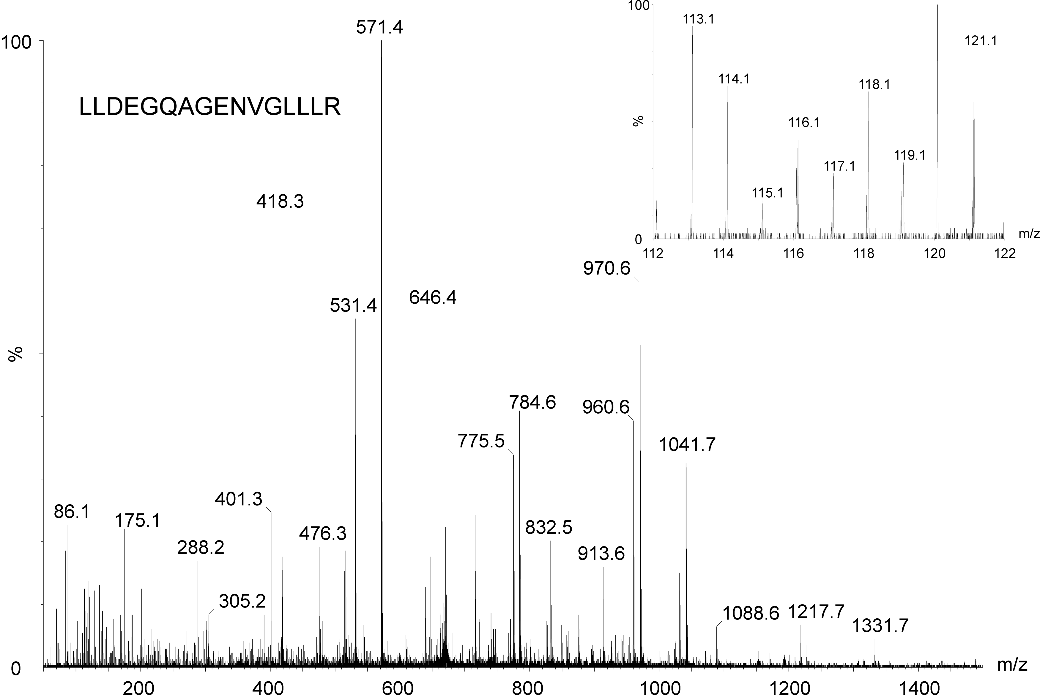
Qualitative and quantitative identification of LLDEGQAGENVGLLLR by means of iTRAQ isotopic labeling. The inset shows the reporter ion region of interest for quantitative analysis.

In this example, the data are reasonably consistent given the observed reporter ion intensities across peptides, as can be expected for iTRAQ data. Considering the 11 non-redundant identified peptides (12 in total) to the protein of interest, elongation factor, the calculated 113:114 reporter ion ratio equals 1.31 (0.27±0.24 for the log ratio), with a probability of upregulation of 1.00. The reported uncertainty is relatively large due to interference (i.e., background and chemical noise), which demonstrates one of the challenges one faces when employing fragment ions in LC-MS/MS-based quantification schemes. Manual inspection of the reporter ion intensities of the non-redundant peptides, excluding statistical outliers, gave a 113:114 ratio of 1.30. This value is plausibly close to the ratio calculated by the algorithm, which addressed the outlier data automatically.

A methodological replicate was labeled with two iTRAQ tags and processed as an internal control as a further test of the quantification algorithm. As expected for a technical replicate, the inferred logarithm of the reporter ion ratios for the majority of the proteins were close to zero, as illustrated by the red dots in Supplementary Figure S2, indicating no variation (see online supplementary material at http://www.liebertonline.com). The 95% credible region excluded a log ratio of zero for less than 6% of quantified proteins. The median protein log ratio was −0.04±0.39 (95% interquartile range). Supplementary Figure S2 also demonstrates the increased quantification variability that might be expected for proteins identified using lower-scoring peptides, and/or a reduced number of peptides, that can be utilized for quantification. In the case of the analysis of the reporter ion ratios by the algorithm for the same proteins between samples of different developmental stages, the calculated variation is in general greater than for the technical replicates, as illustrated by the grey background dots in Supplementary Figure S2 (see online supplementary material at http://www.liebertonline.com). Moreover, the relative protein abundance values in the Streptomyces coelicolor developmental phases analyzed have clear biological meaning, which is presented elsewhere in more detail (Manteca et al., 2010).

Discussion

With the analyses of complex biological samples, a number of aspects have to be acknowledged prior to providing a quantitative result. One of the initial considerations deals with the identification of redundant, non-proteotypic peptides. From a qualitative perspective there is a positive side effect, since the precursor and product ion intensities are cumulative, and the probability of identifying the peptide increases. However, these intensities must be handled carefully in quantitative analyses. High-quality proteotypic identifications can assist in the accurate quantification of isoforms and homologues. A second consideration is the chimeric nature of the data generated from a complex biological matrix. The presence of multiple precursors within the collision cell during an MS/MS acquisition can have a negative effect on both the qualitative and quantitative aspects of the results (Hoopmann et al., 2007; Luethy et al., 2008). These problems are exacerbated in instances in which the data is acquired on an instrument with relatively low resolving power (Cox et al., 2008; Mann and Kelleher, 2008). Qualitatively, lower MS/MS resolution allows for productions of similar mass originating from different precursors to overlap, creating a false impression of sensitivity. Additionally, product ions of dissimilar mass, originating for example from overlapping isotopic distributions, will occupy adjacent mass bins, providing a false sense of selectivity. Quantitatively, lower resolving power results in a precursor ion intensity value that is the sum of all of the co-eluting chimeric species. In addition to adding error in label-free quantitative experiments, chimericy/co-fragmentation is also problematic in labeled applications such as iTRAQ (Ross et al., 2004), or TMT labeling (Thompson et al., 2003). Here the presence of multiple precursors within the gas cell results in summed reporter ion intensities, analogous to the issues regarding isoforms and homologues described above. These and other challenges faced with reporter ion intensity–based quantification methods are discussed by others in greater detail (Ow et al., 2009). With the described probabilistic model, and highly selective and accurate data, these effects can be both acknowledged and addressed.

Other issues that have to be considered in quantitative isotope-labeled data-dependent LC-MS/MS approaches are the previously mentioned inherent increase in chimericy, and the decrease in dynamic range, that are evident when multiple biological samples are analyzed together (Bantscheff et al., 2007). In this instance, increased chimericy stems from the increased mass spectral complexity that occurs when the detected labeled/non-labeled peptides (both precursor and fragment ions) co-elute. With increased multiplexing (i.e., an increased number of combined biological samples), chimericy increases and challenges qualitative identification, as well the ensuing quantification. This is especially severe with lower-intensity ions, close to the detection limit of the mass spectrometer. The combined analysis of biological samples also decreases the effective sample dynamic range that can be measured, since the amount of sample that can be loaded onto the chromatographic system is directly proportional to the amount of available stationary phase. With a smaller amount of protein digest loaded per condition, both the sequence coverage and the opportunity for identifying proteotypic, sequence-unique information is reduced. As a direct result, the number of quantifiable peptides falls, increasing uncertainty in the result (Cui et al., 2009; Van et al., 2008). Alternatively, consistency of peptide identifications across biological and technical replicates might be limited (Ting et al., 2009), despite the application of stringent search criteria.

Conclusions

The presented Bayesian framework for the quantification of label-free and label-dependent LC-MS data provides a robust approach for expressing relative protein and peptide amounts. Missing data and uncertainties in assignments and measurements are easily accommodated. Outliers of any type and homologous peptides can be dealt with automatically, making the quantification algorithm suitable for a wide range of quantitative LC-MS applications. With label-free applications, any number of sample groups and replicates can be compared. In the instance of label-dependent applications, the number of comparisons is only limited by the number of possible labels.

For a well-characterized four-protein mixture in the presence of a complex biological background, the quantitative label-free LC-MS results were found to be consistent with the nominal changes in concentration, both within 2% and the 95% credible interval. The Gibbs algorithm and the newer nested sampling algorithm gave very similar results. This result is encouraging, because it is expected that nested sampling will be more powerful in some circumstances, for example, in the exploration of multi-modal distributions. Quantification of three homologous proteins was tested using a simulated dataset which included intentionally corrupted intensities and missing data. In all cases, the inferred log ratios were consistent with the nominal values.

Further verification of the performance of the quantification algorithm was achieved through comparison with results obtained by independent techniques. In the case of a label-free LC-MS application example, the obtained quantification results were consistent with those obtained using a bioanalytical assay. For a labeled application, iTRAQ in this particular example, the performance of the algorithm was assessed through the analysis of technical replicates. For over 94% of proteins the inferred log ratio was consistent with zero.

Footnotes

Acknowledgments

We kindly acknowledge Iain Campuzano, Phillip Young, Thérèse McKenna, Joanne B. Connolly, Scott J. Geromanos, Michael J. Nold, Ignatius J. Kass, LeRoy B. Martin, Martha Stapels, Craig A. Dorschel, Guo-Zhong Li, Jeffrey C. Silva, Dan Golick, Marc V. Gorenstein, and Timothy Riley for their valuable contributions throughout the development of this work.

Author Disclosure Statement

The authors declare that no conflicting financial interests exist.

1

Natural logarithms are used throughout. Log ratios make the symmetry between up and down regulation clear since they change sign if the labels on the two samples are exchanged. In addition, probability distributions for log ratios are often more symmetric than for the direct ratio. All error bars for log ratios define a 95% credible interval.

References

Aggarwal

, Choe

L.H.

, Lee

K.H.

2005. Quantitative analysis of protein expression using amine-specific isobaric tags in Escherichia coli cells expressing rhsA elements. Proteomics, 5:2297–2308.

Bantscheff

, Schirle

, Sweetman

, Rick

, Kuster

2007. Quantitative mass spectrometry in proteomics: a critical review. Anal Bioanal Chem, 389:1017–1031.

Bateman

R.H.

, Carruthers

, Hoyes

J.B.

et al. 2002. A novel precursor ion discovery method on a hybrid quadrupole orthogonal acceleration time-of-flight (Q-TOF) mass spectrometer for studying protein phosphorylation. J Am Soc Mass Spectrom, 13:792–803.

Callister

S.J.

, Barry

R.C.

, Adkins

J.N.

et al. 2006. Normalization approaches for removing systematic biases associated with mass spectrometry and label-free proteomics. J Proteome Res, 5:277–286.

Chacinska

, Boguta

, Krzewska

, Rospert

2000. Prion-dependent switching between respiratory competence and deficiency in the yeast nam9-1 mutant. Mol Cell Biol, 20:7220–7229.

Chambery

, Colucci-D'Amato

, Vissers

J.P.

, Scarpella

, Langridge

J.I.

, Parente

2009. Proteomic profiling of proliferating and differentiated neural mes-c-myc A1 cell line from mouse embryonic mesencephalon by LC-MS. J Proteome Res, 8:227–238.

Chambery

, Vissers

J.P.

, Langridge

J.I.

et al. 2009. Qualitative and quantitative proteomic profiling of cripto(-/-) embryonic stem cells by means of accurate mass LC-MS analysis. J Proteome Res, 8:1047–1058.

Chernushevichm

I.V.

, Loboda

A.V.

, Thomson

B.A.

2001. An introduction to quadrupole-time-of-flight mass spectrometry. J Mass Spectrom, 36:849–865.

Choi

, Nesvizhskii

A.I.

2008. False discovery rates and related statistical concepts in mass spectrometry-based proteomics. J Proteome Res, 7:47–50.

10.

Cox

, Hubner

N.C.

, Mann

2008. How much peptide sequence information is contained in ion trap tandem mass spectra? J Am Soc Mass Spectrom, 19:1813–1820.

11.

Cox

R.T.

1946. Probability, frequency and reasonable expectation. Am J Phys, 14:1–3.

12.

Cui

, Chen

, Lu

et al. 2009. Preliminary quantitative profile of differential protein expression between rat L6 myoblasts and myotubes by stable isotope labeling with amino acids in cell culture. Proteomics, 9:1274–1292.

13.

Dar

, Serlin

C.S.

, Omer

1994. Misuse of statistical tests in three decades of psychotherapy research. J Consult Clin Psychol, 62:75–82.

14.

Dowsey

A.W.

, Dunn

M.J.

, Yang

G.Z.

2008. Automated image alignment for 2D gel electrophoresis in a high-throughput proteomics pipeline. Bioinformatics, 24:950–957.

15.

Fenyö

, Beavis

R.C.

2003. A method for assessing the statistical significance of mass spectrometry-based protein identifications using general scoring schemes. Anal Chem, 75:768–774.

16.

Fischer

, Grossmann

, Roth

et al. 2006. Semi-supervised LC/MS alignment for differential proteomics. Bioinformatics, 22:132–140.

17.

Geromanos

S.J.

, Vissers

J.P.

, Silva

J.C.

et al. 2009. The detection, correlation and comparison of peptide precursor and product ions from data independent LC-MS with data dependent LC-MS/MS. Proteomics, 9:1683–1695.

18.

Gobom

, Nordhoff

, Mirgorodskaya

, Ekman

, Roepstorff

1999. Sample purification and preparation technique based on nano-scale reversed-phase columns for the sensitive analysis of complex peptide mixtures by matrix-assisted laser desorption/ionization mass spectrometry. J Mass Spectrom, 34:105–116.

19.

Görg

, Weiss

, Dunn

M.J.

2004. Current two-dimensional electrophoresis technology for proteomics. Proteomics, 4:3665–3685.

20.

Gustafsson

J.S.

, Ceasar

, Glasbey

C.A.

, Blomberg

, Rudemo

2004. Statistical exploration of variation in quantitative two-dimensional gel electrophoresis data. Proteomics, 4:3791–3799.

21.

Gygi

S.P.

, Rist

, Gerber

S.A.

, Turecek

, Gelb

M.H.

, Aebersold

1999. Quantitative analysis of complex protein mixtures using isotope-coded affinity tags. Nat Biotech, 17:994–999.

22.

Hastings

C.A.

, Norton

S.M.

, Roy

2002. New algorithms for processing and peak detection in liquid chromatography/mass spectrometry data. Rapid Commun Mass Spectrom, 16:462–467.

23.

Heller

, Mattou

, Menzel

, Yao

2003. Trypsin catalyzed ¹⁶O-to-¹⁸O exchange for comparative proteomics: tandem mass spectrometry comparison using MALDI-TOF, ESI-QTOF and ESI-ion trap mass spectrometers. J Am Soc Mass Spectrom, 14:704–718.

24.

Hoopmann

M.R.

, Finney

G.L.

, MacCoss

M.J.

2007. High-speed data reduction, feature detection and MS/MS spectrum quality assessment of shotgun proteomics data sets using high-resolution mass spectrometry. Anal Chem, 79:5620–5632.

25.

Horgan

G.W.

2007. Sample size and replication in 2D gel electrophoresis studies. J Proteome Res, 6:2884–2887.

26.

Huang

J.T.

, McKenna

, Hughes

, Leweke

F.M.

, Schwarz

, Bahn

2007. CSF biomarker discovery using label-free nano-LC-MS based proteomic profiling: technical aspects. J Sep Sci, 30:214–225.

27.

Karp

N.A.

, McCormick

P.S.

, Russel

M.R.

, Lilley

K.S.

2007. Experimental and statistical considerations to avoid false conclusions in proteomics studies using differential in-gel electrophoresis. Mol Cell Proteomics, 6:1354–1364.

28.

Keller

, Nesvizhskii

A.I.

, Kolker

, Aebersold

2002. Empirical statistical model to estimate the accuracy of peptide identifications made by MS/MS and database search. Anal Chem, 74:5383–5392.

29.

Kultima

, Nilsson

, Scholz

, Rossbach

U.L.

, Fälth

, Andrén

P.E.

2009. Development and evaluation of normalization methods for label-free relative quantification of endogenous peptides. Mol Cell Proteomics, 8:2285–2295.

30.

Jaynes

E.T.

2003. Principles and pathology of orthodox statistics. Probability Theory: The Logic of Science. Bretthorst

G.L.

Cambridge: Cambridge University Press.

31.

Lange

, Gröpl

, Schulz-Trieglaff

, Leinenbach

, Huber

, Reinert

2007. A geometric approach for the alignment of liquid chromatography-mass spectrometry data. Bioinformatics, 2007:i273–i281.

32.

K.W.

, Miller

, Klychnikov

et al. 2007. Quantitative proteomics and protein network analysis of hippocampal synapses of CaMKIIalpha mutant mice. J Proteome Res, 6:3127–3133.

33.

Listgarten

, Neal

R.M.

, Roweis

S.T.

, Wong

, Emili

2007. Difference detection in LC-MS data for protein biomarker discovery. Bioinformatics, 23:198–204.

34.

Little

R.J.A.

, Rubin

D.B.

2002. Statistical Analysis with Missing Data, 2nd. New York: John Wiley and Sons.

35.

X.J.

, Zhang

, Ranish

J.A.

, Aebersold

2003. Automated statistical analysis of protein abundance ratios from data generated by stable-isotope dilution and tandem mass spectrometry. Anal Chem, 75:6648–6657.

36.

Luethy

, Kessner

D.E.

, Katz

J.E.

et al. 2008. Precursor-ion mass re-estimation improves peptide identification on hybrid instruments. J Proteome Res, 7:4031–4039.

37.

Mackay

D.J.C.

2003. Information Theory, Inference and Learning Algorithms. Cambridge: Cambridge University Press.

38.

Mann

, Kelleher

N.L.

2008. Precision proteomics: The case for high resolution and high mass accuracy. PNAS, 105:18132–18138.

39.

Manteca

, Mäder

, Connolly

B.A.

, Sanchez

2006. A proteomic analysis of Streptomyces coelicolor programmed cell death. Proteomics, 6:6008–6022.

40.

Manteca

, Sanchez

, Jung

H.R.

, Schwämmle

, Jensen

O.N.

2010. Quantitative proteomic analysis of Streptomyces coelicolor development demonstrates the switch from primary to secondary metabolism associated with hyphae differentiation. Mol Cell Proteomics, 9:1423–1436.

41.

March

R.E.

, Todd

J.F.

2005. Quadrupole Ion Trap Mass Spectrometry, 2nd. New York: John Wiley and SonsChap. 5161.

42.

Martens

, Vandekerckhove

, Gevaert

2005. DBToolkit: processing protein databases for peptide-centric proteomics. Bioinformatics, 21:3584–3585.

43.

Mueller

L.N.

, Rinner

, Schmidt

et al. 2007. SuperHirn—a novel tool for high resolution LC-MS-based peptide/protein profiling. Proteomics, 7:3470–3480.

44.

Nandakumar

M.P.

, Shen

, Raman

, Marten

M.R.

2003. Solubilization of trichloroacetic acid (TCA) precipitated microbial proteins via NaOH for two-dimensional electrophoresis. J Proteome Res, 2:89–93.

45.

Ong

S.E.

, Blagoev

, Kratchmarova

et al. 2002. Stable isotope labeling by amino acids in cell culture, SILAC, as a simple and accurate approach to expression proteomics. Mol Cell Proteomics, 1:376–386.

46.

S.Y.

, Salim

, Noirel

, Evans

, Rehman

, Wright

P.C.

2009. iTRAQ underestimation in simple and complex mixtures: “The good, the bad and the ugly.” J Proteom Res, 8:5347–5355.

47.

Patel

V.J.

, Thalassinos

, Slade

et al. 2009. A comparison of labelling and label-free mass spectrometry-based proteomics approaches. J Proteome Res, 8:3752–3759.

48.

Potra

F.A.

, Liu

2006. Aligning families of two-dimensional gels by a combined multiresolution forward-inverse transformation approach. J Comput Biol, 3:1384–1395.

49.

Prince

J.T.

, Marcotte

E.M.

2006. Chromatographic alignment of ESI-LC-MS proteomics data sets by ordered bijective interpolated warping. Anal Chem, 78:6140–6152.

50.

Qian

W.J.

, Liu

, Monroe

M.E.

et al. 2005. Probability-based evaluation of peptide and protein identifications from tandem mass spectrometry and SEQUEST analysis: the human proteome. J Proteome Res, 4:53–62.

51.

Reiter

, Claassen

, Schrimpf

S.P.

et al. 2009. Protein identification false discovery rates for very large proteomics datasets generated by tandem mass spectrometry. Mol Cell Proteomics, 8:2405–2417.

52.

Rocke

D.M.

2004. Design and analysis of experiments with high throughput biological assay data. Semin Cell Dev Biol, 15:703–713.

53.

Ross

P.L.

, Huang

Y.N.

, Marchese

J.N.

et al. 2004. Multiplexed protein quantification in Saccharomyces cerevisiae using amine-reactive isobaric tagging reagents. Mol Cell Proteomics, 3:1154–1169.

54.

Sikora

, Kistowski

, Rubel

et al. 2009. Yeast prion [PSI+] lowers the levels of mitochondrial prohibitins. Biochim Biophys Acta, 1793:1703–1709.

55.

Silva

J.C.

, Denny

, Dorschel

C.A.

et al. 2005. Quantitative proteomic analysis by accurate mass retention time pairs. Anal Chem, 77:2187–2200.

56.

Skilling

2006. Nested sampling for general Bayesian computation. J Bayesian Analysis, 1:833–860.

57.

Smit

, Hoefsloot

H.C.J.

, Smilde

A.K.

2008. Statistical data processing in clinical proteomics. J Chromatogr B, 866:77–88.

58.

Storey

J.D.

, Tibshirani

2003. Statistical significance for genomewide studies. Proc Natl Acad Sci USA, 100:9440–9445.

59.

Tabata

, Sato

, Kuromitsu

, Oda

2007. Pseudo internal standard approach for label-free quantitative proteomics. Anal Chem, 79:8440–8445.

60.

Thompson

, Schäfer

, Kuhn

et al. 2003. Tandem Mass Tags: A novel quantification strategy for comparative analysis of complex protein mixtures by MS/MS. Anal Chem, 75:1895–1904.

61.

Unlü

, Morgan

M.E.

, Minden

J.S.

1997. Difference gel electrophoresis: a single gel method for detecting changes in protein extracts. Electrophoresis, 18:2071–2077.

62.

Ting

, Cowley

M.J.

, Hoon

S.L.

, Guilhaus

, Raftery

M.J.

, Cavicchioli

2009. Normalization and statistical analysis of quantitative proteomics data generated by metabolic labeling. Mol Cell Proteomics, 8:2227–2242.

63.

Van

P.T.

, Schmid

A.K.

, King

N.L.

et al. 2008. Halobacterium salinarum NRC-1 PeptideAtlas: toward strategies for targeted proteomics and improved proteome coverage. J Proteome Res, 7:3755–3764.

64.

Wang

, Ye

, Dong

et al. 2008a. Improvement of performance in label-free quantitative proteome analysis with monolithic electrospray ionization emitter. J Sep Sci, 31:2589–2597.

65.

Wang

, You

, Bemis

K.G.

, Tegeler

T.J.

, Brown

D.P.

2008b. Label-free mass spectrometry-based protein quantification technologies in proteomic analysis. Brief Funct Genomic Proteomic, 7:329–339.

66.

Wang

, Tang

, Fitzgibbon

M.P.

et al. 2007. A statistical method for chromatographic alignment of LC-MS data. Biostatistics, 8:357–367.

67.

Williams

J.D.

, Cooks

R.G.

2005. Reduction of space-charging in the quadrupole ion trap by sequential injection and simultaneous storage of positively and negatively charged ions. Rapid Commun Mass Spectrometry, 7:380–382.

68.

Wong

J.W.

, Sullivan

M.J.

, Cagney

2008. Computational methods for the comparative quantification of proteins in label-free LCn-MS experiments. Brief Bioinform, 9:156–165.

69.

, Suenaga

, Edelmann

M.J.

, Fridman

, Muschel

R.J.

, Kessler

B.M.

2008. Novel MMP-9 substrates in cancer cells revealed by a label-free quantitative proteomics approach. Mol Cell Proteomics, 7:2215–2228.

Supplementary Material

Please find the following supplemental material available below.

For Open Access articles published under a Creative Commons License, all supplemental material carries the same license as the article it is associated with.

For non-Open Access articles published, all supplemental material carries a non-exclusive license, and permission requests for re-use of supplemental material or any part of supplemental material shall be sent directly to the copyright owner as specified in the copyright notice associated with the article.

0.00 MB

0.07 MB

0.02 MB