An Actuarial Approach to Comparing Early Stage and Late Stage Lung Cancer Mortality and Survival

Abstract

Comparing the mortality characteristics of different cohorts is an essential process in the life insurance industry. Pseudodisease, lead-time bias, and length bias, which are critical to determining the value of cancer screening, have close analogues in life insurance company management, including the temporal impact of underwriting. Ratios of all-cause mortality rates for cancer cohorts relative to standard population mortality rates can provide insights into early stage and late stage mortality differences, differences by age, sex, race, and histology, and allow modeling of biases associated with early stage detection or screening protocols. The Surveillance, Epidemiology and End Results (SEER) data set has characteristics that allow efficient application of actuarial techniques. We show the mortality burden associated with treated early stage lung cancer and that identifying all lung cancers at early stage could reduce US lung cancer deaths by over 70,000 per year. (Population Health Management 2010;13:33–46)

Introduction

Lung cancer is the most lethal cancer in our society, causing more deaths than breast cancer, colon cancer, pancreas cancer, and prostate cancer combined, with 161,840 lung cancer deaths projected in 2008.¹ With the current management approach, most new cases of lung cancer have already spread beyond the lung at the time of initial diagnosis. Available therapies are rarely curative in that setting. Recently, there has been considerable interest in using spiral computed tomography (CT) to detect early stage lung cancer, and a large observational trial reported that over 80% of the detected cases were stage I.² In a comprehensive analysis of lung cancer staging, the stage and primary tumor size at initial diagnosis have important prognostic importance,^3,4 with smaller primary cancers having much better outcomes than larger primary cancers. However, there is considerable discussion about the ultimate value of lung cancer screening.^5

–8

A rigorous modeling analysis of 6 lung cancer screening trials published prior to 2002 was recently reported. A prediction from the model found that an annual screening program would result in a 23% (relative risk: 0.77, 95% confidence interval [CI]: 0.43–0.98) mortality improvement. This paper reported median sensitivity of the 6 trials to be 97%.⁶

Modeling approaches for determining the benefits of cancer screening are still a work in progress, as evidenced by the continuing debate over some mammography results.^7,8 From a public health perspective, advancing the diagnosis of asymptomatic lung cancer intuitively seems attractive but, clearly, there are costs associated with any screening benefit. To inform the dialogue about potential benefits of lung cancer screening, it is useful to employ tools developed to characterize risk profiles from other health care sectors and business sectors. In this report, we demonstrate how the well-established tool of actuarial analysis can identify mortality distinctions that could be applied in the course of early detection research to elucidate the potential benefit associated with success with lung cancer screening.

Methods

Primary data source

A primary end point of this research is comparing mortality rates of treated lung cancers diagnosed at early and late stages. The Surveillance, Epidemiology, and End Results (SEER)⁹ database contains treatment, histology, stage, demographic, and survival information for hundreds of thousands of patients treated at 17 cancer registries. Many characteristics of the SEER case listings—seriatim records (individual patients), large sample size, patient survival in months, clinical details, and demographic parameters—support using actuarial techniques on the database.

For this study, we selected patients from SEER with dates of first diagnosis between 1988 and 2003 who had well-defined histology and stage, and clear indications of treatment (chemotherapy and/or surgery). We used monthly survival data through December 2004. We constructed age-, sex-, race-, and calendar-year-specific vectors of annual standard population mortality rates specific to each selected SEER patient. This process allowed us to construct actual to expected mortality ratios¹⁰ for subcohorts of stage, age, sex, race, and histology.

The SEER public use data set contains 620,640 lung cancer tumor records with unique patient identifier-tumor sequence number combinations. We used the SEER assignments of the American Joint Committee on Cancer (AJCC) 3rd edition¹¹ staging system, which is captured in SEER cases diagnosed in the period of 1988–2003, and used only records with diagnosis dates during this period. This criterion deleted 211,734 records. We removed an additional 51,098 records for which the AJCC stages were not clearly coded (eg, N/A).

To categorize stages IA, IB, IIA, and IIB, we applied the TNM Classification of Malignant Tumors criteria for staging by tumor size, which assigns stage B to primary tumors over 3 cm in width, and A otherwise.¹² We eliminated 13,372 patients for whom tumor size for stage I and II lung cancers were not available.

Because comparing mortality among treated patients is a primary end point, we removed 99,251 cases without clear evidence of surgery or radiation. We found 3437 lung cancer tumor records that were diagnosed after a primary lung tumor, but classified patient stage and date of diagnosis according to the primary lung cancer tumor. If a patient had both lung and a different kind of cancer, we included them even if the other cancer had been diagnosed first. We deleted 9 additional records with other unusable fields.

This process yielded 241,739 primary tumor records. Each record identifies a primary tumor and a unique patient. Table 1 shows sample sizes by age, sex, race, histologic type, and stage at diagnosis. The number of patients indicates the number of records, and life-year exposures indicate the number of exposures each cohort received in our database for actuarial tabulation purposes. This is the number of patients multiplied by the number of years each survived within SEER.

Table 1.

Summary Description of Subject SEER Data^*

Race	Sex	Age Group	Histology	# Patients All Stages	Life Years ^** All Stages	Patient Counts
Race	Sex	Age Group	Histology	# Patients All Stages	Life Years ^** All Stages	IA	IB	IIA	IIB	IIIA	IIIB	IV
White	Female	<65	Non-Small Cell	27,937	83,941	5,369	2,273	754	773	3,389	4,389	10,990
Black	Female	<65	Non-Small Cell	4,432	11,852	607	363	89	107	586	860	1,820
Other	Female	<65	Non-Small Cell	3,584	10,142	616	266	82	97	424	581	1,518
White	Female	65–74	Non-Small Cell	26,853	74,987	6,226	2,801	727	742	3,464	4,323	8,570
Black	Female	65–74	Non-Small Cell	2,606	6,354	432	248	47	66	357	557	899
Other	Female	65–74	Non-Small Cell	2,833	7,508	539	269	62	74	356	512	1,021
White	Female	75+	Non-Small Cell	19,489	44,425	4,236	2,369	365	424	2,519	3,557	6,019
Black	Female	75+	Non-Small Cell	1,316	2,683	216	141	21	28	184	288	438
Other	Female	75+	Non-Small Cell	1,917	4,075	349	187	33	45	239	430	634
White	Male	<65	Non-Small Cell	34,965	90,662	4,316	3,003	751	1,139	4,652	6,374	14,730
Black	Male	<65	Non-Small Cell	7,599	16,900	665	519	119	195	987	1,641	3,473
Other	Male	<65	Non-Small Cell	5,127	12,560	532	383	100	147	647	1,074	2,244
White	Male	65–74	Non-Small Cell	36,725	88,124	5,857	4,232	842	1,275	5,111	6,511	12,897
Black	Male	65–74	Non-Small Cell	4,567	9,896	565	494	72	109	656	948	1,723
Other	Male	65–74	Non-Small Cell	4,766	11,155	599	542	111	156	671	968	1,719
White	Male	75+	Non-Small Cell	25,152	49,141	3,954	3,444	395	781	3,587	4,889	8,102
Black	Male	75+	Non-Small Cell	2,116	3,805	259	240	21	38	303	474	781
Other	Male	75+	Non-Small Cell	3,095	5,905	394	407	26	86	433	725	1,024
White	Female	<65	Small Cell	4,471	9,673	139	106	42	39	649	1,181	2,315
Black	Female	<65	Small Cell	434	838	15	10	3	4	64	131	207
Other	Female	<65	Small Cell	355	766	13	12	4	1	51	96	178
White	Female	65–74	Small Cell	4,062	7,736	189	137	45	39	578	1,015	2,059
Black	Female	65–74	Small Cell	308	524	15	9	2	2	41	91	148
Other	Female	65–74	Small Cell	297	550	15	9	6	4	41	82	140
White	Female	75+	Small Cell	2,267	3,424	106	86	22	16	306	580	1,151
Black	Female	75+	Small Cell	133	195	5	7	-	-	16	37	68
Other	Female	75+	Small Cell	154	240	4	9	1	-	23	39	78
White	Male	<65	Small Cell	4,823	9,124	107	111	39	29	583	1,075	2,879
Black	Male	<65	Small Cell	642	1,114	12	18	7	4	88	155	358
Other	Male	<65	Small Cell	512	980	17	14	6	5	46	144	280
White	Male	65–74	Small Cell	4,369	7,173	129	153	37	39	526	904	2,581
Black	Male	65–74	Small Cell	396	612	14	13	1	-	56	118	194
Other	Male	65–74	Small Cell	475	837	17	30	5	10	40	119	254
White	Male	75+	Small Cell	2,501	3,626	106	106	22	16	319	535	1,397
Black	Male	75+	Small Cell	179	270	8	16	1	1	16	51	86
Other	Male	75+	Small Cell	282	399	8	17	1	1	34	78	143
Total Patient Counts:				241,739		36,650	23,044	4,861	6,492	32,042	45,532	93,118
Total Life Years:					582,194	168,372	86,653	18,238	20,863	75,399	86,258	126,410

This table shows differences in patient distribution by race, sex, age group, and histologic type. Patient counts are the number of records in SEER, and life years are the patient counts multiplied by the average number of years they were alive and tracked in the database.

Life years are the combined impact of the number of patients and their years of survival. For example, although survival for stage IV is much lower than for stage IB, the life years are similar, because many more subjects are identified at stage IV than stage IB.

SEER, Surveillance, Epidemiology and End Results.

Reference mortality sources

Actuarial methodology often uses reference tables for mortality and other purposes. For this study, we used Centers for Disease Control and Prevention (CDC)-generated all-cause mortality tables for the US population.¹³ In order to match important demographic characteristics, we used distinct tables by sex and race from 1988 through 2004. Race-specific mortality was developed by applying race-specific mortality information reported by the CDC in 5-year age bands.¹⁴ Because population mortality rates have been declining sharply in recent years, we used tables that varied by year of diagnosis. We applied actuarial smoothing techniques to death rates above age 85, because the smaller population size at older ages produces random fluctuations in mortality rates. Consequently, for ages 86–100, we calculated the reference mortality rates from a regression model using actual experience at age 85 and a minimized least squares linear model of the actual mortality rates through age 100.

For the purposes of comparing lung cancer mortality rates to both smoker and general population (including smokers) mortality rates, we developed a smoker “load” to apply to the reference mortality rates. We did this by applying published estimates of the additional mortality of smokers and the historical portion of people who were or are smokers to the reference mortality rates.¹⁵ Although the lack of smoker mortality tables has been mentioned in the literature,¹⁶ life insurance companies have applied smoker loads to mortality tables to produce premium rates for smokers since 1964.^17,18 While our method does not capture important factors such as the extent of smoking and thus cannot be used beyond aggregate analysis, our method produces loads consistent with life insurance practice.

Study design

We assigned reference mortality rates to each selected SEER subject. Reference mortality rates are standard population mortality rates appropriate for the subject's age, sex, and race. Months of survival in the SEER data were tabulated as months of exposure (the number of months the patient was tracked) in the SEER database. The number of reference deaths was determined by multiplying the exposure and the appropriate standard mortality rate for each year (or in actuarial terms, for each duration). The reference mortality rate for each patient was produced by dividing the number of reference deaths by the exposure for each subject for each year. Actual mortality rates for various subgroups of SEER subjects were calculated in the usual way as the number of deaths divided by the exposure.¹⁹

The quotient of 2 mortality rates—actual and reference—produces a mortality ratio. Each mortality rate is equal to the number of deaths divided by the number of exposures, where the exposure base is the same for both rates. Each patient's contribution to the exposures behind the actual mortality rates equals the number of months the patient was tracked and survived in the database, through December 2004.

Results and Analysis

Simple all-cause mortality differences

Table 2 shows the calculated mortality ratios for several demographic and histologic groupings, along with corresponding 90% CIs. Treated early stage lung cancer has a dramatically lower mortality than treated late stage lung cancer. For all histologies, the all-cause mortality for the early stage cohort is about 20% of the late stage cohort, after adjusting for age, sex, and race. Many of the results are expected, such as the higher mortality ratios for small cell lung cancers, along with the low portion (approximately 10%) of cases that are small cell lung cancers. However, some of the results offer new information. For example, the higher mortality ratios for females reflect their lower reference mortality rates (which are the denominator of the mortality ratio) and means the mortality burden of females with lung cancer relative to the population female mortality is higher than the corresponding figures for males.

Table 2.

Mortality Loads by Lung Cancer Stage with Various Demographic and Histologic Splits^*

Mortality Load by Stage and by Histologic Type, Sex, and Age Group
Histology	Sex	Age Group	# Patients	Life Years	IA	± C.I.	IB	± C.I.	IIA	± C.I.	IIB	± C.I.	IIIA	± C.I.	IIIB	± C.I.	IV	± C.I.
Non-Small Cell	Female	<65	35,953	105,936	6.36	0.22	11.80	0.49	15.21	1.01	18.99	1.14	33.96	0.84	48.40	0.91	95.54	0.82
Non-Small Cell	Female	65–74	32.292	88,849	3.75	0.10	5.78	0.19	7.15	0.45	10.27	0.56	15.20	0.34	20.55	0.36	33.74	0.30
Non-Small Cell	Female	75+	22,722	51,183	2.20	0.06	3.29	0.11	3.47	0.30	4.60	0.33	7.43	0.18	8.90	0.15	13.12	0.12
Small Cell	Female	<65	5,260	11,278	16.69	2.41	24.03	3.80	23.11	6.08	25.10	6.03	38.08	2.12	42.13	1.66	85.07	1.72
Small Cell	Female	65–74	4,667	8,810	7.75	0.89	9.16	1.24	13.31	2.77	10.23	2.36	16.71	0.93	21.70	0.80	34.09	0.65
Small Cell	Female	75+	2,554	3,858	4.69	0.70	6.53	0.87	8.68	2.33	9.44	2.41	8.99	0.61	11.91	0.47	14.41	0.30
Non-Small Cell	Male	<65	47,691	120,122	5.08	0.16	7.82	0.25	10.47	0.64	12.39	0.58	21.60	0.42	33.57	0.46	58.17	0.37
Non-Small Cell	Male	65–74	46,058	109,175	3.19	0.08	4.56	0.11	5.56	0.29	6.93	0.27	10.88	0.18	14.32	0.19	21.91	0.14
Non-Small Cell	Male	75+	30,363	58,851	2.18	0.06	3.05	0.07	3.21	0.24	4.40	0.20	5.76	0.11	6.95	0.09	9.58	0.07
Small Cell	Male	<65	5,977	11,218	10.10	1.54	14.31	2.02	21.06	4.79	15.82	4.57	25.83	1.42	31.10	1.16	55.11	0.89
Small Cell	Male	65–74	5,240	8,622	6.12	0.75	8.01	0.87	9.55	2.10	9.54	1.91	13.04	0.66	14.62	0.52	22.08	0.34
Small Cell	Male	75+	2,962	4,295	2.86	0.41	4.44	0.48	3.19	1.03	6.02	1.90	6.70	0.39	8.32	0.31	10.01	0.17
Total			241,739	582,194

Mortality Load by Stage and by Histologic Type, Sex, and Race
Histology	Sex	Race	# Patients	Life Years	IA	± C.I.	IB	± C.I.	IIA	± C.I.	IIB	± C.I.	IIIA	± C.I.	IIIB	± C.I.	IV	± C.I.
Non-Small Cell	Female	White	74,279	203,354	3.29	0.06	5.03	0.11	6.86	0.30	9.17	0.36	13.58	0.21	17.06	0.20	31.14	0.18
Non-Small Cell	Female	Black	8,354	20,889	3.66	0.23	5.31	0.38	7.59	1.13	8.63	1.06	13.85	0.62	18.86	0.59	31.50	0.52
Non-Small Cell	Female	Other	8,334	21,725	3.63	0.23	5.81	0.45	9.14	1.34	10.70	1.28	17.43	0.83	19.95	0.67	36.22	0.65
Small Cell	Female	White	10,800	20,833	7.49	0.63	9.55	0.86	12.45	1.94	12.45	1.95	17.36	0.64	22.15	0.56	33.13	0.43
Small Cell	Female	Black	875	1,556	8.63	2.53	12.44	3.54	23.77	12.91	30.58	13.84	21.15	2.56	20.35	1.63	29.74	1.32
Small Cell	Female	Other	806	1,556	13.77	4.16	9.81	2.97	26.36	10.55	16.70	13.25	18.52	2.60	24.06	2.21	35.90	1.79
Non-Small Cell	Male	White	96,842	227,926	2.98	0.05	4.21	0.07	5.61	0.22	6.73	0.19	10.03	0.12	13.10	0.12	21.70	0.10
Non-Small Cell	Male	Black	14,282	30,601	3.26	0.16	4.14	0.20	5.25	0.63	7.35	0.62	9.84	0.31	13.77	0.29	20.67	0.23
Non-Small Cell	Male	Other	12,988	29,620	3.16	0.17	4.77	0.24	6.83	0.81	8.47	0.70	11.89	0.41	15.02	0.35	24.31	0.32
Small Cell	Male	White	11,693	19,923	4.62	0.42	6.78	0.53	7.51	1.22	9.40	1.58	12.58	0.45	15.44	0.39	22.53	0.24
Small Cell	Male	Black	1,217	1,995	6.01	1.57	8.06	1.61	10.73	4.76	18.98	10.31	11.83	1.26	13.99	0.88	19.31	0.68
Small Cell	Male	Other	1,269	2,216	9.07	2.10	7.47	1.51	9.66	3.77	9.59	3.80	15.80	1.80	16.70	1.16	23.98	0.84
Total			241,739	582,194

Mortality Load by Stage and by Race, Sex, and Age Group
Race	Sex	Age Group	# Patients	Life Years	IA	± C.I.	IB	± C.I.	IIA	± C.I.	IIB	± C.I.	IIIA	± C.I.	IIIB	± C.I.	IV	± C.I.
White	Female	<65	32,408	93,614	6.60	0.25	12.73	0.58	15.41	1.11	19.72	1.30	36.34	0.93	47.90	0.94	97.13	0.87
Black	Female	<65	4,866	12,690	5.63	0.55	8.39	0.96	13.11	2.53	14.89	2.62	24.56	1.54	37.18	1.61	68.46	1.48
Other	Female	<65	3,939	10,909	7.80	0.90	15.70	2.12	21.79	4.88	21.92	4.10	40.55	3.11	63.66	3.54	113.18	2.99
White	Female	65–74	30,915	82,723	3.84	0.11	5.96	0.21	7.38	0.47	10.38	0.59	15.42	0.35	20.94	0.37	34.59	0.31
Black	Female	65–74	2,914	6,877	3.75	0.37	5.25	0.58	5.96	1.51	8.18	1.67	12.46	0.88	16.83	0.81	25.18	0.69
Other	Female	65–74	3,130	8,058	3.89	0.39	5.94	0.77	9.34	2.04	11.30	2.17	19.84	1.43	25.57	1.36	37.75	1.10
White	Female	75+	21,756	47,848	2.23	0.07	3.34	0.12	3.56	0.31	4.66	0.35	7.47	0.18	9.19	0.16	13.37	0.12
Black	Female	75+	1,449	2,878	2.29	0.29	3.49	0.49	3.71	1.54	4.66	1.23	7.65	0.69	8.93	0.55	11.80	0.41
Other	Female	75+	2,071	4,314	2.38	0.26	3.72	0.46	4.70	1.39	5.09	1.23	8.73	0.70	9.65	0.49	13.87	0.40
White	Male	<65	39,788	99,786	5.14	0.18	8.11	0.29	10.98	0.74	12.68	0.67	23.23	0.50	34.73	0.54	62.65	0.43
Black	Male	<65	8,241	18,014	4.93	0.39	6.47	0.53	8.63	1.37	10.89	1.29	15.98	0.72	25.09	0.74	38.04	0.56
Other	Male	<65	5,639	13,540	6.11	0.65	10.72	1.16	13.29	2.46	13.53	2.08	27.63	1.67	43.27	1.65	75.90	1.47
White	Male	65–74	41,094	95,297	3.23	0.08	4.69	0.12	5.92	0.33	6.85	0.30	11.36	0.20	14.60	0.20	22.79	0.15
Black	Male	65–74	4,963	10,508	2.98	0.23	4.00	0.29	3.54	0.74	6.81	0.93	8.49	0.42	11.72	0.40	16.05	0.30
Other	Male	65–74	5,241	11,992	3.61	0.30	4.96	0.38	5.72	0.93	8.50	1.00	12.14	0.64	16.25	0.60	23.45	0.49
White	Male	75+	27,653	52,767	2.19	0.06	3.05	0.08	3.12	0.24	4.35	0.22	5.72	0.11	7.05	0.10	9.68	0.07
Black	Male	75+	2,295	4,075	2.30	0.24	2.87	0.28	4.05	1.13	3.58	0.77	5.68	0.37	6.57	0.29	8.64	0.21
Other	Male	75+	3,377	6,304	2.14	0.20	3.57	0.27	4.24	1.29	5.85	0.83	7.08	0.39	7.59	0.29	10.24	0.23
Total			241,739	582,194

These mortality loads are all-cause mortality rates divided by reference population mortality rates with corresponding demographics. To the right of each load is its corresponding 90% confidence interval.

Figure 1 shows 1-year all-cause mortality rates for years 1 through 10 after diagnosis of lung cancer. The diagnosis date is the beginning of year 1. While the mortality rates for treated early stage lung cancer cohorts are dramatically lower than those for treated later stage lung cancer, Figure 1 does not account for underlying differences in important factors, such as the age differences of the cohorts, and the Figure 1 rates include the contribution of higher mortality from small cell lung cancer shown in Table 2. However, Figure 1 provides interesting information, such as the dramatic range in mortality rates and the ultimate decrease and convergence of mortality rates among the survivors after 6 to 8 years.

FIG. 1.

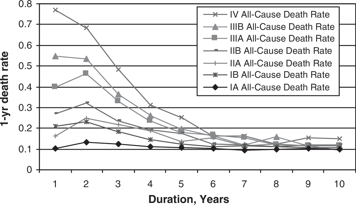
This figure shows the progression of all-cause mortality rates by duration. Higher stages have higher initial mortality, but the mortality rates converge after approximately 8 years.

Figure 2 shows, for selected cancer stages, the Figure 1 information by race. While blacks experience higher mortality rates in aggregate, stage is the primary determinant as early stage is associated with much lower mortality rates. We note that the higher mortality for small cell lung cancer is included in the Figure 2 mortality rates. Mortality rates for long-term survivors converge about 8 years after diagnosis.

FIG. 2.

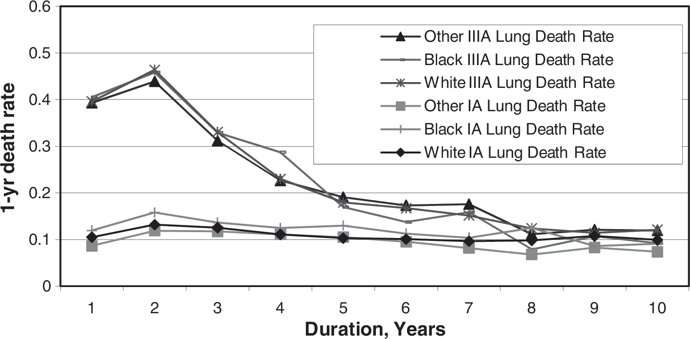
All-cause mortality rates for stages IA and IIIA by race. This figure shows detail behind selected cancer stages from Figure 1 by race. While blacks have higher aggregate all-cause mortality rates as well as mortality loads than whites, Figure 2 highlights that stage is the relatively dominant factor in mortality.

Though there are race-related mortality differences, stage at diagnosis is more important than race. Figure 2 does not address any racial disparities caused by diagnosis at a later stage. The supplemental material includes similar figures by age group, sex, and histologic type, which all point to the higher relative importance of stage compared to these other factors.

Figure 3 shows the reference mortality rates for the SEER cohorts by stage at diagnosis. The mortality rate shown each year reflects the reference mortality rates of the remaining survivors. We show the aggregate annual reference (population) mortality for each cohort, using each individual's age, sex, and race instead of the high mortality rates they actually experienced. Viewed this way, the differences in reference mortality among the stage cohorts are much smaller than the actual differences in Figure 1. This suggests that the cancer stage is the primary driver of the observed mortality rate differences—not differences in cohorts' age, sex, or race. The range of annual mortality rates (between 2% and 5%) is much lower than the mortality rate range shown in Figure 1. The higher reference mortality rates for stages IA and IB suggest older ages or a higher portion of males than the other stages. The initial decrease from year 1 to year 2 for stages IIIA, IIIB, and IV suggests that older patients or a higher portion of males died in the year of diagnosis. The relatively low reference mortality rate for the stage IV cohort suggests that these cancers, and especially their survivors, are younger or have more females than the other cohorts.

FIG. 3.

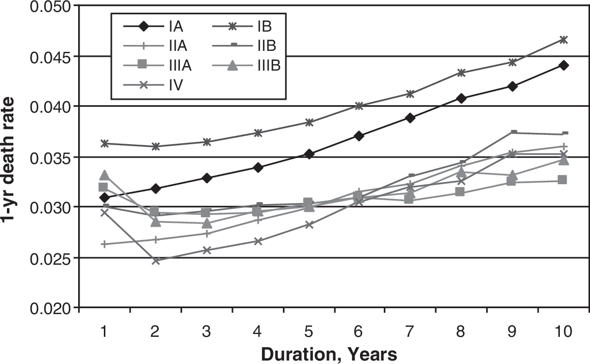
This figure shows the progression of reference population mortality rates by duration. The differences in the initial reference rates are due to different demographic mixes found in the stages. Each stage's reference mortality rate progresses with duration as the population ages.

Figure 4 shows the smoker and base reference mortality curves for the stage IA demographic, along with the observed mortality rates for stage IA and IIIA patients from Figure 1. The gap in mortality between stages of cancer at initial durations dwarfs the difference in mortality between reference mortalities and actual all-cause IA mortality. The smoker and reference mortality rates are certainly lower than the observed mortality of the cancer cohorts, but appear close to those of early stage lung cancers. Showing reference and smoker mortality in this way helps emphasize the proximity of the underlying population all-cause mortality. The all-cause smoker mortality curve is a useful comparison as about 87% of lung cancer deaths are attributable to smoking.²⁰

FIG. 4.

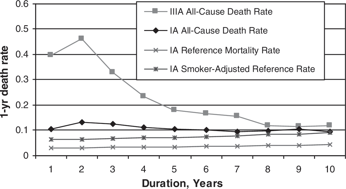
This figure juxtaposes higher all-cause mortality rates to various reference rates. It highlights that the stage is the biggest determinant of initial mortality. Stage IA's all-cause mortality rate is slightly higher than its reference rate and is even higher than the reference rate adjusted to a smoker population, but it is still significantly less than the IIIA all-cause mortality rate.

Figure 5 shows mortality ratios by stage and years since diagnosis. These are, in effect, the result of dividing the actual mortality rates in Figure 1 by the references rates in Figure 3. The mortality ratios decline as the duration increases, which presumably reflects cure rates and recovery from treatment. The 90% CIs shown around the mortality ratios reflect a normal approximation to the binomial distribution for mortality rates. The high ratios for the beginning durations of the later stages reflect the very high annual mortality rates for these cancers. The number of years required to obtain 90% of our data's total exposure-years, which is a measure of sample size by duration, is also shown; later stages have greater percentages of life-years in the first couple of years, indicating higher mortality in those stages.

FIG. 5.

Mortality loads with confidence intervals by stage and duration. This figure gives the reader a feel for where the bulk of our exposures lie. Later stages have greater percentages of life-years in the first couple of years, indicating higher mortality in those stages.

We applied the techniques described and the seriatim database of SEER survival and reference mortality to estimate the annual lives saved if Americans diagnosed with late stage lung cancers (IIIA, IIIB and IV) were, instead, diagnosed earlier with stage IA cancer and treated. This is not, of course, a complete or realistic analysis of screening, but it illustrates the power of the actuarial techniques to address important issues relevant to potential screening protocols.

With assumptions described in Tables 3 and 4, we found that in 2007, about 160,000 Americans were diagnosed with late stage lung cancer; by 2012 all but 8600 will be dead (Table 4). If these same people had their cancers detected as early stage lung cancers, a year or 2 before 2007, over 75,000 additional persons would be alive by 2012 (Table 4: Base Scenario). Assumptions that impute significantly slower progression between early stage and late stage lung cancers would still produce over 72,000 additional survivors by 2012 (Table 5). Assumptions of a 50% increase in mortality ratio for early stage lung cancer (which implies a worse outcome than SEER data implies for treated early stage lung cancers) and a slower progression between early stage and late stage would still produce over 36,000 additional survivors by 2012 (see Table 5 sensitivity).

Table 3.

Estimated 2007 Stage Distribution of Lung Cancer Patients in the United States

Stage	% in 2003 SEER	Reallocated	2007 US Population
I	19.3%	21.4%	45,567
II	2.8%	3.1%	6,698
III	29.2%	32.3%	68,994
IV	39.0%	43.2%	92,121
Unstaged	9.7%	N/A	N/A
Total	100.0%	100.0%	213,380

9.7% of patients in the original SEER database who were diagnosed in 2003 were unstaged. Allocating the unstaged patients across stages, we then used these proportions to assign the number of patients diagnosed with lung cancer by stage.

SEER, Surveillance, Epidemiology and End Results.

Table 4.

Model Results Showing Extra Survivors Attributable to Early Detection

Cohort	IIIA	IIIB	IV	Total LS
Model Inputs
Years between early stage and late stage diagnosis	1	1	2
Late stage years studied	5	5	5
Total years studied	6	6	7
Early stage	IA	IA	IA
Late stage	IIIA	IIIB	IV
Baseline Results
Total diagnosed with late stage in 2007	23,542	45,453	92,121	161,115
Total late stage survivors at end of study period	3,227	3,622	1,751	8,600
Total survivors at end of study period with early detection	12,251	22,948	49,341	84,540
Extra survivors attributable to early detection	9,024	19,326	47,590	75,940
% of survivors under current system	14%	8%	2%	5%
% of survivors with early detection	52%	50%	54%	52%
Sensitivity around Mortality Ratio (50% increase for early detection)
Total diagnosed with late stage in 2007	23,542	45,453	92,121	161,115
Total late stage survivors at end of study period	3,227	3,622	1,751	8,600
Total survivors at end of study period with early detection	8,066	14,812	31,948	54,826
Extra survivors attributable to early detection	4,840	11,190	30,197	46,226
% of survivors under current system	14%	8%	2%	5%
% of survivors with early detection	34%	33%	35%	34%

We found that over 75,000 lives of 2007-diagnosed lung cancer patients would be saved due to early detection of late stage (III and IV) cancer. This uses our baseline assumptions for lead time. Our sensitivity analysis shows a conservative estimate of over 46,000 lives saved with a 50% smaller difference in mortality ratios between the status quo and early detection. This is to account for possible pseudodisease and length bias. LS, late stage.

Table 5.

Alternative Model Results under Additional Lead Time Allowance

Cohort	IIIA	IIIB	IV	Total LS
Model Inputs
Years between early stage and late stage diagnosis	3	4	5
Late stage years studied	5	5	5
Total years studied	8	9	10
Early stage	IA	IA	IA
Late stage	IIIA	IIIB	IV
Results increasing lead time by 2-3 years from baseline scenario
Total diagnosed with late stage in 2007	23,542	45,453	92,121	161,115
Total late stage survivors at end of study period	3,227	3,622	1,751	8,600
Total survivors at end of study period with early detection	11,827	21,039	46,072	80,938
Extra survivors attributable to early detection	8,600	17,416	46,321	72,337
% of survivors under current system	14%	8%	2%	5%
% of survivors with early detection	50%	46%	52%	50%
Dual sensitivity: 50% increase on early detection mortality ratio and additional lead time allowance
Total diagnosed with late stage in 2007	23,542	45,453	92,121	161,115
Total late stage survivors at end of study period	3,227	3,622	1,751	8,600
Total survivors at end of study period with early detection	6,933	11,234	26,522	44,689
Extra survivors attributable to early detection	3,707	7,611	24,771	36,089
% of survivors under current system	14%	8%	2%	5%
% of survivors with early detection	29%	25%	29%	28%

This shows similar results but with expanded lead times. This is a more conservative scenario of lead time, but the extra survivors are still significant. LS, late stage.

We applied the actual and projected deaths developed by duration, or year, since diagnosis and modeled survivors for a study period of 5 years. Our baseline assumes a lead time of 1 year between stage IA and stages IIIA, IIIB, and 2 years between stages IA and IV. We projected the difference between those survivors in late stage and if they had been detected and treated at stage IA.

Other assumptions for lead time could easily be modeled in the same fashion, and we show the results for alternative lead time scenarios in Table 5. We also show an approach to sensitivity testing of other biases in the bottom half of Table 4.

We applied the incidence rates by stage from 2003 diagnoses in SEER, before our exclusions for those untreated or unstaged, to a 2007 national lung cancer incidences estimate of 213,380.²¹ These incidence rates result in 75.5% of cases with known stages to be stage III or IV. Table 3 shows the development of our stage distribution among the patients we tracked in SEER. Our assumed distribution differs somewhat from the published SEER summary statistics' distribution, but our staging follows the AJCC 3^rd edition guidelines, while SEER's Cancer Statistics Review uses a different staging method in its publication and reflects diagnoses between 1996 and 2003.²²

Model results

Table 4 shows the results of our modeling the late stage treated population in SEER if their lung cancers had been detected at stage IA. We have extrapolated our findings to the US population for 2007. We first describe baseline data on the modeled cohorts, then display our baseline estimates, and also show a stress scenario, under which the observed early stage mortality ratios were increased by 50%. This “stress” scenario addresses possible length bias or pseudodisease. Our Table 5 shows similar baseline and stress scenarios that address alternative assumptions for lead-time bias.

Figures 6 and 7A–C show late stage survivors by duration, along with survivors for the same cohorts if their lung cancers had been detected at an earlier stage. These correspond to the baseline scenario in Table 4 and assume an earlier detection at stage IA.

FIG. 6.

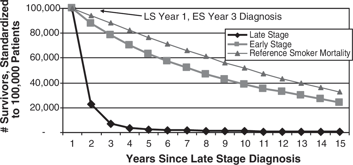
Modeled survivors curves for Stage IV cohort without lead time. This shows stage IV survivors by duration, along with survivors for the same cohort if their lung cancers had been detected at an earlier stage. Unlike the following Figures 7–9, Figure 6 does not assume any lead time between early stage and stage IIIA, which overstates the resulting mortality advantage of early detection. The mortality advantage by year can seen as the difference between the late stage (LS) curve and the hypothetical early stage (ES) detection curve at any given study year.

FIG. 7.

Modeled survivors for Stage IIIA, Stage IIIB, and Stage IV cohorts. (A) accounts for lead time and shows stage IIIA survivors by duration, along with survivors for the same cohort if their lung cancers had been detected at an earlier stage. These curves correspond to our model inputs for the baseline scenario, where early detection is defined as stage IA. (B) shows stage IIIB survivors by duration, along with survivors for the same cohort if their lung cancers had been detected at an earlier stage. (C) shows stage IV survivors by duration, along with survivors for the same cohort if their lung cancers had been detected at an earlier stage. ES, early stage; LS, late stage.

Earlier diagnosis is not free from mortality risk, and Figure 6 illustrates the need to account for the lead time required for earlier diagnosis of late stage cancers. Figure 6, which does not account for any lead time, compares survival of stage IV patients (late stage) to both their demographic counterparts' reference smoker survival rates and their counterparts' survival rates had they been diagnosed with stage IA cancer (early stage). Figure 6 does not account for lead time—it assumes the impossible event that early stage diagnosis could occur at the same time that late stage diagnosis currently occurs. This approach overstates the mortality advantage of early detection as no prior mortality is assumed.

Figures 7A–7C correct this distortion by applying lead time to stages IIIA, IIIB, and IV, respectively. We have applied lead time assumptions to show the impact of mortality despite earlier detection. We assume 1 year of lead time for stages IIIA and IIIB and 2 years for stage IV. In each figure, the distance between the late and early stage curves represents lives saved due to early detection assuming 100,000 cancer patients, and the distance between the early stage and reference smoker mortality curves represent lives lost relative to smoker mortality even with early detection. We back-modeled mortality of late stage cohorts to account for the theoretical deaths after early diagnosis.

Our modeled mortality for the 1 or 2 years of lead time in the late stage survival curve used the following assumptions:

75% weight to a smoker-adjusted reference population mortality, modified to reflect late stage demographics (ie, an older, more male population than the US average)

25% weight to earlier stage actual mortality

The first piece blends smoker and nonsmoker mortality rates to reflect the National Cancer Institute's estimate that 87% of lung cancer deaths are attributable to smoking.²³ The smoker load was based on implications from CDC-reported smoking-related deaths,^23,24 and was measured at 2.05 times reference mortality for an adult population. This developed smoker load was benchmarked against implications from National Center for Health Statistics data on smoking mortality.¹⁸

In scenarios with 2 years' lead time, the second piece of our modeled mortality uses stage IA SEER mortality for the first year (time = −1 on the x-axis) and IB mortality for the year immediately before late stage diagnosis (time = 0). For scenarios with higher lead time assumptions, we attributed the first half of the lead time to IA mortality and the second half to IB mortality. We also used an aging decrement, based on standard mortality average rates of change around late stage lung cancer average ages, to adjust the age of the cohort back to their age when the cancer was early staged. We used a similar method to roll back the ages of the early stage cohort. Finally, we shifted survivorship with early detection to reflect higher mortality ratios experienced at younger ages, since lead time will bring down the age at early stage diagnosis of the closed cohort.

Our baseline model assumes that late stage people would respond like SEER's stage IA people if their cancers were detected at stage IA. Some may argue that earlier detection of patients currently diagnosed with late stage cancer would yield higher mortality than the current IA cohort. Our stress scenario attempts to address this by increasing the IA mortality rate by 50%. We show the model results for other lead time assumptions in Table 5.

Discussion

Lung cancer is a disease for which improved outcomes have been modest. There is considerable interest in early detection approaches but there are formidable analytical challenges to reliably determining outcomes. We have used actuarial techniques to examine issues of potential benefit for lung cancer screening as an example of the potential utility of this analytical approach.

Use of mortality ratios to test biases associated with screening

Table 6 shows how mortality ratios can be used to test assumptions about pseudodisease, length bias, and very aggressive cancers. The percentages show the portion of patients in our early stage cohort with various combinations of “biases” needed to produce the higher mortality reflected in our stress scenario. For pseudodisease, we assumed a mortality ratio of 1.0 (standard population). For length-biased people, we assumed the observed mortality ratio of stage IA at duration 10. To model people with aggressive cancer, we assigned a mortality ratio of stage IIIA people. There are, of course, an infinite number of possible combinations of the 3 factors that produce the 50% higher mortality.

Table 6.

Sample Sets of Distribution of Biases that Lead to a Mortality Ratio Increase of 50%

	Distribution of Patients
Scenario	A	B	C
Pseudodisease	0%	20%	61%
Length Bias (early stage at duration t = 10)	68%	46%	0%
Advanced Stage (Neither Bias)	32%	34%	39%
Total	100%	100%	100%

These are 3 scenarios of the prevalence of biases apart from lead time that result in a mortality ratio increase of 50%, which is our assumption in the sensitivity analysis found in Tables 4 and 5. We believe it unlikely for such a high portion of patients in the SEER database to be attributable to pseudodisease or slow-growing cancers (length bias).

SEER, Surveillance, Epidemiology and End Results.

Pseudodisease is probably not an issue with SEER, as the cases are confirmed. Scenario A in Table 6 shows that, assuming no pseudodisease, it would take a combination of 68% slow growing and 32% advanced stage (IIIA) mortality to produce our stress scenario.

Our source data with all-cause mortality in this article seems to enter the controversy over use of all-cause mortality as a clinical trial end point for screening, which has been termed “hopelessly inefficient.”²⁵ Indeed this article's use of all-cause mortality applies to both principal data sources: SEER data and normative population mortality. However, we use these data to make inferences about stage and mortality, with possible public health applications rather than inferences about clinical trial data. Perhaps some of the findings in Table 1 and Table 2 would be difficult to obtain in the context of a randomized controlled trial—for example, that the extra mortality burden associated with lung cancer diagnosis is higher for blacks than whites for both sexes, for both non-small cell and small cell cancers, and that the discrepancy appears to be driven by racial differences in stage distribution. In this regard, actuarial approaches would complement the information derived from randomized screening trial sources.

The mortality ratios found in Table 2 stand as a proxy for the derived extra burden associated with lung cancer, its treatment, and its side effects. These ratios are the all-cause mortality rates found in Figure 1 divided by the reference population mortality rates in Figure 3. The strikingly consistent progression of these mortality ratios by stage demonstrates the success of staging as a meaningful measure for all-cause mortality. Higher stage is profoundly associated with higher all-cause mortality—stage has real meaning for society beyond arbitrary definitions based on tumor size. Similarly, earlier stage is profoundly associated with lower mortality. Applying this knowledge to screening will require additional research to explore the potential of sojourn time improvement through screening⁹ and resolution of critical issues related to overdiagnosis likely associated with earlier stages.²⁶

While the limitations of population data to determine causality among risk factors are recognized, the large, credible population sizes and years of follow-up available through SEER data and mortality tables dwarf those available through randomized controlled trials. Of course, for population data to yield useful comparative information, they should be appropriately normalized, as our methodology does when we compare stages and other factors.

An important caveat, however, is that the reader should consider whether therapeutic changes since the time period of the population data or local practice patterns different from the SEER sites affect the applicability of this work.

The insurance industry relies on actuarial techniques to recognize and manage the risk associated with individuals' differing mortality risks and to maintain life insurance company solvency in highly competitive markets. Actuarial techniques originated over a century ago and often involve establishing mortality ratios—relationships between a subpopulation's mortality rates and reference mortality rates. Not surprisingly, underwriters of life insurance policies focus on mortality rather than survival, and mostly on all-cause mortality. This perhaps corresponds well to patients' interests, as cancer patients may not appreciate distinctions between death from cancer, from treatment side effects, or from something else.

We note that our approach may gain relevance given the recent interest in measuring the “cure of cancer” using cure models as an improvement over traditional survival analysis of registry data.²⁷ These models define cured patient populations as those having the same mortality as the rest of the population after adjustment for age and sex. In this sense, the convergence of the mortality ratio of survivors close to 1.0 shown in Figures 1 and 2 represent cured patients. We note that the curves in Figures 6 and 7A–7C do not converge. However, these figures show the number of survivors by year, not the annual mortality rates. The higher number of survivors for early stage lung cancer reflects the dismal survival of patients with late stage lung cancer. The lower number of survivors for early stage lung cancer than for smokers reflects the higher initial mortality rates for early stage lung cancer than for smokers. However, the smoker and early stage curves appear to become close to parallel (have similar declining slopes), which indicates that the mortality rates of these 2 populations converge.

The stage differences in mortality ratios apparent in Table 2 suggest the value of mortality as a measurable outcome in cancer-related population health management programs. The mortality ratio approach may constitute an informative measure of important parameters such as disparities and progress in treatment, diagnosis, and prevention. This approach has recently been applied to differences in cancer outcomes of European countries.²⁸ Table 2 identifies important differences between men and women and between patients who are classified as white, black, or other races; similar analysis has demonstrated treatment and survival differences for Hispanics and whites for early stage lung cancer.²⁹ Large population health management programs that incorporate cancer screening can use mortality ratios as an outcomes measure, and geographic differences in mortality ratios should reflect geographic differences in screening, treatment, and prevention. In addition, we propose actuarial modeling as a pragmatic tool to evaluate new management approaches such as with lung cancer screening programs and other new clinical management approaches.

Population health management programs have had to address a number of methodological issues including regression to the mean, differential disease/nondisease trends, and selection bias. Most current programs focus on noncancer chronic conditions such as congestive heart failure, chronic obstructive pulmonary disease, diabetes, coronary artery disease, and asthma. As these programs expand to address cancer and cancer screening, they will face additional controversies, including lead-time bias, pseudodisease, and pseudodiagnosis. As described above, the actuarial application, by virtue of its validation with vast numbers of cases as shown in Figures 6 and 7A–7C, can help address these complex issues.

Many actuarial techniques reference underlying benchmark data developed from very large data sets.³⁰ We use that approach here by comparing lung cancer mortality rates to expected general population mortality rates, which are considered normative.¹³ This allows comparing the actual mortality rates of individuals in the SEER lung cancer records¹² to reference mortality rates adjusted for individuals' age, sex, and race. Using reference data in this way avoids the difficulty of matching individuals to controls with the same age, sex, and race. It also avoids the noise of statistical fluctuations, at least from the normative data used in place of controls. The actuarial techniques we use in this paper produce comparisons of subpopulations from the large SEER data set, and these techniques can avoid some of the weaknesses reported for observational studies.³¹ The authors hope our application of these techniques will shed new light on how the mortality of patients with lung cancer varies with stage at diagnosis, histology, age, sex, and other factors, and how that mortality varies from standard mortality rates adjusted for age, sex, race, and year of death.³²

Similar approaches can be used when mortality is an important outcome. Mortality rates are very high in this example and in a similar study of hospice.³³ However, comparisons to standard population mortality tables can also be useful when expected death rates are low and volatility in the control arm may overwhelm comparisons. Using a population mortality table based on the experience of millions of lives offers the potential to remove variability from the control side to an extent that would require an impractically large control group. This approach may be of value when evaluating a technology across time intervals, such as different generations of spiral CT scanners or other analytical instrumentation that are heavily dependent on computational speed.³⁴ These technologies can experience rapid technical evolution that outstrips the time required to conduct a formal randomized comparison. Further, actuarial approaches may also provide a useful approach for those situations in which it is unethical to construct a control group.

The potential impact of population health management on mortality would seem to be a fruitful area for the mortality ratio approach. In particular, it is sometimes unclear how to compare efforts aimed at preventing versus better managing cases. The federal Medicare program could gain important insight on prioritizing prevention/intervention efforts among other major chronic diseases (eg, chronic obstructive pulmonary disease, congestive heart failure, diabetes) by examining mortality ratios by age for newly diagnosed cases and existing cases.

Familiarity with actuarial techniques and terminology may help medical researchers better influence health care decision makers. The vast majority of medical spending flows through private or social insurance programs, and the financial and administrative leadership of these programs more often speak in actuarial terms than academic ones.

Conclusion

Life insurance actuarial techniques, applied to SEER data, offer a useful tool to create descriptive statistics about all-cause survival relative to normal population mortality patterns. These techniques also provide a convenient approach to modeling the impact of issues critically important to the evaluation of detection approaches that may identify cancers at earlier stages. These techniques also provide reference mortality rates that may help physicians, patients, and payers better understand cancer patients' mortality risks.

This article illustrates how life insurance actuarial techniques can be used to compare early stage and late stage lung cancer mortality. Other actuarial techniques, typically used in health insurance and managed care, can be applied to investigate the cost issues surrounding early lung cancer management.

Footnotes

Disclosure Statement

Ms Goldberg, Mr Mulshine, Mr Hagstrom, and Mr Pyenson disclosed no conflicts of financial interest. Ms. Goldberg, Mr. Hagstrom, and Mr. Pyenson were supported in this work by grants from Lung Cancer Alliance, American Legacy Foundation, Bonnie J. Addario Lung Cancer Foundation, Joan's Legacy Foundation, LUNGevity Foundation, Prevent Cancer Foundation, and Thomas G. Labrecque Foundation.

References

Jemal

, Siegel

, Ward

et al. Cancer statistics, 2008. CA Cancer J Clin, 2008; 58:71–96.

Henschke

, Yankelevitz

, Libby

, Pasmantier

, Smith

, Miettinen

. Survival of patients with stage I lung cancer detected on CT screening. N Engl J Med, 2006; 355:1763–1771.

Goldstraw

, Crowley

, Chansky

et al. The IASLC Lung Cancer Staging Project: Proposals for the revision of the TNM stage groupings in the forthcoming (seventh) edition of the TNM Classification of Malignant Tumours. J Thorac Oncol, 2007; 2:706–714.

Rami–Porta

, Ball

, Crowley

et al. The IASLC Lung Cancer Staging Project: Proposals for the revision of the T descriptors in the forthcoming (seventh) edition of the TNM classification for lung cancer. J Thorac Oncol, 2007; 2:593–602.

Bach

, Silvestri

, Hanger

et al.

Screening for lung cancer: ACCP Evidence-Based Clinical Practice Guidelines (2nd Edition)

Chest, 2007; 132:69–77.

Henschke

, Yankelevitz

. CT screening for lung cancer: Update 2007. Oncologist, 2008; 13:65–78.

Bach

, Jett

, Pastorino

, Tockman

, Swensen

, Begg

. Computed tomography screening and lung cancer outcomes. JAMA, 2007; 297:953–961.

McMahon

, Kong

, Johnson

et al. Estimating long-term effectiveness of lung cancer screening in the Mayo CT screening study. Radiology, 2008; 248:278–287.

Chien

, Chen

. Mean sojourn time and effectiveness of mortality reduction for lung cancer screening with computer tomography. Int J Cancer, 2008; 122:2594–2599.

10.

Habbema

JDF

, Schechter

, Cronin

, Clarke

, Feuer

. Modeling cancer natural history, epidemiology, and control: Reflections on the CISNET breast group experience. J Natl Cancer Inst Monogr, 2006; 36:122–126.

11.

Lee

. Screening mammography: Proven benefit, continued controversy. Radiol Clin North Am, 2002; 40:395–407.

12.

Surveillance, Epidemiology, End Results (SEER) Program. www.seer.cancer.gov SEER*Stat Database: Incidence—SEER 9 Regs Limited-Use, Nov 2006 Sub (1973–2004), National Cancer Institute, DCCPS, Surveillance Research Program, Cancer Statistics Branch, released April 2007, based on the November 2006 submission. http://seer.cancer.gov/data/access.html. 2007 Oct 17.

13.

Batton

. Mortality Table Construction. Englewood Cliffs, NJ: Prentice-Hall, Inc., 1978; 221.

14.

Collaborative Staging Task Force of the American Joint Committee on Cancer. Collaborative Staging Manual and Coding Instructions, Part I, Version 01.03.00. NIH Publication Number 04-5496. Bethesda, MD: National Institutes of Health, 2006.

15.

Lababede

, Meziane

, Rice

. TNM staging of lung cancer: A quick reference chart. http://chestjournal.org/cgi/content/abstract/115/1/233. 2008 April 21.

16.

CDC seriatim mortality tables. http://www.census.gov/popest/archives/index.html. 2008 February 23.

17.

CDC race-specific tables. Prior to 1999, Table HIST290, Death Rates for Selected Causes by 10-Year Age Groups, Race, and Sex: Death Registration States, 1900–1932, and United States, 1933–1998. http://www.cdc.gov/nchs/datawh/statab/unpubd/mortabs/hist290.htm. 2008 April 20 Between 1999-2004, Table GMWK310, Deaths by Single Years of Age, Race, and Sex: United States, 1999–2004. http://www.cdc.gov/nchs/datawh/statab/unpubd/mortabs.htm. 2008 April 20.

18.

Centers for Disease Control and Prevention. Current cigarette smoking among adults 18 years of age and over, by sex, race, and age: United States, selected years 1965–2005. Table 63. http://www.cdc.gov/nchs/products/pubs/pubd/hus/healthrisk.htm. 2008 April 20.

19.

Ries

LAG

, Melbert

, Krapcho

et al. SEER Cancer Statistics Review, 1975-2005, Section 0-17. National Cancer Institute. http://seer.cancer.gov/csr/1975_2005/Based on November 2007 SEER data submission, posted to the SEER Web site, 2008.

20.

Cowell

, Hirst

. Mortality differences between smokers and nonsmokers. Trans Society Actuaries, 1980; 32:193.

21.

Report of the Task Force on Smoker/Nonsmoker Mortality. Trans Society Actuaries, 1982; 34:345.

22.

Bowers

, Gerber

, Hickman

, Jones

, Nesbit

. Actuarial Mathematics. Schaumburg, IL: Society of Actuaries, 1997; 79 82.

23.

National Cancer Institute. Cigarette smoking and cancer: Questions and answers. http://www.cancer.gov/cancertopics/factsheet/tobacco/cancer. 2008 November 4.

24.

American Cancer Society, Inc. Surveillance Research. Cancer facts and figures 2007. http://www.cancer.org/downloads/STT/CAFF2007PWSecured.pdf. 2008 April 21.

25.

National Cancer Institute. SEER Cancer Statistics Review 1975-2004, Section 15 Lung and Bronchus, Table XV-9. http://seer.cancer.gov/csr/1975_2004/results_merged/sect_15_lung_bronchus.pdf. 2010 January 23.

26.

Annual Smoking-Attributable Mortality, Years of Potential Life Lost, and Productivity Losses—United States, 1997–2001. http://www.cdc.gov/mmwr/preview/mmwrhtml/mm54245a1.htm. 2008 March 26.

27.

Cigarette Smoking Among Adults—United States 2006. http://www.cdc.gov/mmwr/preview/mmwrhtml/mm5644a2.htm. 2008 March 26.

28.

Tabar

, Duffy

, Yen

M–F

et al. All-cause mortality among breast cancer patients in a screening trial: Support for breast cancer mortality as an end point. J Med Screen, 2002; 9:159–162.

29.

Black

. Overdiagnosis: An underrecognized cause of confusion and harm in cancer screening. JNCI, 2000; 92:1280–1282.

30.

Francisci

, Capocaccia

, Grande

et al. The cure of cancer: A European perspective. Eur J Can, 2009; 45:1067–1079.

31.

Berrino

, Verdecchia

, Lutz

et al. Comparative cancer survival information in Europe. Eur J Can, 2009; 45:901–908.

32.

Wisnivesky

, McGinn

, Henschke

et al. Ethnic disparities in stage 1 non-small cell lung cancer. Am J Respir Crit Care Med, 2005; 171:1158–1163.

33.

Klugman

, Panjer

, Willmot

. Loss Models, From Data to Decisions, 2nd. New York: John Wiley and Sons, 2004preface.

34.

Giordano

, Kuos

, Duan

et al. The limits of observational data in determining outcomes from cancer therapy. Cancer, 2008; 112:2456–2466.

35.

Centers for Disease Control and Prevention. Seriatim mortality tables. http://www.census.gov/popest/archives/index.html. 2008 February 23.

36.

Connor

, Pyenson

, Fitch

. Comparing hospice and nonhospice patient survival among patients who die within a three-year window. J Pain Symptom Manage, 2007; 33:238–246.

37.

Mulshine

, Sullivan

. Clinical practice. Lung cancer screening. NEJM, 2005; 352:2714–2720.