Are Meals at Full-Service and Fast-Food Restaurants “Normal” or “Inferior”?

Abstract

Whereas some studies show statistically significant linear associations between consumption at full-service restaurants and consumer incomes, studies of fast-food restaurants fail to find statistically significant linear associations. In this study, nationally representative data were drawn from the 1994–1996 Continuing Survey of Food Intakes by Individuals and the accompanying Diet and Health Knowledge Survey. The sample contained 4972 individuals who were 21 years of age or older. Dependent variables measured number of restaurant visits on 2 nonconsecutive days. Income was total annual household income. Control variables reflected sociodemographic, economic, lifestyle, and attitudinal variables. To capture possible curvilinear relationships between income and food consumption, we analyzed frequency distributions, regressions on full samples including income squared, and we divided samples into above- and below-average income groups. Zero-inflated negative binomial regressions accounted for excessive zeros within dependent variables. We found that fast-food restaurants were “normal goods” for below-average income, but “inferior goods” for above-average income, whereas full-service restaurants were “normal” for virtually all income levels. Earlier studies were flawed because they only tested for linear associations. Our results have implications for the poverty and obesity debate. (Population Health Management 2011;14:307–315)

Introduction

O ver the past 25 years, Americans have been consuming an increasingly significant portion of their total calories at restaurants.¹ Research has shown that restaurant food has a higher percentage of fat compared to food prepared at home.² Consequently, the proliferation of fast-food restaurants across the American landscape in recent decades is frequently cited as one cause of rising obesity rates.^3
–5 Yet full-service restaurants are not cited as frequently.

Studies suggest that obesity and income are negatively correlated.^6,7 Persons on limited budgets are more likely to frequent fast-food restaurants than full-service ones. The low cost of fast food is alleged to partially explain the negative correlation.⁸ Yet studies report weak, inconsistent, and contradictory monotonic associations between family income on the one hand and either total spending on fast food or frequency of visits to fast-food restaurants on the other.^9,10 Although some evidence suggests that family income and visits to full-service restaurants are positively correlated in linear models, the statistical methods used to arrive at this conclusion could be improved.⁹

The goal of this research is to clarify these relations by testing whether the association between family income and restaurant visits is monotonically increasing or shaped like an inverted “U.” In economics, if consumption of a good rises as income rises, that good is said to be “normal”; if consumption falls, it is said to be “inferior.” In economics textbooks, normal and inferior are frequently explained with food examples. For example, Perloff¹¹ uses hamburger and steak. He suggests that for families in lower income ranges, rising income may be associated with much greater consumption of hamburger and a small increase in the consumption of steak. For families in the upper income ranges, rising incomes may be associated with falling consumption of hamburger and continued rising consumption of steak. In this case, hamburger is normal up to some middle level of income but inferior for income above that threshold; steak is normal throughout all levels of income.

We tested the Perloff conjecture as it applies to fast-food and full-service restaurants. Our hypothesis was that fast-food visits initially increase with family income but ultimately reach a peak and then begin to fall (ie, fast-food visits and income display an inverted “U” shape when income is measured along the horizontal axis). We also hypothesize that full-service visits and income display a monotonically increasing relation; an upward sloping line or curve.

To test our hypothesis, we used an innovative regression technique: the zero-inflated negative binomial model. Our dependent variables were “count” data (ie, data that take on values such as 0 visits, 1 visit, 2 visits). In addition, a disproportionate number of our data points (observations) were zeros. For data like these, linear regression generates inconsistent estimates. The zero-inflated negative binomial is designed precisely for data with these characteristics and provides consistent estimates.

Methods

Data

Data were drawn from the 1994-1996 Continuing Survey of Food Intakes by Individuals (CSFII) and the accompanying Diet and Health Knowledge Survey (DHKS).¹² The CSFII collected information on foods eaten, nutritional content, and where foods were obtained, for a nationally representative sample of US noninstitutionalized persons (n = 16,103). The dietary data consisted of 2 nonconsecutive days (3 to 10 days apart) that were collected between January 1994 and January 1997 during in-person interviews in the respondent's home, using 24-hour recall. The DHKS was a follow-up telephone survey with a subsample of 5765 adults, 21 years of age or older. The DHKS contained information about respondents' knowledge and attitudes toward dietary guidance and health.¹³ Our sample was restricted to 4972 subjects, 21 years of age or older, who had complete information in the DHKS on the variables we required. Dependent variables measured number of visits (most frequently 0, 1, or 2) to either full-service or fast-food restaurants. Following Binkley,¹⁰ we used visits to represent complete meals.

Based on previous literature, 4 groups of independent variables were used: sociodemographic variables, economic variables, health habits, and attitudinal variables. Most previous literature includes only sociodemographic and economic variables.

Sociodemographic variables included age, age squared, sex, race, education level, status of the household head, family size, region, and urban environment.

Economic variables included household income, food stamps, and working hours per week. Income was measured as the total annual dollar amount of household income. An indicator (yes/no) measured food stamps. The food stamp variable was included to account for 2 possible effects. First, people with food stamps may feel richer than their counterparts and, therefore, increase restaurant visits. On the other hand, people with food stamps essentially face lower food prices from supermarkets than people without food stamps and these lower supermarket prices might translate into greater food intake from supermarkets and lower intake from restaurants.

The third group of independent variables was related to risk factors for many diseases, individual willpower, self-control, and individual heterogeneity, generally. These variables included regular exercise, smoking, drinking, hours spent watching TV, and obesity status. Although these variables are rare in prior literature on visits or spending at restaurants, we felt they were significant because they are frequently included in other analyses to explain individuals' health and propensity for disease.⁶ Obesity might be viewed as endogenous. We nevertheless included an obesity variable, reasoning that it should help reduce unobservable heterogeneity associated with time preference.¹⁴ But our conclusions remained unchanged for results that did not include obesity.

Binkley¹⁰ included variables for individual knowledge, concerns, and attitudes toward nutrition as well as weekend day (Friday, Saturday, Sunday). The effect of individual knowledge, concerns, and attitudes about food away from home is not our main concern. Thus, from among Binkley's variables,⁹ we included only variables for weekend day and indicator variables if either the price or convenience of buying food was “important” to the respondents. In additional results that included all of Binkley's variables on knowledge, concerns, and attitudes toward nutrition, our conclusions were not altered.

The rationale for including control variables is provided in other studies^9,10; therefore, we limit our comments on control variables. Work hours is an indirect measure of the individual's value of time⁶ and we, therefore, expected work hours to be positively correlated with visits to both fast-food and full-service restaurants.¹⁰ We were concerned with unobservable heterogeneity. Psychosocial orientations such as time and risk preferences may systematically vary across income groups. We attempted to measure these orientations directly with 2 questions in the DHKS that reflect respondents' attitudes toward the “importance” of price or the convenience of eating out. We also attempted to measure them indirectly by adding variables on exercise, smoking, and dietary intake.

Method

Linear regression was not used because dependent variables were “count data,” not normally distributed, and because linear regression could lead to negative predicted values. Log-linear regressions were deemed to be inappropriate because the log of zero is undefined. Figure 1 shows the distribution of visits. Poisson models are frequently suggested for count data.¹⁴

FIG. 1.

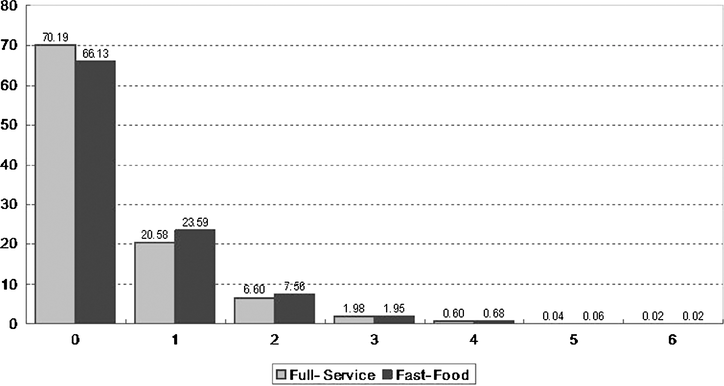
Number of table-service and fast-food restaurant visits. Values on Y-axis indicate % and X-axis indicate frequency.

Under the Poisson assumption, the probability of having y visits by individual i is given by \documentclass{aastex}\usepackage{amsbsy}\usepackage{amsfonts}\usepackage{amssymb}\usepackage{bm}\usepackage{mathrsfs}\usepackage{pifont}\usepackage{stmaryrd}\usepackage{textcomp}\usepackage{portland, xspace}\usepackage{amsmath, amsxtra}\pagestyle{empty}\DeclareMathSizes{10}{9}{7}{6}\begin{document}\begin{align*}{\rm Pr} [y_i|X_i] = \frac {e^ {- \lambda_i} \lambda_i^ {y_i}}{y_i!}, \quad y_i = 0, 1, 2, \ldots \ {\rm and} \ i = 1, 2, 3, \ldots, {\rm n} \tag {{\rm Eq.} \ 1} \end{align*}\end{document}

and a population mean is given by \documentclass{aastex}\usepackage{amsbsy}\usepackage{amsfonts}\usepackage{amssymb}\usepackage{bm}\usepackage{mathrsfs}\usepackage{pifont}\usepackage{stmaryrd}\usepackage{textcomp}\usepackage{portland, xspace}\usepackage{amsmath, amsxtra}\pagestyle{empty}\DeclareMathSizes{10}{9}{7}{6}\begin{document}\begin{align*} \lambda_i = \exp (X_i^{\prime} \beta), \tag{{\rm Eq.}\ 2} \end{align*}\end{document}

where X is a set of explanatory variables with corresponding coefficients, β, and “!” denotes factorial.

But the Poisson model has drawbacks. It assumes the variance equals the mean. In numerous applications, however, the variance of Poisson models underestimates the actual variance.¹⁵ When the variance is greater than the mean, the distribution is said to display “overdispersion.” The standard parametric model to account for overdispersion is the negative binomial model. The negative binomial may be interpreted as a Poisson distribution with unobserved heterogeneity that, in turn, can be conceptualized as a mixture of 2 probability distributions, Poisson and gamma.¹⁵ Unlike the Poisson, the negative binomial does not assume that all individuals have an equal chance of, in our case, visiting a restaurant. Certain groups of individuals in the population are more prone than others to visit a restaurant. Variability in the population not measured by typical covariates (unobserved heterogeneity) causes the variance to be larger than the mean (ie, population heterogeneity causes overdispersion). The negative binomial distribution that accounts for overdispersion in the Poisson adds a parameter, α, that reflects unobserved heterogeneity, \documentclass{aastex}\usepackage{amsbsy}\usepackage{amsfonts}\usepackage{amssymb}\usepackage{bm}\usepackage{mathrsfs}\usepackage{pifont}\usepackage{stmaryrd}\usepackage{textcomp}\usepackage{portland, xspace}\usepackage{amsmath, amsxtra}\pagestyle{empty}\DeclareMathSizes{10}{9}{7}{6}\begin{document}\begin{align*}{\rm Pr} (y_i|X_i) = \frac {\Gamma (y_i + \alpha^ {- 1})} {y_i! \Gamma (\alpha^ {- 1})} \left(\frac {\alpha^ {- 1}} {\alpha^ {- 1}+ \lambda_i} \right) ^ {\alpha^ {- 1}} \left(\frac {\lambda_i}{\alpha^ {- 1} + \lambda_i} \right) ^ {y_i} \tag {{\rm Eq.} \ 3} \end{align*}\end{document}

where Γ(•) is the gamma function and the dispersion parameter must be greater than or equal to zero, α ≥ 0. Equation 4 reduces to the Poisson if α = 0. If the dispersion parameter is significantly greater than zero, the data are overdispersed and are better estimated with a negative binomial model. Our data indicated overdispersion. (Full service: Prob > = chibar2 = 0.00 for LR test of alpha = 0; Fast food: Prob > = chibar2 = 0.00 for LR test of alpha = 0).

Another concern for our dependent variables was the possibility that the number of zeros may be excessive. Respondents were asked where each meal was eaten during 2 nonconsecutive days. A “zero” response could have arisen from 2 separate groups of people. The first group might never visit restaurants. The second group might visit them, but may not have done so on the 2 days specified by the data gatherers. A “zero” for the second group underestimates their tendency for visits, and therefore would result in an inflated number of zeros in the data. Neither the Poisson nor the simple negative binomial account for the 2 different groups. A zero-inflated negative binomial model, however, accounts for excessive zeros.¹⁵

The zero-inflated negative binomial model combines 2 different data-generating processes (called “dual regime”). First, a binary model (logistic) determines whether visits are zero or greater than zero. Second, the simple negative binomial governs the actual number of visits. The zero-inflated negative binomial model combines both and the density function for observation i is \documentclass{aastex}\usepackage{amsbsy}\usepackage{amsfonts}\usepackage{amssymb}\usepackage{bm}\usepackage{mathrsfs}\usepackage{pifont}\usepackage{stmaryrd}\usepackage{textcomp}\usepackage{portland, xspace}\usepackage{amsmath, amsxtra}\pagestyle{empty}\DeclareMathSizes{10}{9}{7}{6}\begin{document}\begin{align*}{\rm Pr} (y_i|X_i) = p_i + (1 - p_i) \left(\frac {\alpha^ {- 1}}{\alpha^ {- 1} + \lambda_i} \right) ^ {\alpha^ {- 1}} \quad {\rm if} \ y_i = 0 \tag {{\rm Eq.} \ 4} \end{align*}\end{document} \documentclass{aastex}\usepackage{amsbsy}\usepackage{amsfonts}\usepackage{amssymb}\usepackage{bm}\usepackage{mathrsfs}\usepackage{pifont}\usepackage{stmaryrd}\usepackage{textcomp}\usepackage{portland, xspace}\usepackage{amsmath, amsxtra}\pagestyle{empty}\DeclareMathSizes{10}{9}{7}{6}\begin{document}\begin{align*}{\rm Pr} (y_i|X_i) = &(1 - p_{i}) \frac {\Gamma (y_{i} + \alpha^{- 1})} {y_{i}! \Gamma (\alpha^{- 1})} \left(\frac {\alpha^{- 1}}{\alpha^{-1} + \lambda_{i}} \right) ^{\alpha^{-1}} \left(\frac{\lambda_i} {\alpha^{-1} + \lambda_{i}} \right) ^{y_{i}} \\&{\rm if} \ y_{i} > 0 \tag{{\rm Eq.} \ 5} \end{align*}\end{document}

where p_i is the probability of a zero count in the binary logistic model.

The zero-inflated negative binomial distribution approaches the negative binomial if p = 0, and approaches the Poisson if both a = 0 and p = 0. We ran Vuong tests¹⁶ and determined that our data did have excessive zeros. Our Vuong tests used age, age squared, and sex as covariates (Vuong test of zero-inflated negative binomial vs. standard negative binomial for full service: z = 2.02 [P < 0.05]; Vuong test of zero-inflated negative binomial vs. standard negative binomial for fast-food: z = 2.33[P < 0.05]). The zero-inflated negative binomial model accounted for unobserved heterogeneity, overdispersion, and excessive zeros.

Our critical independent variable was income. We tested for nonlinear income associations with 3 methods. In the first we simply visually inspected histograms for full-service and fast-food restaurant visits for 10 income categories. The second method included income and income squared as covariates for the all-incomes sample, including those with below- and above-average incomes. The third method divided the sample in 2 (persons with below-average income and persons with above-average income) and ran separate regressions on each subsample. In the third method, log of income was the independent variable; the first and second methods did not take the log. We used log of income to allow easy calculation of elasticities. Using log of income in the second method with income squared would have unnecessarily complicated estimation of the possible inverted “U” curve.¹⁷

We calculated incidence rate ratios for binary covariates and elasticities for continuous and binary covariates using coefficients and sample means. The incidence rate ratio for a 1-unit change in X_j with all other covariates held constant is \documentclass{aastex}\usepackage{amsbsy}\usepackage{amsfonts}\usepackage{amssymb}\usepackage{bm}\usepackage{mathrsfs}\usepackage{pifont}\usepackage{stmaryrd}\usepackage{textcomp}\usepackage{portland, xspace}\usepackage{amsmath, amsxtra}\pagestyle{empty}\DeclareMathSizes{10}{9}{7}{6}\begin{document}$$e^{\beta_i}$$\end{document} . Incidence rates are easily interpreted. For example, an incidence rate of 1.193 on a “male” variable means that males had a rate 1.193 times greater than females for the number of full-service restaurant visits.

Coefficients in the zero-inflated negative binomial, after being multiplied by 100, can be interpreted as the change in the log of expected counts divided by a 1-unit change in the covariate. If the covariate, too, is expressed as a log, then the estimated coefficient is an elasticity (ie, percentage change in number of visits divided by percentage change in covariate).

All analyses were conducted using Stata software (Stata Corp LP, College Station, TX).

Results

Descriptive statistics

Table 1 provides means for the all-incomes sample as well as for subsamples with below- and above-average income. The sample mean income in the full sample was $35,628. Compared to respondents in the below-average subsample, respondents in the above-average subsample had incomes about 3.5 times larger, worked more hours, had higher levels of education, and larger household size. Fewer than 1% in the above-average subsample reported receiving food stamps. Higher proportions of the above-average group exercised, drank, and were white and male, whereas a higher percentage of the below-average group smoked, watched TV, were obese, and were relatively more concerned with food prices and convenience. Overall, these means and percentages are what would be expected in a representative sample of US families, thus lending credence to our data.

Table 1.

Descriptive Statistics of Variables: Definitions, Means, and Standard Deviations of Variables

		All-incomes Sample		Below-average income sample		Above-average income sample
Definition		N = 4972		N = 2962		N = 2010
TSFOOD	Number of full-service restaurant visits	0.424	(0.762)	0.324	(0.680)	0.572	(0.848)
FASTFOOD	Number of fast-food restaurant visits	0.477	(0.786)	0.417	(0.756)	0.566	(0.820)
Income	Household income	35628	(26521)	17554	(9296)	62262	(20535)
Age	Age in years	50.535	(17.03)	52.578	(18.53)	47.525	(14.03)
Age Squared	Age squared	2844.0	(1787)	3107.7	(1962)	2455.4	(1405)
Male	= 1 if male	0.502	(0.500)	0.467	(0.499)	0.555	(0.497)
White	= 1 if White	0.826	(0.379)	0.779	(0.415)	0.896	(0.306)
Asian	= 1 if Asian	0.015	(0.123)	0.011	(0.103)	0.022	(0.148)
Other races	= 1 if other races	0.044	(0.206)	0.060	(0.238)	0.021	(0.145)
Education	Years of education completed	12.744	(3.010)	11.804	(3.051)	14.129	(2.340)
Head	= 1 if household head	0.947	(0.225)	0.956	(0.206)	0.933	(0.250)
Household Size	Household size	2.592	(1.453)	2.375	(1.442)	2.911	(1.411)
East	= 1 if lives in East region	0.190	(0.392)	0.174	(0.379)	0.214	(0.410)
Midwest	= 1 if lives in Midwest region	0.252	(0.434)	0.254	(0.435)	0.249	(0.432)
South	= 1 if lives in South region	0.356	(0.479)	0.380	(0.485)	0.321	(0.467)
Rural	= 1 if lives in rural area	0.267	(0.442)	0.313	(0.464)	0.200	(0.400)
Urban	= 1 if lives in urban area	0.294	(0.456)	0.318	(0.466)	0.260	(0.439)
Food Stamps	= 1 if receives food stamp	0.102	(0.303)	0.165	(0.372)	0.009	(0.094)
Working Hrs	Working hours per week	23.23	(23.52)	17.084	(21.75)	32.289	(23.11)
Obesity	= 1 if obese (BMI (≥30)	0.204	(0.403)	0.218	(0.413)	0.184	(0.387)
TV	Hours of watching TV per day	2.663	(2.152)	2.982	(2.363)	2.194	(1.689)
Exercise	= 1 if exercise vigorously at least 2-4 times per week	0.491	(0.500)	0.456	(0.498)	0.542	(0.498)
Smoking	= 1 if smoking now	0.260	(0.439)	0.294	(0.456)	0.210	(0.407)
Drinking	= 1 if drink any alcoholic beverage	0.639	(0.48)	0.556	(0.497)	0.762	(0.426)
Friday	Number of Fridays in the 2 interview days	0.283	(0.463)	0.271	(0.454)	0.301	(0.475)
Saturday	Number of Saturdays in the 2 interview days	0.200	(0.404)	0.189	(0.396)	0.215	(0.414)
Sunday	Number of Sundays in the 2 interview days	0.342	(0.48)	0.347	(0.483)	0.335	(0.476)
Price Important	= 1 if price is very important when food shopping	0.464	(0.499)	0.566	(0.496)	0.312	(0.464)
Convenience	= 1 if convenience is very important when food shopping	0.383	(0.486)	0.414	(0.493)	0.337	(0.473)

Standard deviations are in parenthesis.

Figure 2 presents mean number of visits by 10 income categories. Visual inspection of these bars suggests that for fast-food restaurants, income is positively associated with visits up to a level of approximately $60,000 and negatively associated thereafter. For full-service restaurants, increasing incomes are associated with more visits throughout all income levels.

FIG. 2.

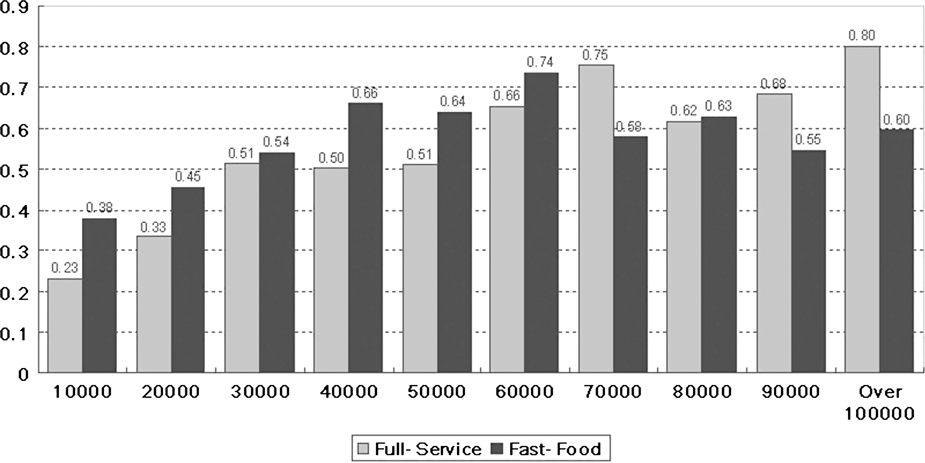
Number of table-service and fast-food restaurant visits. Values on Y-axis indicate frequency and X-axis indicates income.

Regressions with income squared and income alone on all-incomes samples

Table 2 presents regression results including the income squared variable for the full-service and fast-food all-incomes samples. The coefficients on income and income squared were statistically significant (P < 0.01) in both restaurant samples. The positive sign on income and negative sign on income squared implied inverted “U” curves. The coefficients implied that the frequency of full-service visits peaked at the income level of $95,000 and fast-food visits peaked at an income of $59,100. Because $95,000 was such a large number in our sample from the 1990s, the vast majority of respondents continued to visit full-service restaurants as incomes increased.

Table 2.

Frequency of Food Away from Home by Type of Eating Establishment: All Respondents

	Dependent Variables
	Number of full-service restaurant visits			Number of fast-food outlet visits
Independent Variables	Coefficient	P-value	IRR	Coefficient	P-value	IRR
Income	0.0155	(0.000)^***	1.016	0.013	(0.000)^***	1.013
Income Squared	−0.0000816	(0.014)^**	1.000	−0.00011	(0.001)^***	1.000
Age	0.016	(0.100)	1.016	−0.028	(0.002)^***	0.972
Age squared	0.000	(0.069)^*	1.000	0.000	(0.586)	1.000
Male	0.180	(0.001)^***	1.198	0.225	(0.000)^***	1.252
White	0.346	(0.001)^***	1.413	−0.232	(0.002)^***	0.793
Asian	0.444	(0.034)^**	1.559	−0.343	(0.076)^*	0.710
Other races	0.316	(0.058)^*	1.371	−0.011	(0.933)	0.989
Education	0.023	(0.033)^**	1.023	−0.002	(0.882)	0.998
Head	−0.153	(0.185)	0.858	−0.036	(0.702)	0.965
Household size	−0.117	(0.000)^***	0.890	−0.039	(0.024)^**	0.962
East	0.065	(0.413)	1.067	−0.099	(0.209)	0.906
Midwest	0.028	(0.708)	1.028	0.192	(0.006)^***	1.212
South	−0.041	(0.567)	0.960	0.238	(0.000)^***	1.269
Rural	−0.013	(0.842)	0.987	−0.215	(0.000)^***	0.807
Urban	0.090	(0.143)	1.094	−0.130	(0.018)^**	0.878
Food stamps	−0.350	(0.006)^***	0.704	0.055	(0.533)	1.056
Working hours	0.004	(0.001)^***	1.004	0.006	(0.000)^***	1.006
Obesity	0.100	(0.119)	1.106	0.077	(0.170)	1.080
TV	−0.092	(0.000)^***	0.912	−0.028	(0.017)^**	0.972
Exercise	0.068	(0.188)	1.070	−0.103	(0.026)^**	0.902
Smoking	−0.027	(0.661)	0.973	0.154	(0.003)^***	1.167
Drinking	0.089	(0.137)	1.093	−0.133	(0.011)^**	0.876
Friday	0.177	(0.001)^***	1.193	0.073	(0.141)	1.076
Saturday	0.018	(0.772)	1.018	0.050	(0.367)	1.051
Sunday	0.014	(0.799)	1.014	0.012	(0.808)	1.012
Price important	−0.158	(0.004)^***	0.854	−0.112	(0.022)^**	0.894
Convenience	0.124	(0.019)^**	1.132	0.111	(0.019)^**	1.118
Income level at which the frequency peaks	$95,000			$59,100

Single, double, and triple asterisks (^*) denote statistical significance at the 10%, 5%, and 1% levels, respectively.

Constant is not reported.

P values are in parentheses and based on robust standard error.

Income and income squared variables are in thousands.

The estimated coefficients and P values for income and income squared are not rounded for precise calculation.

Number of observations: 4972

For column 1: LR χ₂(28) = 414.51, corresponding to P < 0.01 for the overall significance of the regression. For column 2: LR χ₂(28) = 526.26, corresponding to P < 0.01 for the overall significance of the regression.

Men dined at both full-service and fast-food restaurants more frequently than women. Whites and Asians consumed more food at full-service restaurants, whereas African Americans consumed more fast food. Increased levels of education were associated only with increased full-service visits, not fast-food visits. As suggested by economies of scale in household food preparation,^9,10 visits to either type of restaurant decreased with household size (P < 0.01 for full service; P < 0.05 for fast food).

Regarding risk-related factors, we found that hours spent watching TV was negatively associated with full-service and fast-food restaurants. People who consume alcohol visited fast-food establishments less often than abstainers (P < 0.05), but people who smoke visited fast-food establishments more often than nonsmokers (P < 0.01). Exercise was significantly and negatively related to fast-food consumption (P < 0.05).

Consumers who consider price to be an important factor preferred to eat at home and eschewed both types of restaurants. However, consumers concerned with convenience visited both types of restaurants more often than consumers who were not concerned. Although all weekend variables are positively related with both types of eating establishments, only Friday is significantly related with full-service restaurant visits at the 5% confidence level.

To compare with earlier studies, we ran the same regressions with income but not income squared. The regression results in Table 3 show a statistically significant and positive association between income and full-service restaurant visits but a statistically insignificant association for fast food.

Table 3.

Frequency of food away from home without income squared

	Dependent Variables
Independent Variables	Number of full-service restaurant visits		Number of fast-food restaurant visits
Income	0.00585	(0.000)^***	0.00163	(0.134)

Triple asterisks (^*) denote statistical significance at the 1% level.

P values are in parentheses and based on robust standard error.

Income variable is in thousands.

The estimated coefficients and P values are not rounded for precise calculation.

All other coefficients are not shown but are available from the authors.

Number of observations: 4972

For column 1: LR χ₂(27) = 408.52, corresponding to P < 0.01 for the overall significance of the regression. For column 2: LR χ₂(27) = 513.63, corresponding to P < 0.01 for the overall significance of the regression.

Results from separate regressions by income level

Table 4 presents regression results for the below-average income group. Because our focus was on income, we make only 2 comments on other covariates. Within the below-average income group, education had a positive and statistically significant association with full-service visits (P < 0.05) but not fast-food visits. Interestingly, people who were obese and had below-average income dined out more frequently at full-service restaurants than their thinner counterparts. However, no obese/nonobese disparity was found for fast-food visits. The most important findings for us were that income was positively associated with visits to both types of restaurants for the below-average income group (P < 0.05) and the estimated income elasticity for full service (0.317) exceeded that for fast food (0.138). These elasticities imply that a 10% increase in income would be associated with 3.17% more visits to full-service restaurants and 1.38% more visits to fast-food restaurants.

Table 4.

Frequency of Visits by Type of Eating Establishment: Sample Below the Mean Income

	Dependent Variables
	Number of full-service restaurant visits			Number of fast-food outlet visits
Independent Variables	Coefficient	P value	IRR	Coefficient	P value	IRR
Log income	0.317	(0.000)^***	1.373	0.138	(0.024)^**	1.148
Age	0.010	(0.445)	1.010	−0.032	(0.005)^***	0.969
Age squared	0.000	(0.329)	1.000	0.000	(0.497)	1.000
Male	0.175	(0.027)^**	1.191	0.247	(0.000)^***	1.280
White	0.327	(0.016)^**	1.387	−0.220	(0.021)^**	0.803
Asian	0.791	(0.014)^**	2.206	−0.237	(0.439)	0.789
Other races	0.411	(0.050)^**	1.508	−0.013	(0.934)	0.987
Education	0.044	(0.004)^**	1.045	0.001	(0.926)	1.001
Head	0.153	(0.466)	1.165	0.010	(0.947)	1.010
Household size	−0.113	(0.001)^***	0.893	−0.070	(0.006)^***	0.933
East	0.031	(0.807)	1.031	−0.164	(0.166)	0.848
Midwest	0.007	(0.951)	1.007	0.229	(0.023)^**	1.257
South	−0.154	(0.161)	0.857	0.211	(0.025)^**	1.235
Rural	−0.048	(0.615)	0.953	−0.290	(0.000)^***	0.748
Urban	0.062	(0.513)	1.064	−0.201	(0.012)^**	0.818
Food stamps	−0.330	(0.026)^**	0.719	0.139	(0.165)	1.149
Working hours	0.004	(0.035)^**	1.004	0.005	(0.006)^***	1.005
Obesity	0.203	(0.035)^**	1.225	−0.007	(0.930)	0.993
TV	−0.105	(0.000)^***	0.901	−0.042	(0.005)^***	0.958
Exercise	0.101	(0.197)	1.107	−0.006	(0.933)	0.994
Smoking	0.108	(0.223)	1.114	0.184	(0.010)^***	1.202
Drinking	0.118	(0.168)	1.125	−0.176	(0.015)^**	0.839
Friday	0.102	(0.242)	1.107	0.085	(0.244)	1.088
Saturday	0.000	(0.999)	1.000	0.023	(0.781)	1.023
Sunday	0.032	(0.708)	1.033	−0.006	(0.932)	0.994
Price important	−0.117	(0.144)	0.889	−0.089	(0.192)	0.915
Convenience	0.161	(0.043)^**	1.175	0.134	(0.045)^**	1.144

Single, double, and triple asterisks (^*) denote statistical significance at the 10%, 5%, and 1% levels, respectively.

Constant is not reported.

P values are in parentheses and based on robust standard error.

N = 4972

For column 1: LR χ₂(27) = 207.33, corresponding to P < 0.01 for the overall significance of the regression. For column 2: LR χ₂(27) = 297.39, corresponding to P < 0.01 for the overall significance of the regression.

Regression results for the above-average income group are presented in Table 5. The most important results for us were that income was positively and statistically significantly associated with full-service visits (P < 0.01) but negatively and statistically significantly associated with fast-food visits (P < 0.05). In addition, people who were obese and had high incomes visited fast-food restaurants more frequently than their high-income, nonobese counterparts.

Table 5.

Frequency of Visits by Type of Eating Establishment: Sample Above the Mean Income

	Dependent Variables
	Number of full-service restaurant visits			Number of fast-food outlet visits
Independent Variables	Coefficient	P value	IRR	Coefficient	P value	IRR
Log income	0.375	(0.001)^***	1.454	−0.234	(0.030)^**	0.792
Age	0.019	(0.215)	1.019	0.007	(0.651)	1.007
Age squared	0.000	(0.232)	1.000	0.000	(0.053)^*	1.000
Male	0.170	(0.018)^**	1.185	0.189	(0.006)^***	1.208
White	0.311	(0.055)^*	1.365	−0.258	(0.026)^**	0.773
Asian	0.140	(0.626)	1.151	−0.442	(0.077)^*	0.643
Other races	0.068	(0.822)	1.070	0.035	(0.874)	1.035
Education	−0.014	(0.352)	0.986	−0.003	(0.834)	0.997
Head	−0.394	(0.005)^***	0.675	−0.125	(0.318)	0.883
Household size	−0.130	(0.000)^***	0.878	−0.013	(0.578)	0.987
East	0.098	(0.325)	1.103	−0.011	(0.914)	0.989
Midwest	0.044	(0.655)	1.045	0.146	(0.131)	1.157
South	0.081	(0.379)	1.085	0.296	(0.001)^***	1.345
Rural	0.063	(0.474)	1.065	−0.177	(0.041)^**	0.838
Urban	0.098	(0.211)	1.103	−0.046	(0.536)	0.955
Food stamps	0.337	(0.367)	1.401	0.145	(0.639)	1.156
Working hours	0.004	(0.036)^**	1.004	0.006	(0.000)^***	1.006
Obesity	0.016	(0.849)	1.017	0.188	(0.013)^**	1.207
TV	−0.081	(0.000)^***	0.922	0.004	(0.835)	1.004
Exercise	0.004	(0.956)	1.004	−0.180	(0.005)^***	0.835
Smoking	−0.203	(0.019)^**	0.816	0.089	(0.235)	1.093
Drinking	0.025	(0.767)	1.025	−0.073	(0.341)	0.929
Friday	0.248	(0.000)^***	1.282	0.061	(0.369)	1.063
Saturday	0.015	(0.853)	1.015	0.037	(0.623)	1.038
Sunday	−0.001	(0.992)	0.999	0.025	(0.721)	1.025
Price important	−0.183	(0.017)^**	0.833	−0.122	(0.083)^*	0.885
Convenience	0.090	(0.198)	1.094	0.082	(0.216)	1.085

Single, double, and triple asterisks (^*) denote statistical significance at the 10%, 5%, and 1% levels, respectively.

Constant is not reported.

P values are in parentheses and based on robust standard error.

N = 4972.

For column1: LR χ₂(27) = 120.81, corresponding to P < 0.01 for the overall significance of the regression. For column2: LR χ₂(27) = 230.1, corresponding to P < 0.01 for the overall significance of the regression.

Discussion

We found evidence for the Perloff hypothesis as it applies to full-service and fast-food restaurants. Full-service restaurants were “normal” for persons with high income (ie, persons with high levels of household income visited full-service restaurants more frequently than persons with low levels of income). Fast-food restaurants, on the other hand, were “normal” for persons with relatively low income, but were “inferior” for persons with relatively high income. These findings shed light on the ambiguous and statistically insignificant results from earlier studies^9,10 and our Table 3 that did not allow for varying visit or consumption patterns across income groups.

Our findings have implications for discussions of the causes of obesity. Many argue that a reason “poor” people have high prevalence of obesity is because they visit fast-food restaurants more frequently than “rich” people.^3,4 Our findings suggest that this is a simplistic argument. The relationship between income and fast-food visits is an inverted “U”, not a straight, downward-sloping line. Future fast-food research may need to be more careful when defining “poor” and “rich.” Moreover, visits to full-service restaurants, which also may serve large portions that contain much dietary fat, are more frequent among people with higher incomes than lower incomes.¹⁸ And as incomes increase, people may simply switch from fast-food to full-service restaurants. Finally, it might be that inexpensive, fat-dense, calorie-rich supermarket foods contribute most to obesity among those with the lowest incomes.

Earlier literature

Because, on average, meals at restaurants are more expensive than meals at home, economic theory suggests that restaurants should be “normal.” Previous studies have reported positive associations between household income and consumption of food away from home.^9,18

–22 However, the dependent variables in these studies are dollars spent, not visits. Spending as a dependent variable creates problems; higher spending may simply reflect higher prices. Our interest in obesity requires us to consider quantity, because it is quantity of food—not price—that may contribute to obesity. Furthermore, total household expenditures may depend especially on the size of household. Nevertheless, in a relevant study, McCracken and Brandt⁸ found positive and statistically significant associations between income and full-service spending, but insignificant associations for fast-food spending.

A limited number of studies investigate food intake rather than total expenditures. Studies by French et al⁴ and Jeffery and French³ report that frequency of fast-food restaurant use is higher among those with lower income and those who are nonwhite. However, the samples in both studies are not representative of the United States. Binkley¹⁰ uses a nationally representative sample and finds statistically significant, positive relationships between per capita income and full-service restaurant visits, but no statistical significance for fast-food visits.

Finally, our results are consistent with some obesity literature demonstrating racial differences. Earlier literature shows that African Americans are more likely to be obese than either whites or Asians, and our data show similar differences regarding visits to fast-food establishments.²³

Limitations

Our cross-sectional data cannot demonstrate causality. The high density of fast-food outlets in middle-income neighborhoods could be one explanation for the positive correlation between middle income and fast-food intake.^25
–27 The positive correlation might simply reflect the number of fast-food restaurants available rather than eating behaviors. But fast-food executives may have decided to locate resaturants in these neighborhoods precisely because they know the eating patterns of income groups.

An additional limitation involves the age of the data. We are unfamiliar with more recent data that contain the critical information on respondents' attitudes toward price and convenience. Finally, obesity and other behavioral variables are partly endogenous variables. In spite of this, those variables are included, mainly because they likely reduce unobservable heterogeneity and their introduction into the model causes little change in the main results.

In conclusion, our findings indicate that statistical relations between family income and restaurant visits are different between full service and fast food. For full-service restaurants, we find support for earlier studies: As incomes rise, so too do visits by individuals at all levels of income.⁹ For fast-food restaurants, earlier studies are flawed because they test only for either rising or falling consumption for all levels of income; they do not investigate whether an inverted “U” describes the relation.^9,10 We conclude that as incomes rise from the lowest levels to roughly the sample mean income, fast-food visits also rise; but as incomes rise beyond that threshold to the highest levels, fast-food visits fall. In the language of economics, full-service restaurants appear to be normal goods whereas fast-food restaurants appear to be normal up to a middle income value, but inferior for higher incomes.

Footnotes

Acknowledgment

Dr. Leigh acknowledges partial support from the National Institute for Occupational Safety and Health (Grant OH008248-01).

Author Disclosure Statement

Drs. Kim and Leigh disclosed no conflicts of interest.

References

Jeffery

, Baxter

, McGuire

, Linde

. Are fast food restaurants an environmental risk factor for obesity? Int J Behav Nutr Phys Act, 2006; 3:2.

Lin

, Guthrie

, Frazao

. Nutrient contribution of food away from home. Frazao

. America's Eating Habits: Changes and Consequences. http://www.ers.usda.gov/Publications/AIB750/. 2011 January 22.

Jeffery

, French

. Epidemic obesity in the United States: Are fast foods and television viewing contributing? Am J Public Health, 1998; 88:277–280.

French

, Harnack

, Jeffery

. Fast food restaurant use among women in the Pound of Prevention Study: Dietary, behavioral and demographic correlates. Int J Obes Metab Disord, 2000; 24:1353–1359.

Hill

, Wyatt

, Reed

, Peters

. Obesity and the environment: Where do we go from here? Science, 2003; 299:853–855.

Chou

, Grossman

, Saffer

. An economic analysis of adult obesity: Results from the Behavioral Risk Factor Surveillance System. J Health Econ, 2004; 23:565–587.

Pagan

, Davila

. Obesity, occupational attainment, and earnings. Soc Sci Q, 1997; 78:756–770.

Drewnowski

, Specter

. Poverty and obesity: The role of energy density and energy costs. Am J Clin Nutr, 2004; 79:6–16.

McCracken

, Brandt

. Household consumption of food-away-from-home: Total expenditure and by type of food facility. Am J Agric Econ, 1987; 69:274–284.

10.

Binkley

. The effect of demographic, economic, and nutrition factors on the frequency of food away from home. J Consumer Affairs, 2006; 40:372–391.

11.

Perloff

. Microeconomics. New York: Addison-Wesley, 2006.

12.

Tippett

, Cypel

. Design and Operation: The Continuing Survey of Food Intakes by Individuals and the Diet and Health Knowledge Survey 1994–96. Washington DC: US Dept of Agriculture, 1998.

13.

Bodner

, Perloff

. Databases for analyzing dietary data. The latest word from What We Eat in America. J Food Comp Anal, 2003; 16:347–358.

14.

Zhang

, Rashed

. Obesity and time preference: The health consequences of discounting the future. J Biosoc Sci, 2008; 40:97–113.

15.

Cameron

, Trivedi

. Regression Analysis of Count Data. New York: Cambridge University Press, 1998.

16.

Greene

. Accounting for Excess Zeros and Sample Selection in Poisson and Negative Binomial Regression Models. Working paper EC-94-10. New York: Stern School of Business, New York University, 1994.

17.

Leigh

, Folsom

. Estimates of value of accident-avoidance at the job depend on the concavity of the equalizing differences curve. Quart Rev Econ Bus, 1984; 24:56–66.

18.

Lin

, Frazao

. Nutritional quality of foods at and away from home. http://www.ers.usda.gov/publications/foodreview/aug1997/may97h.pdf. 2011 January 22.

19.

Cai

. Analyzing household food expenditure patterns on trips and vacations: A Tobit model. J Hosp Tourism Res, 1998; 22:338–358.

20.

Redman

. The impact of women's time allocation on expenditure for meals away from home and prepared foods. Am J Agric Econ, 1980; 62:234–237.

21.

Prochaska

, Schrimper

. Opportunity cost of time and other socioeconomic effects on away-from-home food consumption. Am J Agric Econ, 1973; 55:595–603.

22.

Soberon–Ferrer

, Dardis

. Determinants of household expenditures for services. J Consumer Res, 1991; 17:385–397.

23.

Ogden

, Carroll

, Curtin

, McDowell

, Tabak

, Flegal

. Prevalence of overweight and obesity in the United States, 1999–2004. JAMA, 2006; 295:1549–1555.

24.

Yen

. Working wives and food away from home: The Box–Cox Double Hurdle Model. Am J Agric Econ, 1993; 75:884–895.

25.

Block

, Scribner

, DeSalvo

. Fast food, race/ethnicity, and income: A geographic analysis. Am J Prev Med, 2004; 27:211–221.

26.

Reidpath

, Burns

, Garrard

, Mahoney

, Townsend

. An ecological study of the relationship between social and environmental determinants of obesity. Health Place, 2002; 8:141–145.

27.

Morland

, Wing

, Diez Roux

, Poole

. Neighborhood characteristics associated with the location of food stores and food service places. Am J Prev Med, 2002; 22:23–29.