Analyzing the Health Care Cost Curve: A Case Study

Background

Demographic factors play a large role in the level of spending by health insurers. In addition to cross-sectional differences in spending, health care spending tends to rise longitudinally. Spending for a 65-year-old male today tends to be more expensive than spending 10 years ago for an equivalent 65-year-old male. Models that assess how costs rise longitudinally for all, or most, groups are referred to as the “health care cost curve.” ¹

Actuarial models typically focus on PMPY or PMPM costs. This is a result of the managed care payer perspective. ² These frequencies of measurement are designed to conform to the way that actuaries measure, evaluate, and assess the cost of an insured population. For example, one important model of medical spending, forecast of the health care cost curve, comes from Medicare. Medicare collects aggregate figures for medical spending and breaks down the spending by payer and provider. Medicare also projects spending levels for 10 years based both on current law assumptions and reasonable alternative assumptions. The most recent estimate pegs medical spending at 17.9% of GDP in 2010, rising to 19.6% of GDP by 2021. ³ The major sources of uncertainty in the study include the effect of the Patient Protection and Affordable Care Act and the overall path of economic growth.

From the perspective of an insurance plan member, the health care cost curve is an annual phenomenon because plans assess and set the premiums once per year. From the insurer or employer's point of view, it could be a monthly phenomenon if costs steadily rise month by month. What is important to insurers is the effect of general inflation and spending trends on the growth in spending on insured services over time. However, according to a study by Bundorf et al, inflation alone is not sufficient to generate a cost curve because quantity changes are an important part of medical spending growth. ⁴ In the same study, the authors also note that studies of spending growth have generally focused on Medicare, and especially physician services within Medicare. Studies such as one by Sisko et al ⁵ have focused on the rate of growth in spending in the overall economy. These studies may help to determine trend assumptions for health insurance plans but are not population specific enough for many population health management applications.

Motivation

There is a lacuna in the literature that should be addressed by answering the question: With what frequency should the health care cost curve be measured? One way to demonstrate this gap is to look at how large databases of claims data have been analyzed in the past. Looking at publications resulting from the MarketScan data utilized in this study, no prior analysis has looked at the implications of analyzing health care spending at the daily level over the prior 15 years. ⁶ The reason that this question is important is that the frequency of measurement should be determined based on when interventions can be impactful. If the cost curve changes once per year, then disease management programs, plan renegotiations, and public policy need only be aimed at affecting the once yearly change in the level of spending. If the cost curve is continuously rising, then continuous process improvement may be the best policy. By determining the answer to the question of what the cost curve really looks like, this case study can inform efforts to bend the cost curve, maximizing the efficacy of such efforts.

To take a clinical example, a readmission prevention program may have interventions within 14 days of discharge with outcomes based on readmissions within a 30-day time horizon. ⁷ In this case, intervention could bend the cost curve up or down. Although the cost of these programs can be normed to a PMPM basis, this in a way obfuscates the true nature of the program because meaningful progress occurs daily. In this case, it may be necessary to measure costs on a daily basis, too. Such an analysis may offer an advantage over analyzing spending on a PMPY or PMPM basis. Although it is not necessary for clinical outcomes to perfectly match the horizon for financial outcomes, the measurement of outcomes should not be constrained by financial outcomes. In other words, the selection of clinical outcomes should not be dependent on the fact that financial data is available only annually or monthly.

From a statistical point of view, the frequency of measurement should maximize the chance of finding a statistically significant result. A pre/post design for studying any intervention may ignore a large degree of useful variation in outcomes of all kinds. It may be the case that real-time analysis is not currently possible for research, in that population health research cannot utilize hourly or real-time data. However, it is the case that practitioners have such a monitoring system as their ideal in many cases, as computing power and other technological improvements make continuous quality improvement a reality. Given that, the research methods utilized to study such programs also should be advanced toward a real-time analysis. There are several analyses that can potentially address these issues, such as an interrupted time series design. In the current study, a move from monthly to daily costs is investigated, which means the application of traditional (non-interrupted) time series designs to population health.

In general, episodes of care certainly do not follow neat monthly or yearly patterns. As a result, if the consumers of information about the health care cost curve are those in the field of population health management, then it is important to ask whether their needs are served by PMPY or PMPM calculations. If statistical analysis indicates that these models are obscuring important variation, then the result would be that population health management strategies with an aim of bending the cost curve would be underpowered, and therefore biased toward the null of no effect. Thus, it is important to find ways to determine what the statistical properties of the cost curve are in order to best design the protocols of population health management programs with a cost component.

Conceptual model

In reality, health care costs are incurred in real time. An investigation of health care costs that attempted to model costs over time, matching reality as closely as possible, would not divide the time line of care into discrete periods. Rather than chopping a period of time up into years, months, weeks, or days, such an analysis would model spending continuously over an entire time period as it actually happens. In finance, this is referred to as “continuous time,” as opposed to “discrete time,” modeling. ⁸ A closely related concept would be to use finer units of analysis: months as opposed to years, or days as opposed to months.

Consider the figures that show spending on an annual, monthly, and daily basis for a hypothetical plan (Fig. 1A and 1B). This plan has average annual costs per member that rise from $1000 at the beginning of 2000 to $2412 at the end of 2012. This represents a 7% compound annual growth rate in costs. Figure 1A shows what costs look like when viewed on a daily, monthly, and annual basis. Assuming that there is no variance around the trend line, the daily and monthly spending time series look very similar. From an analytic view, they are similar as well. Although the daily time series represents 4750 observations, the monthly time series represents 145 observations. Depending on the power of the study required, monthly data may be sufficient.

OPEN IN VIEWER

FIG. 1.

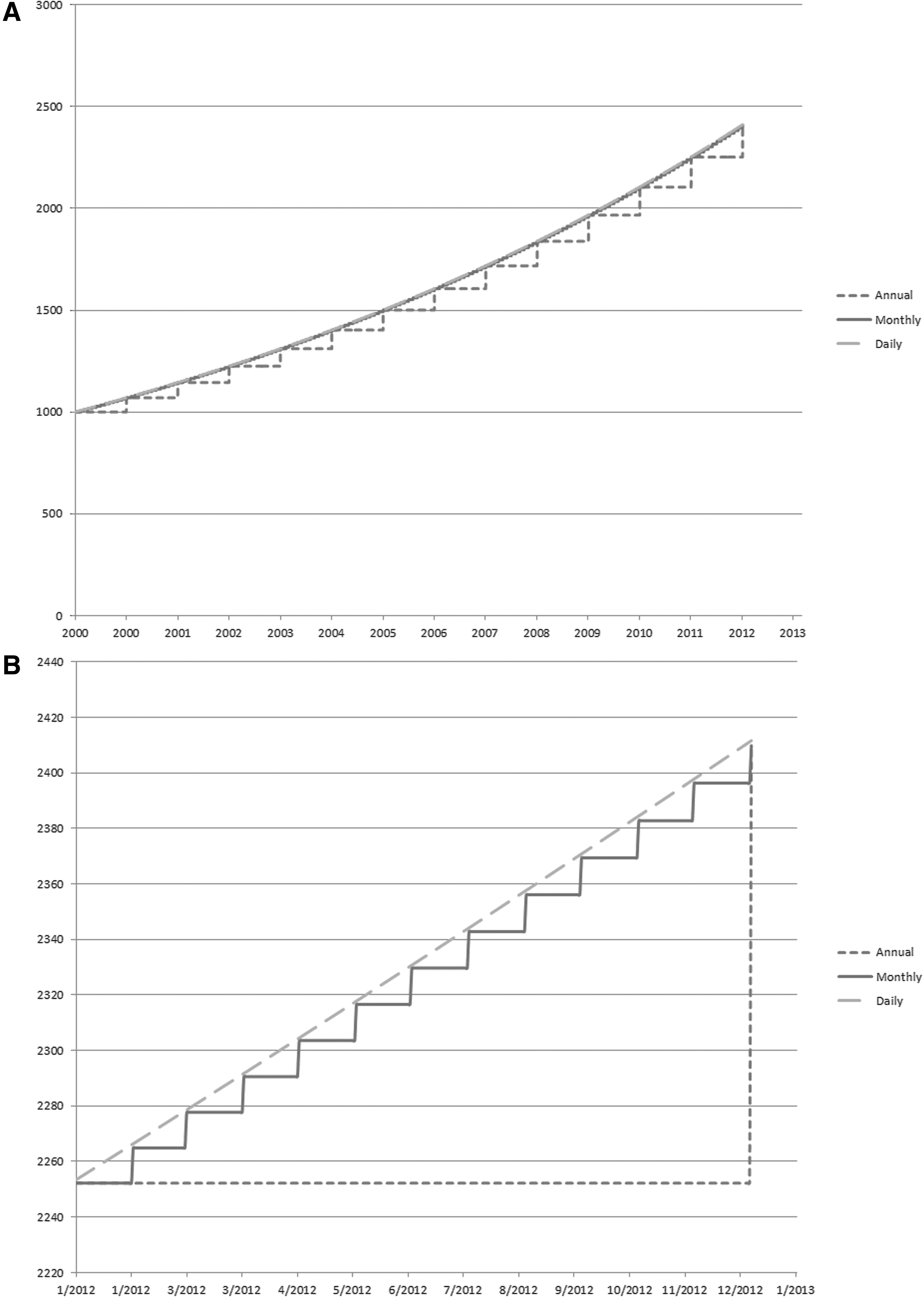
Conceptual model of annual, monthly, and daily spending.

Annual data may leave out a large degree of statistically important variation. There are a low number of observations—only 14. Thus, annualized data misrepresent reality to a significant extent. Such data understate costs for a large proportion of the year. This is not a statistical concern for some studies, for example, ones with a pre/post design or a long look back period. However, the annual spending model adversely affects a study with a shorter time horizon or the need for higher frequency monitoring. The performance of a treatment, program, or quality improvement initiative meant to decrease costs, is understated by such a model. The reason is that costs are constantly rising in the background because of reasons unrelated to the particular program. Thus, using annual or even monthly data will tend to bias study designs toward the null hypothesis that they have no effect on costs. For some managers, this type of measurement may be sufficient. For studies that require statistical significance in order to determine whether findings are positive, a bias toward the null is a detriment to the design of the best possible study.

Next, consider what costs would look like for a single year if costs grow continuously. This is presented in Figure 1B. In this case, daily data provide a superior view of actual cost trends than monthly or annual data. Daily data over the full year include 366 observations, while monthly data include 13 observations and annual data include 2 observations. PMPM analyses will tend to understate the effect of the program on bending the cost curve. These data are inadequate to support a study with multiple interventions, assessments of progress, and revised implementation throughout a single year.

The present study fit all 3 models to the data to determine which most accurately reflected reality. Did health care costs rise mainly on an annual basis, or is this a convenient unit of analysis for policy makers? Did health care costs rise on a monthly basis, or is this a convenient unit of analysis for managed care? Did health care costs rise on a daily basis?

Case study design

This study utilized a case study methodology in order to determine the characteristics of the health care cost curve for a population segmented by demographic factors. Taking advantage of a large database of employer-sponsored health insurance plans, the study prioritized several factors in considering which plans to include. The priorities were to find a large employer that was relatively stable, to find an employer that offered a single plan design, and to find an employer that reported both medical and drug costs. Out of 7 possible employers, a single large employer was chosen. Thus, the case study consisted of a population of continuously insured individuals who were salaried, nonunion workers (and their covered spouses) with a single insurance design. The cost curve was analyzed within this homogeneous sample.

Data

The MarketScan data utilized contained patient-level claims data for private insurers surveyed by the health care business of Thomson Reuters. ⁹ Thompson used the claims from the employers that submit data to create Health Insurance Portability and Accountability Act-compliant, limited-use data sets. The database was provided under a program of the National Bureau of Economic Research. The data files contained the reimbursements for inpatient, outpatient, and pharmaceutical encounters. The data files included population and enrollment files and benefit design files, as well as basic demographic information (age and sex). Geographic information, such as county and 3-digit zip code also were available, but were restricted to private use. There also was information on the total claim amount for any encounter and the split between the net amount paid by the plan and the amount paid by the employee.

The data selected from the database came from the health insurance plan of an anonymous employer in the Manufacturing, Nondurable Goods industry. Over the 7-year period of 2000–2006, only 1 plan was offered by this employer: a point-of-service (POS) plan with capitation. The employer's choice to offer only 1 type of plan, and not to change the plan offerings, allowed this study to isolate medical spending growth from other changes or plan switching behavior. This study did not control for changes in the benefit design because the composition of the basket of available medical care should change with changes in medical practice behavior. This study also did not control for the degree of capitation utilized in this POS plan or the variation in the type of capitation arrangement utilized over time.

The sample consisted of adults aged 18–64 years, who were covered as salaried, nonunion employees or the spouses of such employees. The sample only included individuals in a given year who were covered by the plan for the entire year. The total number of covered members varied year to year from 18–30 thousand members. Membership in the plan by sex within age group is shown in Table 1. The average population in the plan was 25,491, with no fewer than 18,000 in any given year. This study used the age groups defined in the MarketScan data (18–34, 35–44, 45–54, and 55–64). The population was virtually equally split between males and females, and larger for ages 18–34 and 35–44 than 45–54 and 55–64. Within age groups, only the oldest group, ages 55–64, ever had fewer than 1,000 members, with only 841 members in 2000. The split by sex was generally even, both overall and within age groups.

Expenditure data were available for encounters—drug fills, inpatient episodes, and outpatient visits. All files contained both the total payment made for each encounter, as well as the plan payment made by the insurer. The drug file includes more extensive information, including coinsurance, co-pays, and deductibles. The outpatient file included co-pays and deductibles in all years 2000–2006, but only included co-insurance beginning in 2005. The inpatient file only contained total and plan payments until 2005, when coinsurance, co-pay, and deductible payments also were recorded. All payments included dates of service and dates of payment, so date of service was used to allocate a claim amount to a claim date. Although the drug and outpatient experiences had a single service date attached to them, an inpatient episode could span multiple days. For that reason, the admission date was used when allocating inpatient expenses for an episode of care to a claim date.

Analysis

Disaggregating the cost curve by demographic group, this study compared and contrasted the spending growth rates of different groups, including which may be larger or more variable, and which were more predictable. A descriptive analysis was the first step to analyze the level of spending over time. This included an analysis of mean spending in total (insurance plan plus member spending) and plan spending alone per member per day. This spending was analyzed by year for plan years 2000–2006, and by month. Spending was compared on weekdays versus weekends, and by demographic groups including sex, age categories, and sex–age category subgroups. Age categories were defined in the MarketScan data (18–34, 35–44, 45–54, and 55–64).

A descriptive analysis of the growth in spending was the next step, in order to calculate and analyze the rate of change in spending over time. Both the rate of change in total spending and plan-only spending were analyzed. The average rate of change in spending PMPY, PMPM, and per member per day were computed. The analysis also was split by sex, age categories, and sex-age category subgroups. The rate of change in spending, or trend, was converted to a logarithmic basis. This also allowed the rate of change in spending to be modeled as a continuous time process. Thus, the rate of change in spending was calculated according to the following equation: \documentclass{aastex}\usepackage{amsbsy}\usepackage{amsfonts}\usepackage{amssymb}\usepackage{bm}\usepackage{mathrsfs}\usepackage{pifont}\usepackage{stmaryrd}\usepackage{textcomp}\usepackage{portland, xspace}\usepackage{amsmath, amsxtra}\pagestyle{empty}\DeclareMathSizes{10}{9}{7}{6}\begin{document} \begin{align*} \tau_{i , t} = \ln ( \hbox{Spending per capita}_{i, t} / \hbox{Spending per capita}_{i , t - 1} ) \\ \qquad\qquad\qquad \hbox{\rm For group }{i } \hbox{\rm for time }{ t } < { \rm Eq.} 1 > \end{align*} \end{document}

Equation 1: Log daily trend

Graphical analysis was applied as part of an exploratory modeling process to communicate what the results mean and to explore causes for the findings noted. Spending and encounter counts were explored for all claim types, and separately for drug fills, inpatient episodes, and outpatient visits. The differences in patterns between counts and spending were assessed to determine whether volume or prices could account for any results. Outpatient out-of-pocket payments were analyzed to determine the success of managed care payment techniques in managing and smoothing utilization. Although such analysis for all spending types would be ideal, only outpatient payments are available for the entire 2000–2006 period, which is a limitation of the data. Time series models were applied to remove noise in the data and to test the appropriateness of a continuous time model (additional detail available at http://jdc.jefferson.edu/healthpolicyfaculty/60/).

It was hypothesized that the health care cost curve would have a daily component as well as annual discontinuities. The daily component of health care spending is the time series modeled in Equation 1. The annual discontinuity would reflect the fact that managed care plans change benefit plans annually and renegotiate annually or every 2 to 3 years. As a result, there would be an annual “reset,” meaning a change in patient and provider behavior as they adjusted to the new plan design. This reset should have implications for health care costs, which could rise more or less in a given year depending on the success of managed care in holding down costs. Monthly discontinuities also were tested, with the hypothesis that because managed care finance is commonly managed on a monthly basis, there would be statistically significant differences in spending between months over the course of a year.

Once the final model was identified, it was fit to the data. The final model applied to generate the trend for group i for time t and the prediction error \documentclass{aastex}\usepackage{amsbsy}\usepackage{amsfonts}\usepackage{amssymb}\usepackage{bm}\usepackage{mathrsfs}\usepackage{pifont}\usepackage{stmaryrd}\usepackage{textcomp}\usepackage{portland, xspace}\usepackage{amsmath, amsxtra}\pagestyle{empty}\DeclareMathSizes{10}{9}{7}{6}\begin{document}$$\hat{e}_{i , t}$$ \end{document} was: \documentclass{aastex}\usepackage{amsbsy}\usepackage{amsfonts}\usepackage{amssymb}\usepackage{bm}\usepackage{mathrsfs}\usepackage{pifont}\usepackage{stmaryrd}\usepackage{textcomp}\usepackage{portland, xspace}\usepackage{amsmath, amsxtra}\pagestyle{empty}\DeclareMathSizes{10}{9}{7}{6}\begin{document} \begin{align*} \tau_{i , t} = \beta_0 + \beta_1 \cdot \tau_{i , t- 1} + \beta_2 \cdot \hbox{\rm Monday} + \beta_3 \cdot \hbox{\rm Saturday} \\ \hat{e}_{i , t} = \hat{\tau}_{i , t} - \tau_{i} < { \rm Eq.} 2 > \end{align*} \end{document}

Equation 2: Model for trend and error function

The coefficients of this model and the error terms were assessed to determine model goodness of fit and prediction error.

Level of spending

The per capita counts of encounters showed daily patterns but no clear trend over time. The inpatient counts were discrete, with few claims on any given day leading to “levels” in the graph of counts per capita by claim date and the histogram of counts. The drug and outpatient claims had 2, and possibly 3, different claim count levels corresponding to weekdays and weekends, with more claims on Saturday than Sunday. There was no discernible upward trend in encounters over the years, although there did appear to be a break in the trend in outpatient counts in 2003 (figures available from the author upon request). The overall count levels were mirrored in those of subgroups, such as males versus females. Thus, the count of encounters could not be used to account for the increased spending over time.

The age group categories defined in the data (18–34, 35–44, 45–54, and 55–64) and sex were used to break up the spending by demographic groups. Overall, each age group had significantly different spending even when compared to the closest (ie, the adjacent) age groups, with the older groups more expensive than the younger ones. The same was true within each year for total and plan spending. Separating weekdays from weekends, the difference remained only for weekday spending, suggesting that weekend spending, which is largely inpatient driven, is probably generated by emergencies that have nothing to do with age-related medical care. Spending was higher for females than males, and the difference between weekdays and weekends was more pronounced. These results in the levels confirmed the need to analyze medical trend by demographic group.

Medical trend

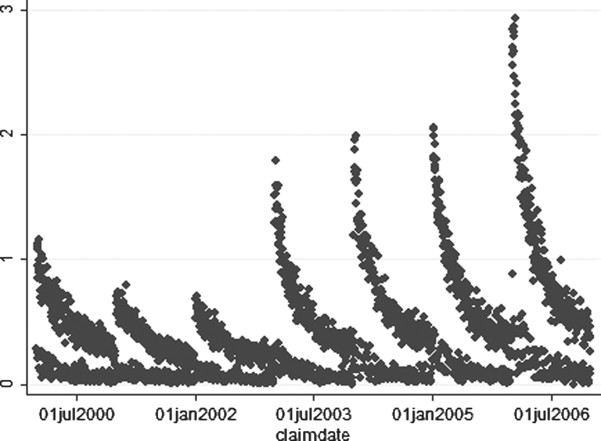
Total payments were rising both between and within years. Table 2 shows rising average nominal payments per member per day in each year, both overall and for the plan (net of member payments). Mean daily spending was statistically significantly different in each year. The average total spending (by plan and individuals) rose from $1926 in 2000 to $3740 in 2006, a 94% increase spread over 6 years. The corresponding compound annual growth rate was 11.7%, but the annual rates of change in mean spending ranged from 3% in 2003 to 16% in 2004. Plan spending increase was a nearly identical 93%, but this change masked even larger variation, including a 21% increase in 2002 and a 3% decrease in 2003. Figures 2 and 3 show the increase in spending over time for total spending and plan spending. The summarized results for the daily change in spending are in Table 3. The absolute value of average daily log change in spending by group was smaller than 0.001 in all cases. In some cases, the average was negative, but all figures are close to zero. However, the medians were all negative, whereas the skews were all positive, which is indicative of the fact that most spending growth was generated on a small number of days. The standard deviations were large enough that none of the means were indistinguishable from zero—on average, daily spending growth was zero. In addition, the standard deviation was lowest for the total population, smaller for younger than older ages, similar for males and females overall, and increasing by age groups for females, but not males. Thus, for purposes of analysis of average spending by demographic group, the total population had the most robust sample; younger groups had lower sampling error than older groups. The error rates may have been related to the size of the population sampled (Table 1). Additional results on model development are available at http://jdc.jefferson.edu/healthpolicyfaculty/60/.

OPEN IN VIEWER

FIG. 2.

Daily total spending per capita.

OPEN IN VIEWER

FIG. 3.

Daily plan spending per capita.

Graphical analysis confirmed the continuous increase in health care costs. Figure 2 shows this for total costs and Figure 3 shows a similar pattern for costs borne by the insurance plan alone. Both also exhibit a separation in spending, which was later confirmed as the weekday/weekend effect in the descriptive analysis. Finally, there was a great deal of noise in the data. It was possible to remove the seasonality or to fit 2 regression lines to the data. Ultimately, the choice was made to remove the seasonality and fit a single regression line (details available at http://jdc.jefferson.edu/healthpolicyfaculty/60/).

The final model chosen, presented in Equation 2 in the analysis section, contains only daily effects. The hypothesis that there is an annual component to the health care cost curve was not demonstrated in this study. There also were no monthly effects. Once the effects in daily spending were accounted for, month and year dummies were insignificant. As a result, managed care changes around benefit design and plan renegotiation did not show up in the cost curve of this case study as an annual “reset”; the growth in health care costs was continuous over the 7 years of the study.

An analysis of outpatient deductibles was performed as part of the analysis to determine why the health care cost curve was continuous in this case. The evidence strongly suggested that the annual reset in deductibles accounted for at least part of the effect. At the beginning of each year, patients pay high deductibles for care. As the year goes on, the graph suggests that patients start to reach their out-of-pocket limits, and deductibles actually paid fell toward zero before resetting (Fig. 4). This explanation could not be confirmed because of the anonymity involved in the MarketScan data. However, it is suggestive of the power of payment methods for smoothing utilization, and provided hypotheses to be explored further in future work.

OPEN IN VIEWER

FIG. 4.

Average outpatient deductible by day.

Goodness of fit

The power of the model to explain the variation in data varied across groups. The model accounted for approximately 70% of the variation in spending for all groups aggregated based on the adjusted R². The ability of the model to fit the cost curve varied from below 50% to above 60% in various age/sex categories. The lowest adjusted R² was for the youngest groups, despite the fact that the count of individuals was highest. This may have reflected the fact that, for the youngest group, spending growth is hardest to predict. For these groups, the predicted trend was farthest from the experienced trend, so they should receive particular scrutiny when quality improvement studies are performed.