Nonparametric Online Learning Control for Soft Continuum Robot: An Enabling Technique for Effective Endoscopic Navigation

Design of soft endoscope prototype

A generic, fluidic-driven soft continuum robot made of RTV (Room Temperature Vulcanization) silicone rubber (Ecoflex 0050; Smooth-On, Inc.) is designed and fabricated to evaluate the proposed framework for endoscopic navigation (Fig. 1a). The soft robot comprises three cylindrical inflatable chambers, each covered by a helical Kevlar string layer with a pitch of 1 mm. This fiber-constrained structure was first proposed by Suzumori et al.,^4,40 in which the helical constraint layer enforces axial anisotropic expansion of inflatable chambers so as to generate an effective bending moment when subject to pressure input. To enable effective endoscopic navigation, the three air chambers can be individually actuated by air or other fluid, facilitating a large panoramic workspace with a bending angle >150°. The slender robot configuration with 13-mm outer diameter and 93-mm length is also compatible with conventional endoscopes, which is of importance to dexterous manipulation inside a confined transluminal workspace.

OPEN IN VIEWER

FIG. 1.

(a) Soft robotic endoscope prototype made of silicone rubber. It has a dimension compatible with the insertion tube of conventional endoscope; (b) CAD/CAM model of the soft manipulator showing simulated helical strain-wrapping constrains around its individual actuation chamber using linear truss, where the anisotropic expansion can be achieved; (c) Finite element model tessellated with 12,000 linear hexahedron elements. A total of 2,214 truss elements are defined to emulate the effect of strain-wrapping constraint; (d) Cross-sectional area tessellated by hexahedron meshing.

Fabrication of the robot involves three major phases: (1) three cylindrical air chambers are cast with RTV silicone in inner molds; (2) Kevlar strings are wrapped densely in a single helical structure along each soft chamber; and (3) additional layers of silicone are cast to house the three inflatable chambers into one. This could fix the strings against dislocation, even after numerous bending actions.

Characterization of robot motion transition

Gradual smooth regulation of the fluidic flow rate allows steady bending of the presented soft manipulator. It also allows rapid reaching of fluid pressure equilibrium, minimizing the residual motion generated during such fluidic actuation. During endoscopic navigation within small and confined spaces (e.g., duodenum), such quasi-static motion characteristic ⁴¹ can facilitate effective precise targeting of the endoscopic camera or interventional tools (e.g., biopsy forceps or brush cytology) at the surgical regions of interest, thereby avoiding inadvertent damage to delicate tissue and potential discomfort to the patient.

To mathematically describe motion transition of the soft robot, let \documentclass{aastex}\usepackage{amsbsy}\usepackage{amsfonts}\usepackage{amssymb}\usepackage{bm}\usepackage{mathrsfs}\usepackage{pifont}\usepackage{stmaryrd}\usepackage{textcomp}\usepackage{portland, xspace}\usepackage{amsmath, amsxtra}\usepackage{upgreek}\pagestyle{empty}\DeclareMathSizes{10}{9}{7}{6}\begin{document} $${{ \bf{u}}_k} \in U$$ \end{document} be the fluid pressure (at equilibrium) in the actuation chambers at time step k where U denotes the control space. Let \documentclass{aastex}\usepackage{amsbsy}\usepackage{amsfonts}\usepackage{amssymb}\usepackage{bm}\usepackage{mathrsfs}\usepackage{pifont}\usepackage{stmaryrd}\usepackage{textcomp}\usepackage{portland, xspace}\usepackage{amsmath, amsxtra}\usepackage{upgreek}\pagestyle{empty}\DeclareMathSizes{10}{9}{7}{6}\begin{document} $${{ { \theta }}_k}$$ \end{document} be the state of the robot when the chambers are filled with the pressure of \documentclass{aastex}\usepackage{amsbsy}\usepackage{amsfonts}\usepackage{amssymb}\usepackage{bm}\usepackage{mathrsfs}\usepackage{pifont}\usepackage{stmaryrd}\usepackage{textcomp}\usepackage{portland, xspace}\usepackage{amsmath, amsxtra}\usepackage{upgreek}\pagestyle{empty}\DeclareMathSizes{10}{9}{7}{6}\begin{document} $${{ \bf{u}}_k}$$ \end{document} at equilibrium. This state corresponds to the distal tip position \documentclass{aastex}\usepackage{amsbsy}\usepackage{amsfonts}\usepackage{amssymb}\usepackage{bm}\usepackage{mathrsfs}\usepackage{pifont}\usepackage{stmaryrd}\usepackage{textcomp}\usepackage{portland, xspace}\usepackage{amsmath, amsxtra}\usepackage{upgreek}\pagestyle{empty}\DeclareMathSizes{10}{9}{7}{6}\begin{document} $${ \bf{p}} \in { \Re ^3}$$ \end{document} and orientation normal \documentclass{aastex}\usepackage{amsbsy}\usepackage{amsfonts}\usepackage{amssymb}\usepackage{bm}\usepackage{mathrsfs}\usepackage{pifont}\usepackage{stmaryrd}\usepackage{textcomp}\usepackage{portland, xspace}\usepackage{amsmath, amsxtra}\usepackage{upgreek}\pagestyle{empty}\DeclareMathSizes{10}{9}{7}{6}\begin{document} $${ \bf{n}} \in { \Re ^3}$$ \end{document} in the Cartesian space (Fig. 2), which are collectively represented by \documentclass{aastex}\usepackage{amsbsy}\usepackage{amsfonts}\usepackage{amssymb}\usepackage{bm}\usepackage{mathrsfs}\usepackage{pifont}\usepackage{stmaryrd}\usepackage{textcomp}\usepackage{portland, xspace}\usepackage{amsmath, amsxtra}\usepackage{upgreek}\pagestyle{empty}\DeclareMathSizes{10}{9}{7}{6}\begin{document} $${{ \bf{x}}_k} = { [ { \bf{p}} , { \bf{n}} ] ^T} \in { \Re ^6}$$ \end{document} . The forward transition model of the soft robot can be described by the following equation system: \documentclass{aastex}\usepackage{amsbsy}\usepackage{amsfonts}\usepackage{amssymb}\usepackage{bm}\usepackage{mathrsfs}\usepackage{pifont}\usepackage{stmaryrd}\usepackage{textcomp}\usepackage{portland, xspace}\usepackage{amsmath, amsxtra}\usepackage{upgreek}\pagestyle{empty}\DeclareMathSizes{10}{9}{7}{6}\begin{document} \begin{align*} \left\{ { \begin{matrix} {{{ { \theta }}_{k + 1}} = f ( {{ { \theta }}_k} , \Delta {{ \bf{u}}_k} ) } \\ {{{ \bf{x}}_k} = h ( {{{ \theta }}_k} ) } \\ \end{matrix} } \right. \tag{1} \end{align*} \end{document}

OPEN IN VIEWER

FIG. 2.

Three robot configurations illustrating an example of localized inverse models. Assume that their tip directions s _i will undergo the same rotation \documentclass{aastex}\usepackage{amsbsy}\usepackage{amsfonts}\usepackage{amssymb}\usepackage{bm}\usepackage{mathrsfs}\usepackage{pifont}\usepackage{stmaryrd}\usepackage{textcomp}\usepackage{portland, xspace}\usepackage{amsmath, amsxtra}\usepackage{upgreek}\pagestyle{empty}\DeclareMathSizes{10}{9}{7}{6}\begin{document} $$\Delta {{ \bf{s}}_{ref}}$$ \end{document} (blue arrow) when proper pressure changes \documentclass{aastex}\usepackage{amsbsy}\usepackage{amsfonts}\usepackage{amssymb}\usepackage{bm}\usepackage{mathrsfs}\usepackage{pifont}\usepackage{stmaryrd}\usepackage{textcomp}\usepackage{portland, xspace}\usepackage{amsmath, amsxtra}\usepackage{upgreek}\pagestyle{empty}\DeclareMathSizes{10}{9}{7}{6}\begin{document} $$\Delta {{ \bf{u}}_i}$$ \end{document} are applied, where \documentclass{aastex}\usepackage{amsbsy}\usepackage{amsfonts}\usepackage{amssymb}\usepackage{bm}\usepackage{mathrsfs}\usepackage{pifont}\usepackage{stmaryrd}\usepackage{textcomp}\usepackage{portland, xspace}\usepackage{amsmath, amsxtra}\usepackage{upgreek}\pagestyle{empty}\DeclareMathSizes{10}{9}{7}{6}\begin{document} $$i = 1 , 2 , 3$$ \end{document} . In the case of configurations 1 and 2, the average of their control inputs \documentclass{aastex}\usepackage{amsbsy}\usepackage{amsfonts}\usepackage{amssymb}\usepackage{bm}\usepackage{mathrsfs}\usepackage{pifont}\usepackage{stmaryrd}\usepackage{textcomp}\usepackage{portland, xspace}\usepackage{amsmath, amsxtra}\usepackage{upgreek}\pagestyle{empty}\DeclareMathSizes{10}{9}{7}{6}\begin{document} $$\Delta {{ \bf{u}}_1}$$ \end{document} and \documentclass{aastex}\usepackage{amsbsy}\usepackage{amsfonts}\usepackage{amssymb}\usepackage{bm}\usepackage{mathrsfs}\usepackage{pifont}\usepackage{stmaryrd}\usepackage{textcomp}\usepackage{portland, xspace}\usepackage{amsmath, amsxtra}\usepackage{upgreek}\pagestyle{empty}\DeclareMathSizes{10}{9}{7}{6}\begin{document} $$\Delta {{ \bf{u}}_2}$$ \end{document} would still lead to a rotation \documentclass{aastex}\usepackage{amsbsy}\usepackage{amsfonts}\usepackage{amssymb}\usepackage{bm}\usepackage{mathrsfs}\usepackage{pifont}\usepackage{stmaryrd}\usepackage{textcomp}\usepackage{portland, xspace}\usepackage{amsmath, amsxtra}\usepackage{upgreek}\pagestyle{empty}\DeclareMathSizes{10}{9}{7}{6}\begin{document} $$\Delta {{ \bf{s}}_{avg{ \rm{ }}1\& 2}}$$ \end{document} (red arrow) consistent with \documentclass{aastex}\usepackage{amsbsy}\usepackage{amsfonts}\usepackage{amssymb}\usepackage{bm}\usepackage{mathrsfs}\usepackage{pifont}\usepackage{stmaryrd}\usepackage{textcomp}\usepackage{portland, xspace}\usepackage{amsmath, amsxtra}\usepackage{upgreek}\pagestyle{empty}\DeclareMathSizes{10}{9}{7}{6}\begin{document} $$\Delta {{ \bf{s}}_{ref}}$$ \end{document} (blue arrow); When two configurations, such as 1 and 3, are vastly different, the average of inputs \documentclass{aastex}\usepackage{amsbsy}\usepackage{amsfonts}\usepackage{amssymb}\usepackage{bm}\usepackage{mathrsfs}\usepackage{pifont}\usepackage{stmaryrd}\usepackage{textcomp}\usepackage{portland, xspace}\usepackage{amsmath, amsxtra}\usepackage{upgreek}\pagestyle{empty}\DeclareMathSizes{10}{9}{7}{6}\begin{document} $$\Delta {{ \bf{u}}_1}$$ \end{document} and \documentclass{aastex}\usepackage{amsbsy}\usepackage{amsfonts}\usepackage{amssymb}\usepackage{bm}\usepackage{mathrsfs}\usepackage{pifont}\usepackage{stmaryrd}\usepackage{textcomp}\usepackage{portland, xspace}\usepackage{amsmath, amsxtra}\usepackage{upgreek}\pagestyle{empty}\DeclareMathSizes{10}{9}{7}{6}\begin{document} $$\Delta {{ \bf{u}}_3}$$ \end{document} may lead to a rotation \documentclass{aastex}\usepackage{amsbsy}\usepackage{amsfonts}\usepackage{amssymb}\usepackage{bm}\usepackage{mathrsfs}\usepackage{pifont}\usepackage{stmaryrd}\usepackage{textcomp}\usepackage{portland, xspace}\usepackage{amsmath, amsxtra}\usepackage{upgreek}\pagestyle{empty}\DeclareMathSizes{10}{9}{7}{6}\begin{document} $$\Delta {{ \bf{s}}_{avg{ \rm{ }}1\& 3}}$$ \end{document} (green arrow) that is significantly different from \documentclass{aastex}\usepackage{amsbsy}\usepackage{amsfonts}\usepackage{amssymb}\usepackage{bm}\usepackage{mathrsfs}\usepackage{pifont}\usepackage{stmaryrd}\usepackage{textcomp}\usepackage{portland, xspace}\usepackage{amsmath, amsxtra}\usepackage{upgreek}\pagestyle{empty}\DeclareMathSizes{10}{9}{7}{6}\begin{document} $$\Delta {{ \bf{s}}_{ref}}$$ \end{document} (blue arrow), leading to undesired movement. Therefore, learning the inverse model directly with a global function approximator may lead to invalid solutions and unstable robot performance.

where \documentclass{aastex}\usepackage{amsbsy}\usepackage{amsfonts}\usepackage{amssymb}\usepackage{bm}\usepackage{mathrsfs}\usepackage{pifont}\usepackage{stmaryrd}\usepackage{textcomp}\usepackage{portland, xspace}\usepackage{amsmath, amsxtra}\usepackage{upgreek}\pagestyle{empty}\DeclareMathSizes{10}{9}{7}{6}\begin{document} $$\Delta {{ \bf{u}}_k} = {{ \bf{u}}_{k + 1}} - {{ \bf{u}}_k}$$ \end{document} is the difference of the fluid pressure. The motion transition function f is a continuous mapping that depends on the current state of the robot \documentclass{aastex}\usepackage{amsbsy}\usepackage{amsfonts}\usepackage{amssymb}\usepackage{bm}\usepackage{mathrsfs}\usepackage{pifont}\usepackage{stmaryrd}\usepackage{textcomp}\usepackage{portland, xspace}\usepackage{amsmath, amsxtra}\usepackage{upgreek}\pagestyle{empty}\DeclareMathSizes{10}{9}{7}{6}\begin{document} $${{ { \theta }}_k}$$ \end{document} . Compared with rigid-link robots where the robot state can be well defined by joint kinematics, it is difficult to describe the exact state of the soft robot. For example, model-based approaches approximate this robot state based on PCC^{15,16,18,20–25} and non-PCC^26–30 constraints. The nonlinear function h transforms robot state \documentclass{aastex}\usepackage{amsbsy}\usepackage{amsfonts}\usepackage{amssymb}\usepackage{bm}\usepackage{mathrsfs}\usepackage{pifont}\usepackage{stmaryrd}\usepackage{textcomp}\usepackage{portland, xspace}\usepackage{amsmath, amsxtra}\usepackage{upgreek}\pagestyle{empty}\DeclareMathSizes{10}{9}{7}{6}\begin{document} $${{{ \theta }}_k}$$ \end{document} to Cartesian representation \documentclass{aastex}\usepackage{amsbsy}\usepackage{amsfonts}\usepackage{amssymb}\usepackage{bm}\usepackage{mathrsfs}\usepackage{pifont}\usepackage{stmaryrd}\usepackage{textcomp}\usepackage{portland, xspace}\usepackage{amsmath, amsxtra}\usepackage{upgreek}\pagestyle{empty}\DeclareMathSizes{10}{9}{7}{6}\begin{document} $${{ \bf{x}}_k}$$ \end{document} .

Typical endoscopic navigation requires delicate articulation of the distal tip so as to provide accurate positioning and easy access to the soft tissue lesion. A microcamera at the soft robot tip provides forward vision. Therefore, the operator can aim the distal tip at a lesion target on the luminal wall so as to guide the interventional instruments to deploy from the tip through the biopsy channel. This telemanipulated endoscopic navigation gives rise to a robot task space coordinate \documentclass{aastex}\usepackage{amsbsy}\usepackage{amsfonts}\usepackage{amssymb}\usepackage{bm}\usepackage{mathrsfs}\usepackage{pifont}\usepackage{stmaryrd}\usepackage{textcomp}\usepackage{portland, xspace}\usepackage{amsmath, amsxtra}\usepackage{upgreek}\pagestyle{empty}\DeclareMathSizes{10}{9}{7}{6}\begin{document} $${{ \bf{s}}_k}$$ \end{document} defined by its viewing direction (i.e., pitch and yaw angle). The system equation in Equation (1) can hence be extended to an actuation to task space mapping \documentclass{aastex}\usepackage{amsbsy}\usepackage{amsfonts}\usepackage{amssymb}\usepackage{bm}\usepackage{mathrsfs}\usepackage{pifont}\usepackage{stmaryrd}\usepackage{textcomp}\usepackage{portland, xspace}\usepackage{amsmath, amsxtra}\usepackage{upgreek}\pagestyle{empty}\DeclareMathSizes{10}{9}{7}{6}\begin{document} $${f_{ \bf{s}}}$$ \end{document} as follows: \documentclass{aastex}\usepackage{amsbsy}\usepackage{amsfonts}\usepackage{amssymb}\usepackage{bm}\usepackage{mathrsfs}\usepackage{pifont}\usepackage{stmaryrd}\usepackage{textcomp}\usepackage{portland, xspace}\usepackage{amsmath, amsxtra}\usepackage{upgreek}\pagestyle{empty}\DeclareMathSizes{10}{9}{7}{6}\begin{document} \begin{align*} {{ \bf{s}}_{k + 1}} = {f_{ \bf{s}}} ( {{{ \theta }}_k} , \Delta {{ \bf{u}}_k} ) \tag{2} \end{align*} \end{document}

where \documentclass{aastex}\usepackage{amsbsy}\usepackage{amsfonts}\usepackage{amssymb}\usepackage{bm}\usepackage{mathrsfs}\usepackage{pifont}\usepackage{stmaryrd}\usepackage{textcomp}\usepackage{portland, xspace}\usepackage{amsmath, amsxtra}\usepackage{upgreek}\pagestyle{empty}\DeclareMathSizes{10}{9}{7}{6}\begin{document} $${{ \bf{s}}_{k + 1}} = {{ \bf{s}}_k} + \Delta {{ \bf{s}}_k}$$ \end{document} is the task space coordinate at time step \documentclass{aastex}\usepackage{amsbsy}\usepackage{amsfonts}\usepackage{amssymb}\usepackage{bm}\usepackage{mathrsfs}\usepackage{pifont}\usepackage{stmaryrd}\usepackage{textcomp}\usepackage{portland, xspace}\usepackage{amsmath, amsxtra}\usepackage{upgreek}\pagestyle{empty}\DeclareMathSizes{10}{9}{7}{6}\begin{document} $$k + 1$$ \end{document} after the change in fluid pressure \documentclass{aastex}\usepackage{amsbsy}\usepackage{amsfonts}\usepackage{amssymb}\usepackage{bm}\usepackage{mathrsfs}\usepackage{pifont}\usepackage{stmaryrd}\usepackage{textcomp}\usepackage{portland, xspace}\usepackage{amsmath, amsxtra}\usepackage{upgreek}\pagestyle{empty}\DeclareMathSizes{10}{9}{7}{6}\begin{document} $$\Delta {{ \bf{u}}_k}$$ \end{document} is applied.

Inverse problem for online learning of task space control

Our control objective is to enable the operator to control displacement of the robot directly in the task space coordinate \documentclass{aastex}\usepackage{amsbsy}\usepackage{amsfonts}\usepackage{amssymb}\usepackage{bm}\usepackage{mathrsfs}\usepackage{pifont}\usepackage{stmaryrd}\usepackage{textcomp}\usepackage{portland, xspace}\usepackage{amsmath, amsxtra}\usepackage{upgreek}\pagestyle{empty}\DeclareMathSizes{10}{9}{7}{6}\begin{document} $$\Delta { \bf{s}}_k^*$$ \end{document} (i.e., the desired change in the robot tip orientation) with the use of a motion input device. The superscript “*” denotes the desired motion specified by users or other reference input. Thus, the controller is designed to approximate the inverse of the motion transition \documentclass{aastex}\usepackage{amsbsy}\usepackage{amsfonts}\usepackage{amssymb}\usepackage{bm}\usepackage{mathrsfs}\usepackage{pifont}\usepackage{stmaryrd}\usepackage{textcomp}\usepackage{portland, xspace}\usepackage{amsmath, amsxtra}\usepackage{upgreek}\pagestyle{empty}\DeclareMathSizes{10}{9}{7}{6}\begin{document} $${f_{ \bf{s}}}$$ \end{document} in Equation (2), that is, \documentclass{aastex}\usepackage{amsbsy}\usepackage{amsfonts}\usepackage{amssymb}\usepackage{bm}\usepackage{mathrsfs}\usepackage{pifont}\usepackage{stmaryrd}\usepackage{textcomp}\usepackage{portland, xspace}\usepackage{amsmath, amsxtra}\usepackage{upgreek}\pagestyle{empty}\DeclareMathSizes{10}{9}{7}{6}\begin{document} $$\Delta {{ \bf{u}}_k} = \tilde \Psi ( \Delta { \bf{s}}_k^* , {{{ \theta }}_k} )$$ \end{document} , to estimate the required change in control input \documentclass{aastex}\usepackage{amsbsy}\usepackage{amsfonts}\usepackage{amssymb}\usepackage{bm}\usepackage{mathrsfs}\usepackage{pifont}\usepackage{stmaryrd}\usepackage{textcomp}\usepackage{portland, xspace}\usepackage{amsmath, amsxtra}\usepackage{upgreek}\pagestyle{empty}\DeclareMathSizes{10}{9}{7}{6}\begin{document} $$\Delta {{ \bf{u}}_k}$$ \end{document} (as shown in Fig. 5). The inverse motion transition model \documentclass{aastex}\usepackage{amsbsy}\usepackage{amsfonts}\usepackage{amssymb}\usepackage{bm}\usepackage{mathrsfs}\usepackage{pifont}\usepackage{stmaryrd}\usepackage{textcomp}\usepackage{portland, xspace}\usepackage{amsmath, amsxtra}\usepackage{upgreek}\pagestyle{empty}\DeclareMathSizes{10}{9}{7}{6}\begin{document} $$\tilde \Psi$$ \end{document} heavily depends on the current robot state. However, the exact state \documentclass{aastex}\usepackage{amsbsy}\usepackage{amsfonts}\usepackage{amssymb}\usepackage{bm}\usepackage{mathrsfs}\usepackage{pifont}\usepackage{stmaryrd}\usepackage{textcomp}\usepackage{portland, xspace}\usepackage{amsmath, amsxtra}\usepackage{upgreek}\pagestyle{empty}\DeclareMathSizes{10}{9}{7}{6}\begin{document} $${{ { \theta }}_k}$$ \end{document} cannot be directly measured due to its hyperflexibility and the interactions with enclosed workspace inside a patient's cavity. We sought to adopt the task space coordinates \documentclass{aastex}\usepackage{amsbsy}\usepackage{amsfonts}\usepackage{amssymb}\usepackage{bm}\usepackage{mathrsfs}\usepackage{pifont}\usepackage{stmaryrd}\usepackage{textcomp}\usepackage{portland, xspace}\usepackage{amsmath, amsxtra}\usepackage{upgreek}\pagestyle{empty}\DeclareMathSizes{10}{9}{7}{6}\begin{document} $${ \bf{s}}$$ \end{document} , which would offer updated clues about the current robot state.

This approach is also of practical interest because these measurements are readily available in our control system. The task space coordinate \documentclass{aastex}\usepackage{amsbsy}\usepackage{amsfonts}\usepackage{amssymb}\usepackage{bm}\usepackage{mathrsfs}\usepackage{pifont}\usepackage{stmaryrd}\usepackage{textcomp}\usepackage{portland, xspace}\usepackage{amsmath, amsxtra}\usepackage{upgreek}\pagestyle{empty}\DeclareMathSizes{10}{9}{7}{6}\begin{document} $${ \bf{s}}$$ \end{document} can be tracked using advanced positional tracking systems. For example, electromagnetic (EM) tracking systems are commonly used in medical application to provide submillimeter-level tracking.^42,43 Together with the actuator's input \documentclass{aastex}\usepackage{amsbsy}\usepackage{amsfonts}\usepackage{amssymb}\usepackage{bm}\usepackage{mathrsfs}\usepackage{pifont}\usepackage{stmaryrd}\usepackage{textcomp}\usepackage{portland, xspace}\usepackage{amsmath, amsxtra}\usepackage{upgreek}\pagestyle{empty}\DeclareMathSizes{10}{9}{7}{6}\begin{document} $${{ \bf{u}}_k}$$ \end{document} , these online acquired data are presented to the learning algorithms to update the inverse mapping \documentclass{aastex}\usepackage{amsbsy}\usepackage{amsfonts}\usepackage{amssymb}\usepackage{bm}\usepackage{mathrsfs}\usepackage{pifont}\usepackage{stmaryrd}\usepackage{textcomp}\usepackage{portland, xspace}\usepackage{amsmath, amsxtra}\usepackage{upgreek}\pagestyle{empty}\DeclareMathSizes{10}{9}{7}{6}\begin{document} $$\Psi$$ \end{document} during robot run time. \documentclass{aastex}\usepackage{amsbsy}\usepackage{amsfonts}\usepackage{amssymb}\usepackage{bm}\usepackage{mathrsfs}\usepackage{pifont}\usepackage{stmaryrd}\usepackage{textcomp}\usepackage{portland, xspace}\usepackage{amsmath, amsxtra}\usepackage{upgreek}\pagestyle{empty}\DeclareMathSizes{10}{9}{7}{6}\begin{document} \begin{align*} \Delta {{ \bf{u}}_k} = \Psi ( \Delta { \bf{s}}_k^* , {{ \bf{s}}_k} , {{ \bf{u}}_k} ) \tag{3} \end{align*} \end{document}

Note that \documentclass{aastex}\usepackage{amsbsy}\usepackage{amsfonts}\usepackage{amssymb}\usepackage{bm}\usepackage{mathrsfs}\usepackage{pifont}\usepackage{stmaryrd}\usepackage{textcomp}\usepackage{portland, xspace}\usepackage{amsmath, amsxtra}\usepackage{upgreek}\pagestyle{empty}\DeclareMathSizes{10}{9}{7}{6}\begin{document} $$\Psi$$ \end{document} is the approximation of the true inverse mapping \documentclass{aastex}\usepackage{amsbsy}\usepackage{amsfonts}\usepackage{amssymb}\usepackage{bm}\usepackage{mathrsfs}\usepackage{pifont}\usepackage{stmaryrd}\usepackage{textcomp}\usepackage{portland, xspace}\usepackage{amsmath, amsxtra}\usepackage{upgreek}\pagestyle{empty}\DeclareMathSizes{10}{9}{7}{6}\begin{document} $$\tilde \Psi$$ \end{document} . If dimensionality of the task space is smaller than that of the control space, theoretically there exist an infinite number of solutions of \documentclass{aastex}\usepackage{amsbsy}\usepackage{amsfonts}\usepackage{amssymb}\usepackage{bm}\usepackage{mathrsfs}\usepackage{pifont}\usepackage{stmaryrd}\usepackage{textcomp}\usepackage{portland, xspace}\usepackage{amsmath, amsxtra}\usepackage{upgreek}\pagestyle{empty}\DeclareMathSizes{10}{9}{7}{6}\begin{document} $$\Delta {{ \bf{u}}_k}$$ \end{document} that result in the same task space displacement \documentclass{aastex}\usepackage{amsbsy}\usepackage{amsfonts}\usepackage{amssymb}\usepackage{bm}\usepackage{mathrsfs}\usepackage{pifont}\usepackage{stmaryrd}\usepackage{textcomp}\usepackage{portland, xspace}\usepackage{amsmath, amsxtra}\usepackage{upgreek}\pagestyle{empty}\DeclareMathSizes{10}{9}{7}{6}\begin{document} $$\Delta { \bf{s}}_k^*$$ \end{document} . This leads to the ill-posed problem in learning the inverse mapping \documentclass{aastex}\usepackage{amsbsy}\usepackage{amsfonts}\usepackage{amssymb}\usepackage{bm}\usepackage{mathrsfs}\usepackage{pifont}\usepackage{stmaryrd}\usepackage{textcomp}\usepackage{portland, xspace}\usepackage{amsmath, amsxtra}\usepackage{upgreek}\pagestyle{empty}\DeclareMathSizes{10}{9}{7}{6}\begin{document} $$\Psi$$ \end{document} .

Inverse model learning with multiple local controllers

Nonparametric local learning techniques have been applied to learn the ill-posed inverse problem, aiming to control redundantly actuated robots.^31,44,45 Referring to Peters and Schaal, ³⁶ the inverse model of a rigid-link robot can be learnt using spatially localized nonparametric learning techniques given that the robot state is well defined by joint kinematics. In this study, spatial localization refers to the robot state \documentclass{aastex}\usepackage{amsbsy}\usepackage{amsfonts}\usepackage{amssymb}\usepackage{bm}\usepackage{mathrsfs}\usepackage{pifont}\usepackage{stmaryrd}\usepackage{textcomp}\usepackage{portland, xspace}\usepackage{amsmath, amsxtra}\usepackage{upgreek}\pagestyle{empty}\DeclareMathSizes{10}{9}{7}{6}\begin{document} $${{ { \theta }}_k}$$ \end{document} . Such localization scheme is motivated by the hypothesis that the inverse problem would be well defined locally. ³⁶ It is because nonparametric learning techniques essentially average out the sampled data. Model learning based on nonconvex training datasets would give invalid solutions. ³⁶

However, in the vicinity of \documentclass{aastex}\usepackage{amsbsy}\usepackage{amsfonts}\usepackage{amssymb}\usepackage{bm}\usepackage{mathrsfs}\usepackage{pifont}\usepackage{stmaryrd}\usepackage{textcomp}\usepackage{portland, xspace}\usepackage{amsmath, amsxtra}\usepackage{upgreek}\pagestyle{empty}\DeclareMathSizes{10}{9}{7}{6}\begin{document} $$( { \bf{s}} , { \bf{u}} )$$ \end{document} , the average of \documentclass{aastex}\usepackage{amsbsy}\usepackage{amsfonts}\usepackage{amssymb}\usepackage{bm}\usepackage{mathrsfs}\usepackage{pifont}\usepackage{stmaryrd}\usepackage{textcomp}\usepackage{portland, xspace}\usepackage{amsmath, amsxtra}\usepackage{upgreek}\pagestyle{empty}\DeclareMathSizes{10}{9}{7}{6}\begin{document} $$\Delta { \bf{u}}$$ \end{document} would be consistent with the average of the task space displacement \documentclass{aastex}\usepackage{amsbsy}\usepackage{amsfonts}\usepackage{amssymb}\usepackage{bm}\usepackage{mathrsfs}\usepackage{pifont}\usepackage{stmaryrd}\usepackage{textcomp}\usepackage{portland, xspace}\usepackage{amsmath, amsxtra}\usepackage{upgreek}\pagestyle{empty}\DeclareMathSizes{10}{9}{7}{6}\begin{document} $$\Delta { \bf{s}}$$ \end{document} (Fig. 2). Therefore, in a local region of a given \documentclass{aastex}\usepackage{amsbsy}\usepackage{amsfonts}\usepackage{amssymb}\usepackage{bm}\usepackage{mathrsfs}\usepackage{pifont}\usepackage{stmaryrd}\usepackage{textcomp}\usepackage{portland, xspace}\usepackage{amsmath, amsxtra}\usepackage{upgreek}\pagestyle{empty}\DeclareMathSizes{10}{9}{7}{6}\begin{document} $$( { \bf{s}} , { \bf{u}} )$$ \end{document} , the training dataset \documentclass{aastex}\usepackage{amsbsy}\usepackage{amsfonts}\usepackage{amssymb}\usepackage{bm}\usepackage{mathrsfs}\usepackage{pifont}\usepackage{stmaryrd}\usepackage{textcomp}\usepackage{portland, xspace}\usepackage{amsmath, amsxtra}\usepackage{upgreek}\pagestyle{empty}\DeclareMathSizes{10}{9}{7}{6}\begin{document} $$\left\{ { \Delta { \bf{u}} , \Delta { \bf{s}} , { \bf{s}} , { \bf{u}}} \right\} $$ \end{document} would become a convex set. This enables learning of inverse mapping in the vicinity of \documentclass{aastex}\usepackage{amsbsy}\usepackage{amsfonts}\usepackage{amssymb}\usepackage{bm}\usepackage{mathrsfs}\usepackage{pifont}\usepackage{stmaryrd}\usepackage{textcomp}\usepackage{portland, xspace}\usepackage{amsmath, amsxtra}\usepackage{upgreek}\pagestyle{empty}\DeclareMathSizes{10}{9}{7}{6}\begin{document} $$( { \bf{s}} , { \bf{u}} )$$ \end{document} (Fig. 2). We approximate the local inverse mapping from the desired task space displacement to the actuation command as follows: \documentclass{aastex}\usepackage{amsbsy}\usepackage{amsfonts}\usepackage{amssymb}\usepackage{bm}\usepackage{mathrsfs}\usepackage{pifont}\usepackage{stmaryrd}\usepackage{textcomp}\usepackage{portland, xspace}\usepackage{amsmath, amsxtra}\usepackage{upgreek}\pagestyle{empty}\DeclareMathSizes{10}{9}{7}{6}\begin{document} \begin{align*} \Delta {{ \bf{u}}_k} = \Psi _{}^i ( \Delta { \bf{s}}_k^* , {{ \bf{s}}_k} , {{ \bf{u}}_k} ) = { [ \Delta { \bf{s}}_k^* ] ^{\rm T}}{ \beta ^i} \tag{4} \end{align*} \end{document}

where \documentclass{aastex}\usepackage{amsbsy}\usepackage{amsfonts}\usepackage{amssymb}\usepackage{bm}\usepackage{mathrsfs}\usepackage{pifont}\usepackage{stmaryrd}\usepackage{textcomp}\usepackage{portland, xspace}\usepackage{amsmath, amsxtra}\usepackage{upgreek}\pagestyle{empty}\DeclareMathSizes{10}{9}{7}{6}\begin{document} $${ \beta ^i}$$ \end{document} is the parameter of the local inverse model. Each mapping serves as a local controller. Compared with Peters et al., ³⁶ we do not include an intercept/bias term since the change of actuation command Δu should have zero mean. The computation of \documentclass{aastex}\usepackage{amsbsy}\usepackage{amsfonts}\usepackage{amssymb}\usepackage{bm}\usepackage{mathrsfs}\usepackage{pifont}\usepackage{stmaryrd}\usepackage{textcomp}\usepackage{portland, xspace}\usepackage{amsmath, amsxtra}\usepackage{upgreek}\pagestyle{empty}\DeclareMathSizes{10}{9}{7}{6}\begin{document} $${ \beta ^i}$$ \end{document} will be explained in the later context.

Online learning of the global controller

To approximate the global inverse mapping, we employ a linear combination of the locally learned mapping ⁴⁶ : \documentclass{aastex}\usepackage{amsbsy}\usepackage{amsfonts}\usepackage{amssymb}\usepackage{bm}\usepackage{mathrsfs}\usepackage{pifont}\usepackage{stmaryrd}\usepackage{textcomp}\usepackage{portland, xspace}\usepackage{amsmath, amsxtra}\usepackage{upgreek}\pagestyle{empty}\DeclareMathSizes{10}{9}{7}{6}\begin{document} \begin{align*} \begin{split}\Delta {{ \bf{u}}_k} = {{ \sum \nolimits_{i = 1}^n {{w^i} ( {{ \bf{s}}_k} , {{ \bf{u}}_k} ) \Phi _{}^i ( \Delta { \bf{s}}_k^* , {{ \bf{s}}_k} , {{ \bf{u}}_k} ) } } \over { \sum \nolimits_{i = 1}^n {{w^i} ( {{ \bf{s}}_k} , {{ \bf{u}}_k} ) } }} \\= {{ \sum \nolimits_{i = 1}^n {{w^i} ( {{ \bf{s}}_k} , {{ \bf{u}}_k} ) {{ [ \Delta { \bf{s}}_k^* ] }^T}{ \beta ^i}} } \over { \sum \nolimits_{i = 1}^n {{w^i} ( {{ \bf{s}}_k} , {{ \bf{u}}_k} ) } }}.\end{split} \tag{5} \end{align*} \end{document}

This controller architecture allows straightforward one-iteration computation in each time step, in contrast to indirect modeling approaches. ³⁴ The number of local models n and the weight \documentclass{aastex}\usepackage{amsbsy}\usepackage{amsfonts}\usepackage{amssymb}\usepackage{bm}\usepackage{mathrsfs}\usepackage{pifont}\usepackage{stmaryrd}\usepackage{textcomp}\usepackage{portland, xspace}\usepackage{amsmath, amsxtra}\usepackage{upgreek}\pagestyle{empty}\DeclareMathSizes{10}{9}{7}{6}\begin{document} $${w^i} ( {{ \bf{s}}_k} , {{ \bf{u}}_k} )$$ \end{document} , as well as the local controllers \documentclass{aastex}\usepackage{amsbsy}\usepackage{amsfonts}\usepackage{amssymb}\usepackage{bm}\usepackage{mathrsfs}\usepackage{pifont}\usepackage{stmaryrd}\usepackage{textcomp}\usepackage{portland, xspace}\usepackage{amsmath, amsxtra}\usepackage{upgreek}\pagestyle{empty}\DeclareMathSizes{10}{9}{7}{6}\begin{document} $$\Psi _{}^i ( \Delta { \bf{s}}_k^* , {{ \bf{s}}_k} , {{ \bf{u}}_k} )$$ \end{document} , can be obtained in an online manner.

For this purpose, the local forward model is learnt using locally weighted projection regression (LWPR), ³⁷ which offers piecewise linear function approximation, while it simultaneously determines the appropriate local region of each linear model. Each local forward model performs a linear mapping as follows: \documentclass{aastex}\usepackage{amsbsy}\usepackage{amsfonts}\usepackage{amssymb}\usepackage{bm}\usepackage{mathrsfs}\usepackage{pifont}\usepackage{stmaryrd}\usepackage{textcomp}\usepackage{portland, xspace}\usepackage{amsmath, amsxtra}\usepackage{upgreek}\pagestyle{empty}\DeclareMathSizes{10}{9}{7}{6}\begin{document} \begin{align*} \Delta { \bf{s}}_k^{} = f_{ \bf{s}}^i ( {{ \bf{s}}_k} , {{ \bf{u}}_k} , \Delta {{ \bf{u}}_k} ) = { [ \Delta {{ \bf{u}}_k} ] ^T}{ \hat \beta ^i} \tag{6} \end{align*} \end{document}

where \documentclass{aastex}\usepackage{amsbsy}\usepackage{amsfonts}\usepackage{amssymb}\usepackage{bm}\usepackage{mathrsfs}\usepackage{pifont}\usepackage{stmaryrd}\usepackage{textcomp}\usepackage{portland, xspace}\usepackage{amsmath, amsxtra}\usepackage{upgreek}\pagestyle{empty}\DeclareMathSizes{10}{9}{7}{6}\begin{document} $${ \hat \beta ^i}$$ \end{document} denotes the corresponding parameter. Each local region, namely the receptive field (RF), is shaped based on the membership function: \documentclass{aastex}\usepackage{amsbsy}\usepackage{amsfonts}\usepackage{amssymb}\usepackage{bm}\usepackage{mathrsfs}\usepackage{pifont}\usepackage{stmaryrd}\usepackage{textcomp}\usepackage{portland, xspace}\usepackage{amsmath, amsxtra}\usepackage{upgreek}\pagestyle{empty}\DeclareMathSizes{10}{9}{7}{6}\begin{document} \begin{align*} {w^i} ( {{ \bf{s}}_k} , {{ \bf{u}}_k} ) = \exp \left( { - 0.5{{ \left( { \left[ { \begin{matrix} {{{ \bf{s}}_k}} \\ {{{ \bf{u}}_k}} \\ \end{matrix} } \right] - {{ \bf{c}}^i}} \right) }^{\rm T}}{{ \bf{D}}^i} \left( { \left[ { \begin{matrix} {{{ \bf{s}}_k}} \\ {{{ \bf{u}}_k}} \\ \end{matrix} } \right] - {{ \bf{c}}^i}} \right) } \right) \tag{7} \end{align*} \end{document}

centered at \documentclass{aastex}\usepackage{amsbsy}\usepackage{amsfonts}\usepackage{amssymb}\usepackage{bm}\usepackage{mathrsfs}\usepackage{pifont}\usepackage{stmaryrd}\usepackage{textcomp}\usepackage{portland, xspace}\usepackage{amsmath, amsxtra}\usepackage{upgreek}\pagestyle{empty}\DeclareMathSizes{10}{9}{7}{6}\begin{document} $${{ \bf{c}}^i}$$ \end{document} , where D ⁱ is the distance metric. Each membership function weights the corresponding locally learned inverse model in the controller (Eq. 6).

One advantage of LWPR is that it can automatically spawn new linear models and the corresponding RF when new data laid outside all existing RF are presented. Meanwhile, the center \documentclass{aastex}\usepackage{amsbsy}\usepackage{amsfonts}\usepackage{amssymb}\usepackage{bm}\usepackage{mathrsfs}\usepackage{pifont}\usepackage{stmaryrd}\usepackage{textcomp}\usepackage{portland, xspace}\usepackage{amsmath, amsxtra}\usepackage{upgreek}\pagestyle{empty}\DeclareMathSizes{10}{9}{7}{6}\begin{document} $${{ \bf{c}}^i}$$ \end{document} of RF is determined by the input space of new data through incremental learning so as the total number of local regions n (Fig. 3). Each newly spawned RF is initialized with a diagonal distance metric D ⁱ value. This D ⁱ value will be updated throughout the incremental learning process to improve the overall regression accuracy and convergence rate. To prevent overfitting and allocation of too many numbers of RFs n, a smaller initial D ⁱ value is preferred (i.e., larger RFs). Cross-validation is also employed in determining the initial D ⁱ , which is important to ensure that the forward model can be accurately reflected by piecewise linear regression.

OPEN IN VIEWER

FIG. 3.

Example set of localized linear controllers that approximate the nonlinear inverse mapping \documentclass{aastex}\usepackage{amsbsy}\usepackage{amsfonts}\usepackage{amssymb}\usepackage{bm}\usepackage{mathrsfs}\usepackage{pifont}\usepackage{stmaryrd}\usepackage{textcomp}\usepackage{portland, xspace}\usepackage{amsmath, amsxtra}\usepackage{upgreek}\pagestyle{empty}\DeclareMathSizes{10}{9}{7}{6}\begin{document} $$\Psi$$ \end{document} of a 1D actuation \documentclass{aastex}\usepackage{amsbsy}\usepackage{amsfonts}\usepackage{amssymb}\usepackage{bm}\usepackage{mathrsfs}\usepackage{pifont}\usepackage{stmaryrd}\usepackage{textcomp}\usepackage{portland, xspace}\usepackage{amsmath, amsxtra}\usepackage{upgreek}\pagestyle{empty}\DeclareMathSizes{10}{9}{7}{6}\begin{document} $$\Delta { \bf{u}}$$ \end{document} . The valid region of each spatially localized controller is centered at \documentclass{aastex}\usepackage{amsbsy}\usepackage{amsfonts}\usepackage{amssymb}\usepackage{bm}\usepackage{mathrsfs}\usepackage{pifont}\usepackage{stmaryrd}\usepackage{textcomp}\usepackage{portland, xspace}\usepackage{amsmath, amsxtra}\usepackage{upgreek}\pagestyle{empty}\DeclareMathSizes{10}{9}{7}{6}\begin{document} $${{ \bf{c}}^i}$$ \end{document} (denoted by plus sign), with the range parameterized by \documentclass{aastex}\usepackage{amsbsy}\usepackage{amsfonts}\usepackage{amssymb}\usepackage{bm}\usepackage{mathrsfs}\usepackage{pifont}\usepackage{stmaryrd}\usepackage{textcomp}\usepackage{portland, xspace}\usepackage{amsmath, amsxtra}\usepackage{upgreek}\pagestyle{empty}\DeclareMathSizes{10}{9}{7}{6}\begin{document} $${{ \bf{D}}^i}$$ \end{document} (colored ellipse) in the robot state space. The warm color depicts the actuation \documentclass{aastex}\usepackage{amsbsy}\usepackage{amsfonts}\usepackage{amssymb}\usepackage{bm}\usepackage{mathrsfs}\usepackage{pifont}\usepackage{stmaryrd}\usepackage{textcomp}\usepackage{portland, xspace}\usepackage{amsmath, amsxtra}\usepackage{upgreek}\pagestyle{empty}\DeclareMathSizes{10}{9}{7}{6}\begin{document} $$\Delta { \bf{u}}$$ \end{document} predicted by the linear control law \documentclass{aastex}\usepackage{amsbsy}\usepackage{amsfonts}\usepackage{amssymb}\usepackage{bm}\usepackage{mathrsfs}\usepackage{pifont}\usepackage{stmaryrd}\usepackage{textcomp}\usepackage{portland, xspace}\usepackage{amsmath, amsxtra}\usepackage{upgreek}\pagestyle{empty}\DeclareMathSizes{10}{9}{7}{6}\begin{document} $${ \beta ^i}$$ \end{document} to achieve a particular movement \documentclass{aastex}\usepackage{amsbsy}\usepackage{amsfonts}\usepackage{amssymb}\usepackage{bm}\usepackage{mathrsfs}\usepackage{pifont}\usepackage{stmaryrd}\usepackage{textcomp}\usepackage{portland, xspace}\usepackage{amsmath, amsxtra}\usepackage{upgreek}\pagestyle{empty}\DeclareMathSizes{10}{9}{7}{6}\begin{document} $$\Delta { \bf{s}}_{}^*$$ \end{document} in task space.

Despite the fact that each RF could fulfill the local convexity requirement due to redundancy in the robotic system, the solutions of local controllers (Eq. 4) could be inconsistent with the desired solutions. ³⁶ Although this problem could be resolved by preprocessing the training data such that it only produces one particular solution, it lacks generality and is difficult to apply in high-dimensional systems. ³¹ Therefore, we employ another approach that reshapes local inverse models using constrained optimization, where the local controllers are enforced to provide consistent solutions from infinite possibilities in the null space of the control space. We then define the optimization problem as follows: \documentclass{aastex}\usepackage{amsbsy}\usepackage{amsfonts}\usepackage{amssymb}\usepackage{bm}\usepackage{mathrsfs}\usepackage{pifont}\usepackage{stmaryrd}\usepackage{textcomp}\usepackage{portland, xspace}\usepackage{amsmath, amsxtra}\usepackage{upgreek}\pagestyle{empty}\DeclareMathSizes{10}{9}{7}{6}\begin{document} \begin{align*} \mathop { \min } \limits_{ \Delta { \bf{u}}} {C_k} ( \Delta {{ \bf{u}}_k} ) = { ( \Delta {{ \bf{u}}_k} - \Delta {{ \bf{u}}_{0 , k}} ) ^{\rm T}}{ \bf{N}} ( \Delta {{ \bf{u}}_k} - \Delta {{ \bf{u}}_{0 , k}} ) \tag{8} \end{align*} \end{document}

subject to \documentclass{aastex}\usepackage{amsbsy}\usepackage{amsfonts}\usepackage{amssymb}\usepackage{bm}\usepackage{mathrsfs}\usepackage{pifont}\usepackage{stmaryrd}\usepackage{textcomp}\usepackage{portland, xspace}\usepackage{amsmath, amsxtra}\usepackage{upgreek}\pagestyle{empty}\DeclareMathSizes{10}{9}{7}{6}\begin{document} $$\Delta {{ \bf{u}}_k} = \Psi ( \Delta { \bf{s}}_k^* , {{ \bf{s}}_k} , {{ \bf{u}}_k} )$$ \end{document}

where the cost function C_k represents the user-defined optimality scaled by a diagonal matrix N. \documentclass{aastex}\usepackage{amsbsy}\usepackage{amsfonts}\usepackage{amssymb}\usepackage{bm}\usepackage{mathrsfs}\usepackage{pifont}\usepackage{stmaryrd}\usepackage{textcomp}\usepackage{portland, xspace}\usepackage{amsmath, amsxtra}\usepackage{upgreek}\pagestyle{empty}\DeclareMathSizes{10}{9}{7}{6}\begin{document} $$\Delta {{ \bf{u}}_{0 , k}} = \upsilon ( {{ \bf{s}}_k} , {{ \bf{u}}_k} )$$ \end{document} is the user-defined null-space behavior. One example of null-space behavior could be minimizing the elongation of the robot, which results in smaller bending radius to facilitate dexterous motion inside enclosed cavity. Finally, the optimization constraint \documentclass{aastex}\usepackage{amsbsy}\usepackage{amsfonts}\usepackage{amssymb}\usepackage{bm}\usepackage{mathrsfs}\usepackage{pifont}\usepackage{stmaryrd}\usepackage{textcomp}\usepackage{portland, xspace}\usepackage{amsmath, amsxtra}\usepackage{upgreek}\pagestyle{empty}\DeclareMathSizes{10}{9}{7}{6}\begin{document} $$\Delta {{ \bf{u}}_k} = \Psi ( \Delta { \bf{s}}_k^* , {{ \bf{s}}_k} , {{ \bf{u}}_k} )$$ \end{document} ensures the correctness of the inverse solution.

The constrained optimization problem can be solved by introducing a reward function (Eq. 9) and a cost function (Eq. 10): \documentclass{aastex}\usepackage{amsbsy}\usepackage{amsfonts}\usepackage{amssymb}\usepackage{bm}\usepackage{mathrsfs}\usepackage{pifont}\usepackage{stmaryrd}\usepackage{textcomp}\usepackage{portland, xspace}\usepackage{amsmath, amsxtra}\usepackage{upgreek}\pagestyle{empty}\DeclareMathSizes{10}{9}{7}{6}\begin{document} \begin{align*} r ( {{ \bf{u}}_k} ) = { \sigma _i} \exp ( - 0.5 \sigma _i^2{C_k} ) \tag{9} \end{align*} \end{document} \documentclass{aastex}\usepackage{amsbsy}\usepackage{amsfonts}\usepackage{amssymb}\usepackage{bm}\usepackage{mathrsfs}\usepackage{pifont}\usepackage{stmaryrd}\usepackage{textcomp}\usepackage{portland, xspace}\usepackage{amsmath, amsxtra}\usepackage{upgreek}\pagestyle{empty}\DeclareMathSizes{10}{9}{7}{6}\begin{document} \begin{align*} {E_i} = \mathop \sum \limits_{k = 1}^N {r ( {{ \bf{u}}_k} ) {w^i} ( {{ \bf{s}}_k} , {{ \bf{u}}_k} ) {{ ( \Delta {{ \bf{u}}_k} - [ \Delta { \bf{s}}_k^T ] {{ { \beta }}^i} ) }^2}} \tag{10} \end{align*} \end{document}

The reward function \documentclass{aastex}\usepackage{amsbsy}\usepackage{amsfonts}\usepackage{amssymb}\usepackage{bm}\usepackage{mathrsfs}\usepackage{pifont}\usepackage{stmaryrd}\usepackage{textcomp}\usepackage{portland, xspace}\usepackage{amsmath, amsxtra}\usepackage{upgreek}\pagestyle{empty}\DeclareMathSizes{10}{9}{7}{6}\begin{document} $$r ( {{ \bf{u}}_k} )$$ \end{document} is scaled by the mean cost \documentclass{aastex}\usepackage{amsbsy}\usepackage{amsfonts}\usepackage{amssymb}\usepackage{bm}\usepackage{mathrsfs}\usepackage{pifont}\usepackage{stmaryrd}\usepackage{textcomp}\usepackage{portland, xspace}\usepackage{amsmath, amsxtra}\usepackage{upgreek}\pagestyle{empty}\DeclareMathSizes{10}{9}{7}{6}\begin{document} $${ \sigma _i}$$ \end{document} to improve learning efficiency ³⁶ : \documentclass{aastex}\usepackage{amsbsy}\usepackage{amsfonts}\usepackage{amssymb}\usepackage{bm}\usepackage{mathrsfs}\usepackage{pifont}\usepackage{stmaryrd}\usepackage{textcomp}\usepackage{portland, xspace}\usepackage{amsmath, amsxtra}\usepackage{upgreek}\pagestyle{empty}\DeclareMathSizes{10}{9}{7}{6}\begin{document} \begin{align*} \sigma _i^2 = \sum \nolimits_{h = 1}^k {{w^i} ( {{ \bf{s}}_h} , {{ \bf{u}}_h} ) } {C_h} / \sum \nolimits_{h = 1}^k {{w^i} ( {{ \bf{s}}_h} , {{ \bf{u}}_h} ) } \tag{11} \end{align*} \end{document}

The cost function is then minimized by means of reward-weighted regression, where each local model needed to be updated: \documentclass{aastex}\usepackage{amsbsy}\usepackage{amsfonts}\usepackage{amssymb}\usepackage{bm}\usepackage{mathrsfs}\usepackage{pifont}\usepackage{stmaryrd}\usepackage{textcomp}\usepackage{portland, xspace}\usepackage{amsmath, amsxtra}\usepackage{upgreek}\pagestyle{empty}\DeclareMathSizes{10}{9}{7}{6}\begin{document} \begin{align*} {{ \beta }}_{k + 1}^i = { ( {{ \bf{X}}^{\rm T}}{{ \bf{W}}^i}{ \bf{X}} ) ^{ - 1}}{{ \bf{X}}^T}{{ \bf{W}}^i}{ \bf{Y}} \tag{12} \end{align*} \end{document}

where \documentclass{aastex}\usepackage{amsbsy}\usepackage{amsfonts}\usepackage{amssymb}\usepackage{bm}\usepackage{mathrsfs}\usepackage{pifont}\usepackage{stmaryrd}\usepackage{textcomp}\usepackage{portland, xspace}\usepackage{amsmath, amsxtra}\usepackage{upgreek}\pagestyle{empty}\DeclareMathSizes{10}{9}{7}{6}\begin{document} $${{ \bf{W}}^i} = diag ( r ( {{ \bf{u}}_1} ) w_1^i , \, \ldots \, , r ( {{ \bf{u}}_k} ) w_k^i )$$ \end{document} , \documentclass{aastex}\usepackage{amsbsy}\usepackage{amsfonts}\usepackage{amssymb}\usepackage{bm}\usepackage{mathrsfs}\usepackage{pifont}\usepackage{stmaryrd}\usepackage{textcomp}\usepackage{portland, xspace}\usepackage{amsmath, amsxtra}\usepackage{upgreek}\pagestyle{empty}\DeclareMathSizes{10}{9}{7}{6}\begin{document} $${ \bf{X}} = [ \Delta { \bf{s}}_k^* ]$$ \end{document} , and \documentclass{aastex}\usepackage{amsbsy}\usepackage{amsfonts}\usepackage{amssymb}\usepackage{bm}\usepackage{mathrsfs}\usepackage{pifont}\usepackage{stmaryrd}\usepackage{textcomp}\usepackage{portland, xspace}\usepackage{amsmath, amsxtra}\usepackage{upgreek}\pagestyle{empty}\DeclareMathSizes{10}{9}{7}{6}\begin{document} $${ \bf{Y}} = [ \Delta {{ \bf{u}}_k} ]$$ \end{document} are the training datasets. The overall procedures of the learning-based controller are summarized in Algorithm 1.

Initialization of online learning by FEA-based model

Proper initialization of pretraining data is essential to many online learning techniques. These preceding data are dedicated to pretraining an initial control policy before the online learning begins. It is usually acquired by driving the robot with random input. Instead, we proposed to incorporate FEA, by which robot deformation can be simulated with a hyperelastic computation model. This simulation can generate comprehensive pretraining samples that cover the entire robot workspace at a high resolution, facilitating offline pretraining of the learning-based controller (Fig. 5).

The FEA model of the robot is constructed using ABAQUS ⁴⁷ to predict the robot kinematics and workspace. RTV silicone rubber is considered as incompressible hyperelastic material formulated by Odgen material model. ⁴⁸ It exhibits negligible volume change under hydrostatic compression and has a Poisson's ratio close to 0.5. Due to the incompressibility of silicone rubber and the large deformation nature of the simulation, the element formulation and mesh quality pose a compelling effect on both accuracy and convergence of the simulation. Therefore, hexahedral element (C3D8RH; Fig. 1c) based on u-p hybrid formulation with hourglass control ⁴⁷ is chosen over the commonly used quadratic tetrahedral elements (Fig. 1d) in the FEA of our soft robotic manipulators.

The C3D8RH element possesses eight displacement nodes and one interior pressure node. The combination of these displacement and pressure nodes is often close to optimal. ⁴⁹ Such integration scheme improves not only element efficiency but also element accuracy under bending load. However, compared with tetrahedrons, automatic mesh generation of hexahedrons is relatively ineffective, resulting in poor tessellation quality. To this end, the presented meshing has to be obtained by custom-designed protrusions, and all elements are right prisms initially. By restoring the mesh quality, the assemblage contains far fewer elements and is much more robust in convergence.

The presented manipulator model is tessellated with 12k linear hexahedral elements (C3D8RH; Fig. 1c). There are also 2,214 linear truss elements (T3D2) being placed along each actuation chamber in a layer-by-layer arrangement (Fig. 1b). Truss elements are used to model the helical strain-wrapping constraints that ensure the anisotropic expansion of chambers upon pressure actuation. Actuation and gravity loads are applied to the presented FEA model. The gradual change of the stress input, which is distributed across the surface mesh along the inner chamber surface, guarantees reliable convergence, giving rise to an equilibrium solution throughout all the time steps during the FEA.

Quasi-static motion with negligible hysteresis can be achieved when the real robot prototype is manipulated while delicately regulating the inflation pressure into the chamber at high-resolution steps. It is worth noting that deformation/bending of both the FEA-modeled manipulator and the actual one are very similar corresponding to the same levels of inflation pressure simulated, as shown in Figure 4. Over 1,000 simulated motion samples \documentclass{aastex}\usepackage{amsbsy}\usepackage{amsfonts}\usepackage{amssymb}\usepackage{bm}\usepackage{mathrsfs}\usepackage{pifont}\usepackage{stmaryrd}\usepackage{textcomp}\usepackage{portland, xspace}\usepackage{amsmath, amsxtra}\usepackage{upgreek}\pagestyle{empty}\DeclareMathSizes{10}{9}{7}{6}\begin{document} $$\left\{ { \Delta { \bf{u}} , \Delta { \bf{s}} , { \bf{s}} , { \bf{u}}} \right\} $$ \end{document} have been obtained using the FEA, covering the entire robot workspace (Fig. 5). These simulated data are adopted to pretrain the online learning controller as described in the following sections.

OPEN IN VIEWER

FIG. 4.

FEA models (left) simulated with seven levels of inflation pressure in a single chamber. Similar deformation characteristics are exhibited in actual configurations of the soft manipulator (right) under the same corresponding pressure levels. FEA, finite element analysis.

OPEN IN VIEWER

FIG. 5.

FEA-simulated kinematic data covering the entire workspace of the soft robot. The arrows illustrate the predicted movement of the robot tip when an arbitrary pressure change \documentclass{aastex}\usepackage{amsbsy}\usepackage{amsfonts}\usepackage{amssymb}\usepackage{bm}\usepackage{mathrsfs}\usepackage{pifont}\usepackage{stmaryrd}\usepackage{textcomp}\usepackage{portland, xspace}\usepackage{amsmath, amsxtra}\usepackage{upgreek}\pagestyle{empty}\DeclareMathSizes{10}{9}{7}{6}\begin{document} $$\Delta {{ \bf{u}}_k}$$ \end{document} is applied. These data enable pretraining of a reasonable initial control policy before the online learning begins, without the need for undesired random movement (babbling).

Experimental setup

To evaluate the proposed control performance, three motorized pneumatic units are employed to actuate the presented soft manipulator incorporated with our close-loop control testing platform (Fig. 6). Each unit consists of a pneumatic cylinder coupled to a precise stepper motor through a lead screw transmission. This facilitates accurate regulation of air flow. Our soft robotic manipulator can be fully articulated in a dome-shaped workspace with a maximum curve angle of >150° in all directions.

OPEN IN VIEWER

FIG. 6.

System architecture of the proposed control framework depicting interconnections of key components. The processing core is responsible for fast computation of inverse solution. The inverse model is also updated continuously by incorporating the online data in real time. The operator can specify the reference input \documentclass{aastex}\usepackage{amsbsy}\usepackage{amsfonts}\usepackage{amssymb}\usepackage{bm}\usepackage{mathrsfs}\usepackage{pifont}\usepackage{stmaryrd}\usepackage{textcomp}\usepackage{portland, xspace}\usepackage{amsmath, amsxtra}\usepackage{upgreek}\pagestyle{empty}\DeclareMathSizes{10}{9}{7}{6}\begin{document} $${ \bf{s}}_k^{ref}$$ \end{document} through a motion input device for effective endoscopic navigation. In our experiments, this input is replaced by a predefined reference trajectory to evaluate the online learning performance of inverse mapping.

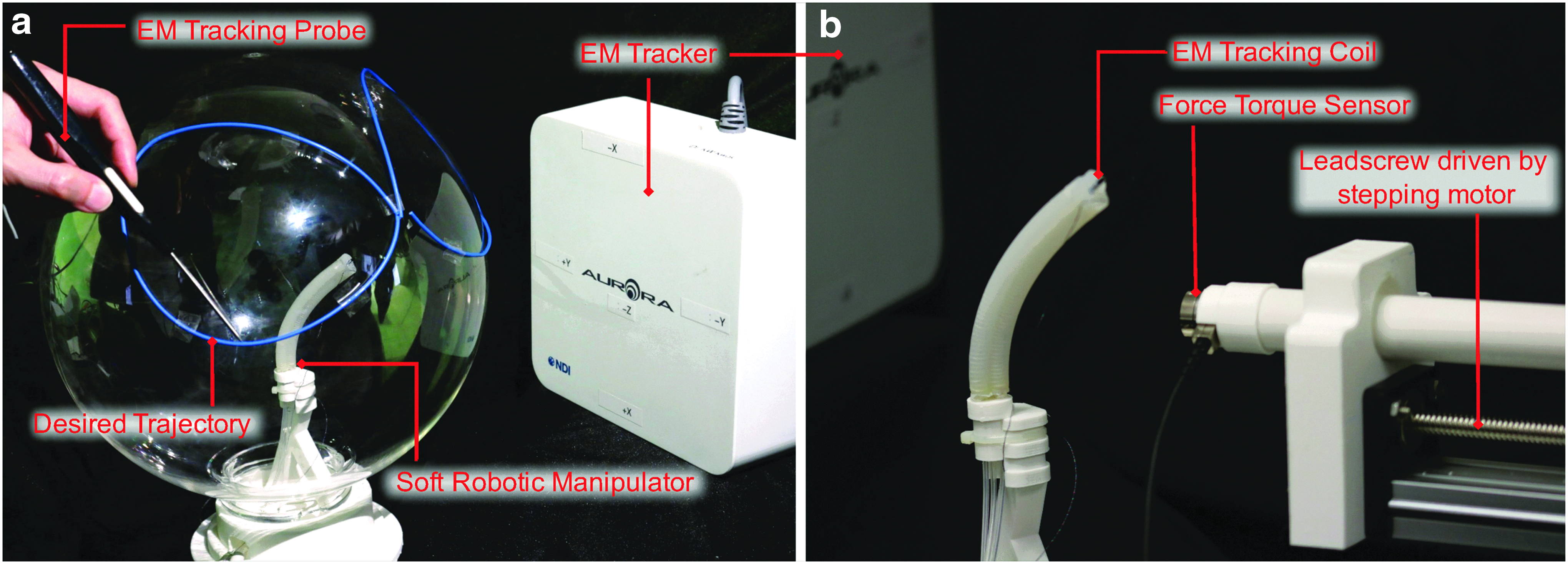
An EM tracking system (NDI Medical Aurora) is employed to close the robot control loop by the continuous positional data feedback (Fig. 7a). This tracking system is commonly available in many image-guided intervention systems. It can track the position and orientation of tiny EM coils in real time with root mean square (RMS) accuracy of 0.7 mm and 0.2° at 40 Hz. A tiny tracking coil is embedded at the robot distal tip. Online updating (at 20 Hz) of the inverse mapping estimation \documentclass{aastex}\usepackage{amsbsy}\usepackage{amsfonts}\usepackage{amssymb}\usepackage{bm}\usepackage{mathrsfs}\usepackage{pifont}\usepackage{stmaryrd}\usepackage{textcomp}\usepackage{portland, xspace}\usepackage{amsmath, amsxtra}\usepackage{upgreek}\pagestyle{empty}\DeclareMathSizes{10}{9}{7}{6}\begin{document} $$\Delta {{ \bf{u}}_k} = \Psi ( \Delta {{ \bf{s}}_k}^* , {{ \bf{s}}_k} , {{ \bf{u}}_k} )$$ \end{document} by the local learning algorithm is achieved, where \documentclass{aastex}\usepackage{amsbsy}\usepackage{amsfonts}\usepackage{amssymb}\usepackage{bm}\usepackage{mathrsfs}\usepackage{pifont}\usepackage{stmaryrd}\usepackage{textcomp}\usepackage{portland, xspace}\usepackage{amsmath, amsxtra}\usepackage{upgreek}\pagestyle{empty}\DeclareMathSizes{10}{9}{7}{6}\begin{document} $${{ \bf{s}}_k}$$ \end{document} is measured tip direction. The positional data are also recorded throughout the robot task so as to evaluate overall control performance. The entire control framework is implemented in the MATLAB environment. The open-source library of LWPR ⁵⁰ is employed to incrementally learn the robot forward model, which determines valid linearization of each local controller.

OPEN IN VIEWER

FIG. 7.

(a) Registration process of the predefined trajectory using an electromagnetic (EM) position tracking system. Blue line on the transparent sphere illustrates the tracking trajectory on the task space; (b) Soft manipulator is commanded to follow the desired trajectory automatically. Its end-effector position is also measured by the tracking system to close the feedback loop under online learning control policy. Plastic rod actuated by a stepping motor pushes against the soft robot, generating external constrains. The contact force is monitored by a force/torque sensor.

A series of path-following tasks is performed under various constraint scenarios to investigate how the online learning control approach reacts to such unknown interactions. At the beginning, the robot is allowed to move freely in its workspace without any interference. This serves as the control experiment to establish the baseline of controller performance. Subsequently, the robot is gently pushed by a plastic rod to simulate an unknown dynamic interaction with the robot manipulation (Fig. 7b). The rod is actuated by a high-precision stepping motor to generate repeatable contact with the robot body; meanwhile, the contact force is monitored by a force/torque sensor (ATI Industrial Automation: F/T Nano17). The tracking error is defined as the shortest distance between the robot targeting direction \documentclass{aastex}\usepackage{amsbsy}\usepackage{amsfonts}\usepackage{amssymb}\usepackage{bm}\usepackage{mathrsfs}\usepackage{pifont}\usepackage{stmaryrd}\usepackage{textcomp}\usepackage{portland, xspace}\usepackage{amsmath, amsxtra}\usepackage{upgreek}\pagestyle{empty}\DeclareMathSizes{10}{9}{7}{6}\begin{document} $${{ \bf{s}}_k}$$ \end{document} and the desired trajectory.

Evaluation of online local learning controller

To realize accurate navigation under unknown constraints, the inverse model is adapted in the proposed learning-based controller, which has to be updated online based on the newly acquired motion data. In this study, we compared three types of data sources for the inverse model training: (1) pretrained by FEA data without using online data; (2) initialized by random exploration with online learning data; and (3) pretrained by the FEA data, and then updated by online data. These online-updated inverse models are evaluated for resolved motion rate control ⁵¹ to track a predefined trajectory. Thus, the desired task space displacement \documentclass{aastex}\usepackage{amsbsy}\usepackage{amsfonts}\usepackage{amssymb}\usepackage{bm}\usepackage{mathrsfs}\usepackage{pifont}\usepackage{stmaryrd}\usepackage{textcomp}\usepackage{portland, xspace}\usepackage{amsmath, amsxtra}\usepackage{upgreek}\pagestyle{empty}\DeclareMathSizes{10}{9}{7}{6}\begin{document} $$\Delta { \bf{s}}_k^*$$ \end{document} that tracks the reference input is obtained as follows: \documentclass{aastex}\usepackage{amsbsy}\usepackage{amsfonts}\usepackage{amssymb}\usepackage{bm}\usepackage{mathrsfs}\usepackage{pifont}\usepackage{stmaryrd}\usepackage{textcomp}\usepackage{portland, xspace}\usepackage{amsmath, amsxtra}\usepackage{upgreek}\pagestyle{empty}\DeclareMathSizes{10}{9}{7}{6}\begin{document} \begin{align*} \Delta { \bf{s}}_k^* = \Delta { \bf{s}}_k^{ref} + { \bf{K}}_p^{ref} ( { \bf{s}}_k^{ref} - {{ \bf{s}}_k} ) \tag{13} \end{align*} \end{document}

where \documentclass{aastex}\usepackage{amsbsy}\usepackage{amsfonts}\usepackage{amssymb}\usepackage{bm}\usepackage{mathrsfs}\usepackage{pifont}\usepackage{stmaryrd}\usepackage{textcomp}\usepackage{portland, xspace}\usepackage{amsmath, amsxtra}\usepackage{upgreek}\pagestyle{empty}\DeclareMathSizes{10}{9}{7}{6}\begin{document} $$\Delta { \bf{s}}_k^{ref}$$ \end{document} and \documentclass{aastex}\usepackage{amsbsy}\usepackage{amsfonts}\usepackage{amssymb}\usepackage{bm}\usepackage{mathrsfs}\usepackage{pifont}\usepackage{stmaryrd}\usepackage{textcomp}\usepackage{portland, xspace}\usepackage{amsmath, amsxtra}\usepackage{upgreek}\pagestyle{empty}\DeclareMathSizes{10}{9}{7}{6}\begin{document} $${ \bf{s}}_k^{ref}$$ \end{document} are the reference task space displacements and coordinates generated from interpolating a predefined trajectory. Note that the reference input can be replaced by manual control in actual endoscopic navigation scenario. We employed the same proportional–derivative (PD) gain \documentclass{aastex}\usepackage{amsbsy}\usepackage{amsfonts}\usepackage{amssymb}\usepackage{bm}\usepackage{mathrsfs}\usepackage{pifont}\usepackage{stmaryrd}\usepackage{textcomp}\usepackage{portland, xspace}\usepackage{amsmath, amsxtra}\usepackage{upgreek}\pagestyle{empty}\DeclareMathSizes{10}{9}{7}{6}\begin{document} $${ \bf{K}}_p^{ref} = { \bf{I}}$$ \end{document} for all three settings to perform tracking along a reference trajectory. Thus, the actuation input \documentclass{aastex}\usepackage{amsbsy}\usepackage{amsfonts}\usepackage{amssymb}\usepackage{bm}\usepackage{mathrsfs}\usepackage{pifont}\usepackage{stmaryrd}\usepackage{textcomp}\usepackage{portland, xspace}\usepackage{amsmath, amsxtra}\usepackage{upgreek}\pagestyle{empty}\DeclareMathSizes{10}{9}{7}{6}\begin{document} $$\Delta {{ \bf{u}}_k}$$ \end{document} is estimated by the online learning inverse model as depicted in Equation (4).

To enforce the consistency of inverse mapping among all localized linear controllers, a standard null-space behavior \documentclass{aastex}\usepackage{amsbsy}\usepackage{amsfonts}\usepackage{amssymb}\usepackage{bm}\usepackage{mathrsfs}\usepackage{pifont}\usepackage{stmaryrd}\usepackage{textcomp}\usepackage{portland, xspace}\usepackage{amsmath, amsxtra}\usepackage{upgreek}\pagestyle{empty}\DeclareMathSizes{10}{9}{7}{6}\begin{document} $$\Delta {{ \bf{u}}_{0 , k}} = \upsilon ( {{ \bf{s}}_k} , {{ \bf{u}}_k} )$$ \end{document} is defined. This gives rise to an immediate reward function \documentclass{aastex}\usepackage{amsbsy}\usepackage{amsfonts}\usepackage{amssymb}\usepackage{bm}\usepackage{mathrsfs}\usepackage{pifont}\usepackage{stmaryrd}\usepackage{textcomp}\usepackage{portland, xspace}\usepackage{amsmath, amsxtra}\usepackage{upgreek}\pagestyle{empty}\DeclareMathSizes{10}{9}{7}{6}\begin{document} $$r ( \Delta {{ \bf{u}}_k} )$$ \end{document} to weigh the training data that best imitate the desired null-space behavior (Eq. 9). For the presented soft robot, we first choose a rest configuration to be \documentclass{aastex}\usepackage{amsbsy}\usepackage{amsfonts}\usepackage{amssymb}\usepackage{bm}\usepackage{mathrsfs}\usepackage{pifont}\usepackage{stmaryrd}\usepackage{textcomp}\usepackage{portland, xspace}\usepackage{amsmath, amsxtra}\usepackage{upgreek}\pagestyle{empty}\DeclareMathSizes{10}{9}{7}{6}\begin{document} $${{ \bf{u}}_{rest}} = { [ 0 , 0 , 0 ] ^{ \bf{T}}}$$ \end{document} , which can minimize the overall inflation pressure as well as elongation of the manipulator. Then, the robot is attracted toward the rest configuration with a loose attractor function \documentclass{aastex}\usepackage{amsbsy}\usepackage{amsfonts}\usepackage{amssymb}\usepackage{bm}\usepackage{mathrsfs}\usepackage{pifont}\usepackage{stmaryrd}\usepackage{textcomp}\usepackage{portland, xspace}\usepackage{amsmath, amsxtra}\usepackage{upgreek}\pagestyle{empty}\DeclareMathSizes{10}{9}{7}{6}\begin{document} $$\Delta {{ \bf{u}}_{0 , k}} = - {{ \bf{K}}_p} ( {{ \bf{u}}_k} - {{ \bf{u}}_{rest}} )$$ \end{document} , where \documentclass{aastex}\usepackage{amsbsy}\usepackage{amsfonts}\usepackage{amssymb}\usepackage{bm}\usepackage{mathrsfs}\usepackage{pifont}\usepackage{stmaryrd}\usepackage{textcomp}\usepackage{portland, xspace}\usepackage{amsmath, amsxtra}\usepackage{upgreek}\pagestyle{empty}\DeclareMathSizes{10}{9}{7}{6}\begin{document} $${{ \bf{K}}_p} = 0.2{ \bf{I}}$$ \end{document} . We defined an identity metric \documentclass{aastex}\usepackage{amsbsy}\usepackage{amsfonts}\usepackage{amssymb}\usepackage{bm}\usepackage{mathrsfs}\usepackage{pifont}\usepackage{stmaryrd}\usepackage{textcomp}\usepackage{portland, xspace}\usepackage{amsmath, amsxtra}\usepackage{upgreek}\pagestyle{empty}\DeclareMathSizes{10}{9}{7}{6}\begin{document} $${ \bf{N}} = { \bf{I}}$$ \end{document} as all three inflatable actuators of the robot are identical and should contribute the same in achieving the desired null-space behavior.

It is also necessary to normalize the training dataset into the same scale component-wise so that the LWPR can learn the data variance properly. Min-max normalization is a simple but effective technique commonly used ⁵² : \documentclass{aastex}\usepackage{amsbsy}\usepackage{amsfonts}\usepackage{amssymb}\usepackage{bm}\usepackage{mathrsfs}\usepackage{pifont}\usepackage{stmaryrd}\usepackage{textcomp}\usepackage{portland, xspace}\usepackage{amsmath, amsxtra}\usepackage{upgreek}\pagestyle{empty}\DeclareMathSizes{10}{9}{7}{6}\begin{document} \begin{align*} { \hat q_i } = { \frac { { q_i } - \min ( { q_i } ) } { \max ( { q_i } ) - \min ( { q_i } ) } } \tag { 14 } \end{align*} \end{document}

However, the statistical max(q_i) and min(q_i) values would be sensitive to outliers; therefore, we define the min–max values according to the physical constraints of data, including the typical robot workspace and the maximum volume of the cylinder unit.

Pretrained by FEA without using online data

In this setting, both the forward model and control policy are pretrained solely by the FEA-simulated data (see the Initialization of online learning by FEA-based model section). The online data were not taken into account in this setting. This acts as a control experiment to depict the actual influence of external interactions. In the unconstrained experiment (Fig. 8a), it was observed that the controller could roughly follow the trajectory with a relatively large tracking error of ±1.79° and a maximum error of ±6.96° with the use of the feedback controller (Table 1). Despite the considerable discrepancy between the FEA-simulated and actual configuration, this experiment still demonstrates that the FEA data are capable of pretraining a reasonable inverse model for rough path following.

OPEN IN VIEWER

FIG. 8.

Tracked trajectory plotted (left) and the corresponding tracking error in time domain (right). In the control experiment, the robot is allowed to move freely without any constraint. Control performance of the online learning controllers trained by three different data sources is validated: (a) Pretrained by FEA without using online data; (b) Pure online learning initialized by random exploration; (c) Pretrained by FEA data and updated by online data. The online learning initialized by the FEA data approach (c) combines the advantage of (a, b), in which random exploration (green path in (b)) is not required, but its tracking errors converge to similar accuracy as in pure online learning.

OPEN IN VIEWER

Table 1.

Trajectory Tracking Performance Under Freely Moveable Environment

	Mean absolute error		Maximum absolute error		Error SD \documentclass{aastex}\usepackage{amsbsy}\usepackage{amsfonts}\usepackage{amssymb}\usepackage{bm}\usepackage{mathrsfs}\usepackage{pifont}\usepackage{stmaryrd}\usepackage{textcomp}\usepackage{portland, xspace}\usepackage{amsmath, amsxtra}\usepackage{upgreek}\pagestyle{empty}\DeclareMathSizes{10}{9}{7}{6}\begin{document} $$\sigma$$ \end{document}
Training mode	First cycle	After	First cycle	After	First cycle	After
Pretrained by FEA only	±1.79°	±1.82°	±6.96°	±6.56°	1.71°	1.66°
Pure online learning	±1.13°	±0.87°	±4.24°	±1.92°	0.86°	0.45°
Combined	±2.21°	±0.90°	±7.49°	±2.80°	1.81°	0.65°

FEA, finite element analysis; SD, standard deviation.

In the later constrained experiment (Fig. 9a), the robot maintained tracking of the trajectory with similar accuracy at the beginning. When the external interaction is engaged at the moment of 25 s, the robot was pushed further away from the desired trajectory, resulting in an increased mean tracking error ±4.64° and a maximum error of ±14° (Table 2). This indicates that the feedback controller cannot fully compensate the significant motion bias that is induced by external disturbance.

OPEN IN VIEWER

FIG. 9.

Tracked trajectory plotted (left) and the corresponding tracking error in time domain (right) under external interactions. Control performance is validated in three different conditions as in Figure 8. It can be observed that online learning for (b, c) is capable of compensating the external interaction with the tracking error reduced, compared with the controller without using online data (a).

OPEN IN VIEWER

Table 2.

Trajectory Tracking Performance Under Constrained Environment

Training mode	Mean absolute error	Maximum absolute error	Error SD \documentclass{aastex}\usepackage{amsbsy}\usepackage{amsfonts}\usepackage{amssymb}\usepackage{bm}\usepackage{mathrsfs}\usepackage{pifont}\usepackage{stmaryrd}\usepackage{textcomp}\usepackage{portland, xspace}\usepackage{amsmath, amsxtra}\usepackage{upgreek}\pagestyle{empty}\DeclareMathSizes{10}{9}{7}{6}\begin{document} $$\sigma$$ \end{document}	Mean contact force	Maximum contact force
Pretrained by FEA only	±4.64°	±14.00°	3.20°	0.77N	1.06N
Pure online learning	±2.35°	±18.38°	2.47°	0.78N	0.97N
Combined	±2.49°	±11.03°	1.74°	0.80N	0.96N

In the case of a conventional rigid-linked robot, this kind of error due to the interaction with the constraint is often considered as a perturbation. The error can hence be compensated by increasing the feedback control gain given that the inverse model is readily available from the kinematic chain. However, such approach is not directly applicable to a soft robot due to their mechanical compliance that inevitably induces much larger positioning errors. In addition, the interaction force may also alter the force equilibrium of the robot and therefore substantially degrading the reliability of the predetermined inverse model. The following experiments demonstrate how the proposed online algorithm can accommodate the influence of constrained environment, which is particularly demanding for the control of soft robots.