Finite Element Method-Based Kinematics and Closed-Loop Control of Soft,Continuum Manipulators

Abstract

This article presents a modeling methodology and experimental validation for soft manipulators to obtain forward kinematic model (FKM) and inverse kinematic model (IKM) under quasi-static conditions (in the literature, these manipulators are usually classified as continuum robots. However, their main characteristic of interest in this article is that they create motion by deformation, as opposed to the classical use of articulations). It offers a way to obtain the kinematic characteristics of this type of soft robots that is suitable for offline path planning and position control. The modeling methodology presented relies on continuum mechanics, which does not provide analytic solutions in the general case. Our approach proposes a real-time numerical integration strategy based on finite element method with a numerical optimization based on Lagrange multipliers to obtain FKM and IKM. To reduce the dimension of the problem, at each step, a projection of the model to the constraint space (gathering actuators, sensors, and end-effector) is performed to obtain the smallest number possible of mathematical equations to be solved. This methodology is applied to obtain the kinematics of two different manipulators with complex structural geometry. An experimental comparison is also performed in one of the robots, between two other geometric approaches and the approach that is showcased in this article. A closed-loop controller based on a state estimator is proposed. The controller is experimentally validated and its robustness is evaluated using Lypunov stability method.

Introduction

For the past four decades, rigid-link manipulators have been successfully deployed in the industrial environment. Their rigid bodies and high torque joints are perfectly fitted to perform tasks that involve accurate positioning, while carrying considerable payloads. However, as the applications for these systems move away from this structured environment, traditional rigid manipulators have been less successful. Indeed, their rigid and bulky bodies are a problem for adaptation to dynamic environments.

Roboticists, trying to cope with the new applications for manipulators, have turned their attention to nature, seeking for inspiration to design new robot manipulators. Soft manipulators are robots often inspired by the morphology and functionality of biological agents like octopus tentacles and elephant trunks,^1–4 or tendrils.^5,6 This type of manipulator deforms continuously to achieve a certain pose and can exhibit key advantages over their rigid counterpart with suitable design: they are lighter and therefore have less energy consumption, and present a bigger power-to-weight ratio as well as a natural compliance because of their material properties. This compliance also gives the manipulators the ability to better adapt themselves to dynamic work environments and work side by side with humans, without the concern of hazardous collisions. Because of these characteristics, soft manipulators have found a niche of applications in the medical field.^7–11

The compliant nature of soft continuum manipulators comes with the issues of modeling and control of their behavior, which is highly nonlinear. A popular approach to model continuum robots has been the modification of methods already established to model rigid manipulators. In Ref.¹² Hannan and Walker presented the development of the kinematic model for a trunk robot. The model considers that each section bends with constant curvature. This approach has been used to express the kinematics of continuum trunks¹³ and tendril-like continuum robots.¹⁴ The constant curvature models can be used even when the shape of the continuum robot does not conform to a circular arc. In Ref.¹⁵ the kinematics of the bionic handling assistant are obtained by modeling each section of the robot as a finite number of serially connected circular arcs with different parameters each. The models mentioned, while producing close-form analytic models, are only based on the geometry of the robot, without consideration for the mechanics of the structure, necessary to properly describe the deformation of this type of robot.

Model requirements

In contrast with rigid robots, soft manipulator kinematics not only depend on the geometry of the robot but also on its mechanical properties, in particular the stiffness of the structure. While rigid manipulator kinematics can be used to solve positioning problems with the assumption of resistance/counter actuation to gravity or load effects, soft manipulators easily comply to these forces and deform. To answer the same problems of positioning, it is then necessary to take into account the current deformation (i.e., change of geometry) induced by these forces to obtain a kinematic relationship between position of end-effector and position of actuators (Fig. 1).

FIG. 1.

In this example, a tendon is pulled to create the motion of an elastic soft robot. Starting with the same geometry, the material stiffness has an influence on the kinematics (output vs. input displacements).

The degrees of freedom (DoFs) in a rigid manipulator are determined by the joints of the manipulator and are often all actuated. In soft manipulators, the DoFs are generated by the deformation of the continuum and their number is infinite. (It can be noted that it is disconnected from the number of actuators). Usually this problem is addressed by a discretization of the DoFs of the continuum, through methods provided by computational mechanics. Another difference in soft manipulators, compared with rigid ones, is that if a load is carried by a soft manipulator, this load will deform the robot and modify its kinematics.

Related work

This recapitulation of previous work is centralized in the use of continuum mechanics in the modeling of soft manipulators. A discussion on the use of mechanics-based methods to describe soft continuum robots can start by mentioning the work of Chirikjian and Burdick,^16,17 who used continuum mechanics to define a curve that describes the pose of hyper-redundant robots without considering actuation. This work laid the basis for subsequent work on continuum manipulator models.

Given the uprising trend in the design of manipulators composed by a single elongated backbone actuated by tendons, researchers have explored beam theory-based approaches to describe the pose of this particular type of robots. Rucker and Webster¹⁸ presented the potential of this theory applied to the modeling of manipulators with tendon routing. In Ref.¹⁹ the compliance model of continuum robots is obtained by considering the robot as a single section of Cosserat rod. In Ref.²⁰ Jones et al. present a static model in three-dimensional (3D) space, and in Ref.²¹ this theory was implemented to compute the inverse kinematic model (IKM) of a tendon-driven tentacle manipulator in two dimensions under Euler–Bernoulli beam hypothesis. While providing models suitable for fast computing, beam theory is limited in its application by the shape of the backbone, that is, when the backbone cannot be assimilated as a uniform beam, this modeling approach loses relevance. In particular, when the body of the robot is actuated intrinsically by pneumatic or hydraulic actuators, it tends to have a more complex shape, and its behavior cannot be described by beam theory methods. Finite element analysis is increasingly used in the field of soft robots. In Ref.²² a direct finite element simulation is used to observe the behavior of soft pneumatic actuators.

In this article, the development of a method to compute the kinematic model of soft manipulators that relies on the finite element model of the structure of the robot is presented. By using different types of elements (tetrahedral, beam, or shell elements), the methodology can be used on robots of very complex shapes. Contrary to the majority of models currently available in the literature, this approach also models two types of actuators, which enable this technique to be used as part of the control of the robot as well as in offline analysis. Moreover, gravity and payload carried by the end-effector can be accounted for by this approach.

This article presents the following contribution toward the kinematic modeling of soft manipulators:

A finite element method (FEM)-based modeling approach that accounts for complex structural shapes and the mechanics of the employed material.

The model of two actuation systems (i.e., pulling on cables and pneumatics) currently implemented in the majority of designs of soft manipulators.

The integration of sensors in the simulation that allow for an observer of the manipulator in the configuration space.

The validation of the modeling approach using two completely different deformable manipulators.

The experimental comparison of this approach to two other geometric-based models.

An experimental study on the robustness of the model under external loading.

A closed-loop controller based on a state estimator and the robustness analysis of the closed-loop system.

In the Methods section, the formulation of the static equilibrium and the constraints for end-effector, actuators, and sensors is explained. The Reduced Model in the Constraint Space section shows the projection of the model in the constraint space and the convex optimization process used to solve the reduced model. The Kinematic Models of a Soft Manipulator section presents the experimental validation of the FKM and IKM, and finally, in the FEM-Based Closed-Loop Control of Continuum Robots section, a discussion about the results and limitations of the model, as well as the perspectives for future work are presented.

Methods

In this section, the development of the FEM of soft manipulators is presented. The method relies on the constitutive law of the material from which the robot is made. This constitutive law can be directly measured by conducting stress/strain mechanical tests to a material sample in the ideal case. When the strain/stress tests cannot be done, an approximation of the constitutive law can be obtained in the simulation. The main idea is to tune these material parameters qualitatively by approximating the deformation seen in reality by that observed on simulation, in which the deformation of the real robot is matched given a known static load. A similar approach is presented in Ref.²³ in the context of radiotherapy. After measuring the constitutive law, a volume-based approach is used with tetrahedral elements. Then, the mathematical formulation of the constraints is introduced using Lagrange multipliers. In this method, the end-effector, actuators, and sensors use constraint models.

FEM model of soft and continuum robots

Depending on the shape of the robot, one could use volume, surface, or linear elements to compute the nonlinear deformation of the structure. In this article, volumetric elements^† are used. A nonlinear formulation accounts for the large displacements and rotations of the structure. In continuum mechanics, this is considered the case of large strain, but small stress. More sophisticated FEM models can be proposed in the future, according to the constitutive law and the solicitation of the employed material (i.e., large stress). The computation in real time with such models will be even more challenging, but the principles of the method described in this article would still apply.

The corotational implementation of volume FEM, presented in Ref.²⁴ is particularly suitable for linear elasticity under the hypothesis of large displacements. The shape of the robot is meshed using linear tetrahedral elements, but the same method could be used with other elements, shape functions, and more advanced material laws.

In the FEM, the nodes at the vertices of the elements represent the DoFs of the manipulator. Even for a considerable amount of nodes, the approach is fast to compute, numerically stable, and a free implementation in C++ is available in the open-source framework Simulation Open Framework Architecture (SOFA).²⁵ During each step i of the simulation, the following linearization of the internal forces is updated: \documentclass{aastex}\usepackage{amsbsy}\usepackage{amsfonts}\usepackage{amssymb}\usepackage{bm}\usepackage{mathrsfs}\usepackage{pifont}\usepackage{stmaryrd}\usepackage{textcomp}\usepackage{portland, xspace}\usepackage{amsmath, amsxtra}\usepackage{upgreek}\pagestyle{empty}\DeclareMathSizes{10}{9}{7}{6}\begin{document} \begin{align*} { \bf{f}} ( {{ \bf{x}}_i} ) \approx { \bf{f}} ( {{ \bf{x}}_{i - { \bf{1}}}} ) + { \bf{K}} ( {{ \bf{x}}_{{ \bf{i}} - { \bf{1}}}} ) d{ \bf{x}} , \tag{1} \end{align*} \end{document}

where f provides the volumetric internal stiffness forces at a given position x of the nodes, K(x) is the tangent stiffness matrix that depends on the actual positions of the nodes, and dx is the difference between positions dx = x_i − x_i−1. This linearization is valid as long as the displacement of the nodes dx is small. The lines and columns that correspond to fixed nodes are removed from the system to get a full rank for matrix K. In f and K, the rows (and columns for K) contain the component of the internal forces (x, y, z) for the nodes, in the order corresponding to their numbering in the mesh.

In this article, the study is limited to quasi-static behavior on purpose, since the simulation step required to capture high frequency vibrations is not feasible. Thus, in a first approach, the assumption is that the control of the robot is performed at low velocities, so that the inertia effects in the motion of the robot can be neglected.

One seeks to establish static equilibrium at each step from the first law of Newton: \documentclass{aastex}\usepackage{amsbsy}\usepackage{amsfonts}\usepackage{amssymb}\usepackage{bm}\usepackage{mathrsfs}\usepackage{pifont}\usepackage{stmaryrd}\usepackage{textcomp}\usepackage{portland, xspace}\usepackage{amsmath, amsxtra}\usepackage{upgreek}\pagestyle{empty}\DeclareMathSizes{10}{9}{7}{6}\begin{document} \begin{align*} {{ \bf{f}}_{{ \bf{ext}}}} + { \bf{f}} ( {{ \bf{x}}_{ \bf{i}}} ) + {{ \bf{H}}^T} \lambda = 0 , \tag{2} \end{align*} \end{document}

where f_ext represents the external forces (e.g., gravity) and H^T λ gathers the contributions of the end-effector, actuators, and the contact forces as Lagrange multipliers (see the following sections). The way H is obtained is explained in the Constraint for the end-effector, Actuator constraint model, and Sensor constraint model sections, but its computation is performed with the values obtained from the previous step. We then use the expression H(x_i₋₁) and through the linearization explained in Equation (1), we obtain the following formulation: \documentclass{aastex}\usepackage{amsbsy}\usepackage{amsfonts}\usepackage{amssymb}\usepackage{bm}\usepackage{mathrsfs}\usepackage{pifont}\usepackage{stmaryrd}\usepackage{textcomp}\usepackage{portland, xspace}\usepackage{amsmath, amsxtra}\usepackage{upgreek}\pagestyle{empty}\DeclareMathSizes{10}{9}{7}{6}\begin{document} \begin{align*} - { \bf{K}} ( {{ \bf{x}}_{{ \bf{i}} - { \bf{1}}}} ) d{ \bf{x}} = {{ \bf{f}}_{{ \bf{ext}}}} + { \bf{f}} ( {{ \bf{x}}_{{ \bf{i}} - { \bf{1}}}} ) + { \bf{H ( }}{{ \bf{x}}_{{ \bf{i}} - { \bf{1}}}}{{ \bf{ ) }}^T} \lambda \tag{3} \end{align*} \end{document}

The variables dx and λ are both unknown and are found during the optimization process.

It is noted that the matrix K is highly sparse. In the implementation, a conjugate gradient solver is used and preconditioned by a sparse LDL^T decomposition. For a mesh composed of about 1000 nodes and about 3000 tetrahedral elements, a refresh rate of 60 Hz is obtained with the implementation available in SOFA.

Constraint for the end-effector

To set the Lagrange multiplier on the end-effector, a point or a set of points of the robot needs to be considered the end-effector. It could be any point(s) mapped on the finite element (FE) mesh. For each point, the constraint objective is to reduce the difference between the end-effector position and its desired position p_des. Thus, a function δ _e(x): \documentclass{aastex}\usepackage{amsbsy}\usepackage{amsfonts}\usepackage{amssymb}\usepackage{bm}\usepackage{mathrsfs}\usepackage{pifont}\usepackage{stmaryrd}\usepackage{textcomp}\usepackage{portland, xspace}\usepackage{amsmath, amsxtra}\usepackage{upgreek}\pagestyle{empty}\DeclareMathSizes{10}{9}{7}{6}\begin{document} $${ \mathbb{R}^{3n}} \; \to \;{ \mathbb{R}^3}$$ \end{document} , with n being the number of nodes, evaluates this difference along x, y, and z. If the end-effector corresponds to a node i of the mesh, the function is δ _e(x) = x_i–p_des, where x_i is the position of node i. If the effector is set inside an element, we use \documentclass{aastex}\usepackage{amsbsy}\usepackage{amsfonts}\usepackage{amssymb}\usepackage{bm}\usepackage{mathrsfs}\usepackage{pifont}\usepackage{stmaryrd}\usepackage{textcomp}\usepackage{portland, xspace}\usepackage{amsmath, amsxtra}\usepackage{upgreek}\pagestyle{empty}\DeclareMathSizes{10}{9}{7}{6}\begin{document} \begin{align*} { \delta _e} ( { \bf{x}} ) = \sum \limits_{i = 0}^n { \phi _i} ( {{ \bf{p}}_{eff}} ) {{ \bf{x}}_i} , \tag{4} \end{align*} \end{document}

where p_eff is the position of the end-effector in the rest configuration of the FEM model and φ_i is the shape (interpolation) function associated to node i.

If several points are used for end-effector position, the vector δ_e(x) gathers the evaluation of the difference for all the points. The function is then \documentclass{aastex}\usepackage{amsbsy}\usepackage{amsfonts}\usepackage{amssymb}\usepackage{bm}\usepackage{mathrsfs}\usepackage{pifont}\usepackage{stmaryrd}\usepackage{textcomp}\usepackage{portland, xspace}\usepackage{amsmath, amsxtra}\usepackage{upgreek}\pagestyle{empty}\DeclareMathSizes{10}{9}{7}{6}\begin{document} $${ \mathbb{R}^{3n}} \; \to \;{ \mathbb{R}^{3m}}$$ \end{document} , where m is the number of end-effector points.

The matrix H used for the end-effectors corresponds to \documentclass{aastex}\usepackage{amsbsy}\usepackage{amsfonts}\usepackage{amssymb}\usepackage{bm}\usepackage{mathrsfs}\usepackage{pifont}\usepackage{stmaryrd}\usepackage{textcomp}\usepackage{portland, xspace}\usepackage{amsmath, amsxtra}\usepackage{upgreek}\pagestyle{empty}\DeclareMathSizes{10}{9}{7}{6}\begin{document} $$ { { \bf { H } } _e } ( { \bf { x } } ) = { \frac { \partial { \delta _e } ( { \bf { x } } ) } { \partial { \bf { x } } } } $$ \end{document} .

The matrix H_e is highly sparse: a row, which corresponds to a component of a point of the end-effector, will contain non-null values on a very small number of columns. As the point is mapped on a single tetrahedral element, there is a maximum of four non-null values per row. Of course, the column should match with the components of the nodes, given the fact that the non-null values are gathered in 3 × 3 diagonal block matrices.

Finally, an important point is the effort value that is put on the Lagrange multiplier that corresponds to the terminal effector. The value of λ_e will depend on the load applied on the end-effector. Two cases can be considered: (1) if the points defined as end-effector move freely in the space, there is no physical interaction, so the contribution of the constraint vanishes, λ_e = 0, and (2) if one or several points of the end-effector carry one object l which mass creates a load that could deform the structure. In such cases, the corresponding load should be set on λ_e = m_lg, with m_l the mass of the object and g the gravity field.

Actuator constraint model

In this work, the actuator model takes into account its physical characteristics. Two types of actuators have been implemented in the framework: tendon (cable) and pneumatic actuators. The contributions of these actuator constraints are unknown before the optimization process. However, given the type of actuation, the constraint is not set the same way.

Cable actuator

In a first case (Fig. 2), a cable is used to actuate the structure. The cable can simply be attached at one point of the structure, but it can also go through several other points (frictionless guides are considered). In all cases, the unknown λ_a is the stretching force inside the cable. This force is unilateral (λ_a ≥ 0).

FIG. 2.

Tendon actuation. d_b and d_a in the figure, represent the direction of the tendon before and after the cable guide, respectively, which are used to compute the normal forces at the guides.

Let us suppose now that the points are numbered starting from the extremity where the cable is being pulled. The matrix H is computed this way: at each point p, we take the direction of the cable before \documentclass{aastex}\usepackage{amsbsy}\usepackage{amsfonts}\usepackage{amssymb}\usepackage{bm}\usepackage{mathrsfs}\usepackage{pifont}\usepackage{stmaryrd}\usepackage{textcomp}\usepackage{portland, xspace}\usepackage{amsmath, amsxtra}\usepackage{upgreek}\pagestyle{empty}\DeclareMathSizes{10}{9}{7}{6}\begin{document} $$ { { \bf { d } } _b } = { \frac { { { \bf { x } } _p } - { { \bf { x } } _ { p - 1 } } } { \parallel { { \bf { x } } _p } - { { \bf { x } } _ { p - 1 } } \parallel } } $$ \end{document} and after \documentclass{aastex}\usepackage{amsbsy}\usepackage{amsfonts}\usepackage{amssymb}\usepackage{bm}\usepackage{mathrsfs}\usepackage{pifont}\usepackage{stmaryrd}\usepackage{textcomp}\usepackage{portland, xspace}\usepackage{amsmath, amsxtra}\usepackage{upgreek}\pagestyle{empty}\DeclareMathSizes{10}{9}{7}{6}\begin{document} $$ { { \bf { d } } _a } = { \frac { { { \bf { x } } _ { p + 1 } } - { { \bf { x } } _p } } { \parallel { { \bf { x } } _ { p + 1 } } - { { \bf { x } } _p } \parallel } } $$ \end{document} . To obtain the constraint direction that is applied to the point, we use d_p = d_a − d_b. Note that the direction of the final point is equal to the direction “before” as d_a does not exist. These constraint directions are mapped on the nodes using the following interpolation: \documentclass{aastex}\usepackage{amsbsy}\usepackage{amsfonts}\usepackage{amssymb}\usepackage{bm}\usepackage{mathrsfs}\usepackage{pifont}\usepackage{stmaryrd}\usepackage{textcomp}\usepackage{portland, xspace}\usepackage{amsmath, amsxtra}\usepackage{upgreek}\pagestyle{empty}\DeclareMathSizes{10}{9}{7}{6}\begin{document} \begin{align*} \left[ { \begin{matrix} \vdots \\ {{{ \bf{f}}_n}} \\ \vdots \\ \end{matrix} } \right] = \left[ { \begin{matrix} \vdots \\ {{ \phi _n} ( \alpha , \beta , \gamma ) \ {{ \bf{d}}_p}} \\ \vdots \\ \end{matrix} } \right] { \lambda _a} = { \bf{H}}_a^T{ \lambda _a} \tag{5} \end{align*} \end{document}

A function δ_a(x) is defined to provide the length of the cable, given the position of the constrained node(s). The actuator stroke can also be included by imposing \documentclass{aastex}\usepackage{amsbsy}\usepackage{amsfonts}\usepackage{amssymb}\usepackage{bm}\usepackage{mathrsfs}\usepackage{pifont}\usepackage{stmaryrd}\usepackage{textcomp}\usepackage{portland, xspace}\usepackage{amsmath, amsxtra}\usepackage{upgreek}\pagestyle{empty}\DeclareMathSizes{10}{9}{7}{6}\begin{document} $${ \delta _a} ( { \bf{x}} ) \in [ { \delta _{min}} \ { \delta _{max}} ]$$ \end{document} ). Through the use of this function, we get \documentclass{aastex}\usepackage{amsbsy}\usepackage{amsfonts}\usepackage{amssymb}\usepackage{bm}\usepackage{mathrsfs}\usepackage{pifont}\usepackage{stmaryrd}\usepackage{textcomp}\usepackage{portland, xspace}\usepackage{amsmath, amsxtra}\usepackage{upgreek}\pagestyle{empty}\DeclareMathSizes{10}{9}{7}{6}\begin{document} $$ { { \bf { H } } _a } = { \frac { \partial { \delta _a } ( { \bf { x } } ) } { \partial { \bf { x } } } } $$ \end{document} .

Pneumatic actuator

The formulation is compatible with pressure-based actuation of cavities that are placed on the structure (see Fig. 3). In that case, the effort λ_a is the pressure exerted on the wall of the cavity. As the pressure is uniform inside the cavity, a single constraint can be set for each pneumatic actuator. All triangles of the cavity wall will be involved: for each triangle t, the area and the normal direction are computed. If this result is multiplied by the pressure, one obtains the force applied by the pneumatic actuator on the nodes t of this triangle. Consequently, the contribution of each triangle is added in the corresponding column of \documentclass{aastex}\usepackage{amsbsy}\usepackage{amsfonts}\usepackage{amssymb}\usepackage{bm}\usepackage{mathrsfs}\usepackage{pifont}\usepackage{stmaryrd}\usepackage{textcomp}\usepackage{portland, xspace}\usepackage{amsmath, amsxtra}\usepackage{upgreek}\pagestyle{empty}\DeclareMathSizes{10}{9}{7}{6}\begin{document} $${ \bf{H}}_a^T$$ \end{document} .

FIG. 3.

Pressure actuation.

In the particular case of a pneumatic actuation, λ_a provides the difference of pressure inside the cavity compared with the atmospheric pressure. Usually, pneumatic actuators only provide positive pressure, so λ_a ≥ 0. However, in some cases, it is also possible to create both negative and positive pressure using vacuum/pressure actuation. In that case, there is no particular constraint on the unknown value of λ_a, despite an eventual limit (max/min) of pressure that can be achieved by the actuator.

The approach to the modeling of fluidic actuators can also account for hydraulic actuators, by accounting for the weight distribution of the liquid at any given configuration, as presented in Ref.²⁶

Sensor constraint model

To relate the end-effector position and the geometry of the manipulator, one needs sensors that can measure the geometric state of the robot. In this study, the sensors used can measure the lengths of the sections that compose the manipulator, but also that can be easily integrated in the design. String potentiometers offer a good solution to acquire information on the real geometric state of the robot. As in the case of the cable actuator, the string of the sensor is routed through several frictionless guides, at n points, x_n. In the model, the measure of the lengths read by the sensor will be as follows: \documentclass{aastex}\usepackage{amsbsy}\usepackage{amsfonts}\usepackage{amssymb}\usepackage{bm}\usepackage{mathrsfs}\usepackage{pifont}\usepackage{stmaryrd}\usepackage{textcomp}\usepackage{portland, xspace}\usepackage{amsmath, amsxtra}\usepackage{upgreek}\pagestyle{empty}\DeclareMathSizes{10}{9}{7}{6}\begin{document} \begin{align*} \sum \limits_{i = 1}^{n - 1} \parallel {{ \bf{x}}_{i + 1}} - {{ \bf{x}}_i} \parallel , \tag{6} \end{align*} \end{document}

which evaluates the distance between each sensor guide after the position of the nodes have been updated. A function δ_s is defined to represent the difference between the current lengths of the sensors and the desired lengths. The matrix H_s that gathers the directions of the sensor constraint is obtained in the same way as for the cable actuator, shown in the Cable actuator section.

Reduced Model in the Constraint Space

The classical resolution of a FEM problem (like solving the static equilibrium of the structure described at Eq. 3) provides a forward model: it allows to compute the displacements of the structure, given the values of the efforts put on the actuator λ_a. However, in the case of position control, the actuation λ_a is the unknown. Yet, for controlling the motion of the soft robot, an inverse model is needed, which is challenging to compute in real time as the size of the system is in the range of several thousand DoFs. In this work, another approach is used, based on the projection of the mechanics in the constraint space that drastically reduces the size of the optimization problem. This approach, initially developed in Ref.²⁷ is generalized. A new formulation of the inverse problem in the form of a quadratic programming (QP) optimization (developed in Ref.²⁸) is used.

Reduced compliance in constraint space

As stated previously, the optimization process relies on a projection of the mechanics in the constraint space. Each constraint has a direction that is set by a line of the matrices H_e and H_a

This matrix is sparse, as the direction of the constraints is mapped on few nodes of the FE mesh. The values of the effort applied by the actuators λ_a are not known at the beginning of the optimization process, whereas the value of λ_e is supposed to be known.

The first step consists of obtaining a free configuration x_free of the robot, which is found by solving the Equation (3), while considering that there is no actuation applied to the deformable structure. In practice, the known value of λ_e is used and λ_a = 0 is imposed.

The linear Equation (3) is solved using a LDL^T factorization of the matrix K. Given this new free position x_free for all the nodes of the mesh, one can evaluate the values of \documentclass{aastex}\usepackage{amsbsy}\usepackage{amsfonts}\usepackage{amssymb}\usepackage{bm}\usepackage{mathrsfs}\usepackage{pifont}\usepackage{stmaryrd}\usepackage{textcomp}\usepackage{portland, xspace}\usepackage{amsmath, amsxtra}\usepackage{upgreek}\pagestyle{empty}\DeclareMathSizes{10}{9}{7}{6}\begin{document} $$\delta _e^{{ \rm{free}}} = { \delta _e} ( {{ \bf{x}}_{{ \rm{free}}}} )$$ \end{document} , the shift between the effector point(s) position and the desired position introduced in the Constraint for the End-Effector section. One can also evaluate \documentclass{aastex}\usepackage{amsbsy}\usepackage{amsfonts}\usepackage{amssymb}\usepackage{bm}\usepackage{mathrsfs}\usepackage{pifont}\usepackage{stmaryrd}\usepackage{textcomp}\usepackage{portland, xspace}\usepackage{amsmath, amsxtra}\usepackage{upgreek}\pagestyle{empty}\DeclareMathSizes{10}{9}{7}{6}\begin{document} $$\delta _a^{{ \rm{free}}} = { \delta _a} ( {{ \bf{x}}_{{ \rm{free}}}} )$$ \end{document} , the position of the actuated points without actuation effort.

From the FEM formulation of the problem that uses a large matrix K, a formulation that accounts for the directions of the constraints placed for actuators and end-effectors is derived. Using the Schur complement of matrix K in the Lagrange multiplier-augmented system,²⁹ a small formulation of δ_e is obtained. This variable expresses the difference between the desired position for the end-effector and its current position in terms of the actuator contributions λ_a: \documentclass{aastex}\usepackage{amsbsy}\usepackage{amsfonts}\usepackage{amssymb}\usepackage{bm}\usepackage{mathrsfs}\usepackage{pifont}\usepackage{stmaryrd}\usepackage{textcomp}\usepackage{portland, xspace}\usepackage{amsmath, amsxtra}\usepackage{upgreek}\pagestyle{empty}\DeclareMathSizes{10}{9}{7}{6}\begin{document} \begin{align*} { \delta _e} = \underbrace { \left[ {{{ \bf{H}}_e}{{ \bf{K}}^{ - 1}}{ \bf{H}}_a^T} \right] }_{{{ \bf{W}}_{ea}}}{ \lambda _a} + \delta _e^{{ \rm{free}}} \tag{7} \end{align*} \end{document}

The Schur complement also provides similar formulations for the difference between a desired sensor or actuator position and its current position: \documentclass{aastex}\usepackage{amsbsy}\usepackage{amsfonts}\usepackage{amssymb}\usepackage{bm}\usepackage{mathrsfs}\usepackage{pifont}\usepackage{stmaryrd}\usepackage{textcomp}\usepackage{portland, xspace}\usepackage{amsmath, amsxtra}\usepackage{upgreek}\pagestyle{empty}\DeclareMathSizes{10}{9}{7}{6}\begin{document} \begin{align*} { \delta _a} = \underbrace { \left[ {{{ \bf{H}}_a}{{ \bf{K}}^{ - 1}}{ \bf{H}}_a^T} \right] }_{{{ \bf{W}}_{aa}}}{ \lambda _a} + \delta _a^{{ \rm{free}}} \tag{8} \end{align*} \end{document} \documentclass{aastex}\usepackage{amsbsy}\usepackage{amsfonts}\usepackage{amssymb}\usepackage{bm}\usepackage{mathrsfs}\usepackage{pifont}\usepackage{stmaryrd}\usepackage{textcomp}\usepackage{portland, xspace}\usepackage{amsmath, amsxtra}\usepackage{upgreek}\pagestyle{empty}\DeclareMathSizes{10}{9}{7}{6}\begin{document} \begin{align*} { \delta _s} = \underbrace { \left[ {{{ \bf{H}}_s}{{ \bf{K}}^{ - 1}}{ \bf{H}}_a^T} \right] }_{{{ \bf{W}}_{sa}}}{ \lambda _a} + \delta _s^{{ \rm{free}}} \tag{9} \end{align*} \end{document}

This step is central in the method. It consists in projecting the mechanics into the constraint space. As the constraints are the inputs (effector position shift and sensor length shift) and outputs (effort to apply on the actuators) of the inverse problem, the smallest possible projection space for the inverse problem is obtained. It allows for a projection that drastically reduces the size of the search space without loss of information. Indeed, the section Coupled kinematic equations shows how the matrices W_ea and W_aa provide the mechanical coupling equations between actuators and effector point(s).

After this projection, the optimization is processed in the reduced constraint space to get the values of λ_a. This part is described in the Inverse Model by Convex Optimization section.

The final configuration of the soft robot, at the end of the time step, is obtained as follows: \documentclass{aastex}\usepackage{amsbsy}\usepackage{amsfonts}\usepackage{amssymb}\usepackage{bm}\usepackage{mathrsfs}\usepackage{pifont}\usepackage{stmaryrd}\usepackage{textcomp}\usepackage{portland, xspace}\usepackage{amsmath, amsxtra}\usepackage{upgreek}\pagestyle{empty}\DeclareMathSizes{10}{9}{7}{6}\begin{document} \begin{align*} {{ \bf{x}}_t} = {{ \bf{x}}_{{ \rm{free}}}} + {{ \bf{K}}^{ - 1}}{ \bf{H}}_a^T{ \lambda _a}. \tag{10} \end{align*} \end{document}

It should be emphasized that one of the main difficulties is to compute W_ea and W_aa in a fast manner. No precomputation is possible as their value changes at each iteration. However, this type of projection problem is frequent when solving friction contact on deformable objects. Thus, several strategies are already implemented in SOFA.²⁵

Coupled kinematic equations

Using the compliance operator W_ea, one can get a measure of the mechanical coupling between effector and actuator, and with W_aa, the coupling between actuators.

For instance, the displacement \documentclass{aastex}\usepackage{amsbsy}\usepackage{amsfonts}\usepackage{amssymb}\usepackage{bm}\usepackage{mathrsfs}\usepackage{pifont}\usepackage{stmaryrd}\usepackage{textcomp}\usepackage{portland, xspace}\usepackage{amsmath, amsxtra}\usepackage{upgreek}\pagestyle{empty}\DeclareMathSizes{10}{9}{7}{6}\begin{document} $$\delta _e^i$$ \end{document} created on the end-effector (along a direction stored on the line i of matrix H_e) by a unitary force \documentclass{aastex}\usepackage{amsbsy}\usepackage{amsfonts}\usepackage{amssymb}\usepackage{bm}\usepackage{mathrsfs}\usepackage{pifont}\usepackage{stmaryrd}\usepackage{textcomp}\usepackage{portland, xspace}\usepackage{amsmath, amsxtra}\usepackage{upgreek}\pagestyle{empty}\DeclareMathSizes{10}{9}{7}{6}\begin{document} $$\lambda _a^j$$ \end{document} applied by the actuator (which is stored at the line j of matrix H_a) is directly obtained by \documentclass{aastex}\usepackage{amsbsy}\usepackage{amsfonts}\usepackage{amssymb}\usepackage{bm}\usepackage{mathrsfs}\usepackage{pifont}\usepackage{stmaryrd}\usepackage{textcomp}\usepackage{portland, xspace}\usepackage{amsmath, amsxtra}\usepackage{upgreek}\pagestyle{empty}\DeclareMathSizes{10}{9}{7}{6}\begin{document} $$\Delta \delta _e^i = w_{ea}^{ij} \lambda _a^j + \delta _e^{i , { \rm{free}}}$$ \end{document} .

As the motion is created by deformation, the motion of actuator j is influenced by actuator k.

Through the same principle, actuator k also influences the displacement of the effector. To get a kinematic link between actuators and effector, the method needs to account for the mechanical coupling that can exist between actuators. It is captured by W_aa that can be inverted if actuators are defined on independent DoFs. Thus, one can get a kinematic link by rewriting Equation (8) as follows: \documentclass{aastex}\usepackage{amsbsy}\usepackage{amsfonts}\usepackage{amssymb}\usepackage{bm}\usepackage{mathrsfs}\usepackage{pifont}\usepackage{stmaryrd}\usepackage{textcomp}\usepackage{portland, xspace}\usepackage{amsmath, amsxtra}\usepackage{upgreek}\pagestyle{empty}\DeclareMathSizes{10}{9}{7}{6}\begin{document} \begin{align*} { \delta _e} = {{ \bf{W}}_{ea}}{ \bf{W}}_{aa}^{ - 1} ( { \delta _a} - \delta _a^{{ \rm{free}}} ) + \delta _e^{{ \rm{free}}} \tag{11} \end{align*} \end{document}

Equation (11) is composed of a reduced number of linear equations that relate the displacement of the actuators to the displacement of the effector. Consequently, matrix \documentclass{aastex}\usepackage{amsbsy}\usepackage{amsfonts}\usepackage{amssymb}\usepackage{bm}\usepackage{mathrsfs}\usepackage{pifont}\usepackage{stmaryrd}\usepackage{textcomp}\usepackage{portland, xspace}\usepackage{amsmath, amsxtra}\usepackage{upgreek}\pagestyle{empty}\DeclareMathSizes{10}{9}{7}{6}\begin{document} $${{ \bf{W}}_{ea}}{ \bf{W}}_{aa}^{ - 1}$$ \end{document} is equivalent to the Jacobian matrix of a rigid manipulator. This matrix is a local linearization provided by the FEM model on a given position. It needs to be updated for deformations with large displacements.

Inverse model by convex optimization

The goal of the optimization is to find how to actuate the structure so that the end-effector of the robot reaches a desired position. This was initially proposed in Ref.²⁸ It consists in reducing the norm of δ_e, which actually measures the shift between the end-effector and its desired position. Thus, computing \documentclass{aastex}\usepackage{amsbsy}\usepackage{amsfonts}\usepackage{amssymb}\usepackage{bm}\usepackage{mathrsfs}\usepackage{pifont}\usepackage{stmaryrd}\usepackage{textcomp}\usepackage{portland, xspace}\usepackage{amsmath, amsxtra}\usepackage{upgreek}\pagestyle{empty}\DeclareMathSizes{10}{9}{7}{6}\begin{document} $$min ( \frac { 1 } { 2 } \delta _e^T { \delta _e } )$$ \end{document} leads to a QP problem: \documentclass{aastex}\usepackage{amsbsy}\usepackage{amsfonts}\usepackage{amssymb}\usepackage{bm}\usepackage{mathrsfs}\usepackage{pifont}\usepackage{stmaryrd}\usepackage{textcomp}\usepackage{portland, xspace}\usepackage{amsmath, amsxtra}\usepackage{upgreek}\pagestyle{empty}\DeclareMathSizes{10}{9}{7}{6}\begin{document} \begin{align*} min \left ( {{1 \over 2}{ \lambda _a}^T{ \bf{W}}_{ea}^T{{ \bf{W}}_{ea}}{ \lambda _a} + { \lambda _a}^T{ \bf{W}}_{ea}^T \delta _e^{{ \rm{free}}}} \right ) \tag { 12 } \end{align*} \end{document} \documentclass{aastex}\usepackage{amsbsy}\usepackage{amsfonts}\usepackage{amssymb}\usepackage{bm}\usepackage{mathrsfs}\usepackage{pifont}\usepackage{stmaryrd}\usepackage{textcomp}\usepackage{portland, xspace}\usepackage{amsmath, amsxtra}\usepackage{upgreek}\pagestyle{empty}\DeclareMathSizes{10}{9}{7}{6}\begin{document} \begin{align*} \begin{matrix} {subject \ to \ { \rm{ ( course}} \ { \rm{of}} \ { \rm{actuators ) :}}} \hfill \\ {{ \delta _{min}} \le { \delta _a} = {{ \bf{W}}_{aa}}{ \lambda _a} + \delta _a^{{ \rm{free}}} \le { \delta _{max}}} \hfill \\ {and \ { \rm{ ( case}} \ { \rm{of}} \ { \rm{unilateral}} \ { \rm{effort}} \ { \rm{actuation ) :}}} \hfill \\ {{ \lambda _a} \ge 0} \hfill \\ \end{matrix} \tag{13} \end{align*} \end{document}

The use of a minimization allows to find a solution even when the desired position is out of the workspace of the robot. In such a case, the algorithm will find the point that minimizes the distance to the desired position, while staying in the limits introduced by the course of the actuators.

In practice, the QP solver available in the Computational Geometry Algorithms Library³⁰ is used. The matrix of the QP \documentclass{aastex}\usepackage{amsbsy}\usepackage{amsfonts}\usepackage{amssymb}\usepackage{bm}\usepackage{mathrsfs}\usepackage{pifont}\usepackage{stmaryrd}\usepackage{textcomp}\usepackage{portland, xspace}\usepackage{amsmath, amsxtra}\usepackage{upgreek}\pagestyle{empty}\DeclareMathSizes{10}{9}{7}{6}\begin{document} $${ \bf{W}}_{ea}^T{{ \bf{W}}_{ea}}$$ \end{document} is symmetric. If the number of actuators is equal or inferior to the size of the end-effector space, the matrix is also definite. In such a case, the solution of the minimization is unique.

In the case when the number of actuators is greater than the DoFs of the effector points, the matrix of the QP is only semidefinite. Consequently, the solution could be nonunique.

A new criterion for the minimization can be introduced, based on the deformation energy. Indeed, this energy E_def is linked to the mechanical work of the forces exerted by the actuators. E_def can be computed by evaluating the dot product between λ_a and the displacements of the actuators \documentclass{aastex}\usepackage{amsbsy}\usepackage{amsfonts}\usepackage{amssymb}\usepackage{bm}\usepackage{mathrsfs}\usepackage{pifont}\usepackage{stmaryrd}\usepackage{textcomp}\usepackage{portland, xspace}\usepackage{amsmath, amsxtra}\usepackage{upgreek}\pagestyle{empty}\DeclareMathSizes{10}{9}{7}{6}\begin{document} $$\Delta { \delta _a} = { \delta _a} - \delta _a^{{ \rm{free}}}$$ \end{document} due to the actuator forces \documentclass{aastex}\usepackage{amsbsy}\usepackage{amsfonts}\usepackage{amssymb}\usepackage{bm}\usepackage{mathrsfs}\usepackage{pifont}\usepackage{stmaryrd}\usepackage{textcomp}\usepackage{portland, xspace}\usepackage{amsmath, amsxtra}\usepackage{upgreek}\pagestyle{empty}\DeclareMathSizes{10}{9}{7}{6}\begin{document} $${E_{def}} = { \lambda _a}^T \Delta { \delta _a} = { \lambda _a}^T{{ \bf{W}}_{aa}}{ \lambda _a}$$ \end{document} . Yet, matrix W_aa is positive definite if the actuators are placed on different nodes of the FEM or with different directions (i.e., if there is no linear dependencies between lines of H_a). Thus, one can add this energy in the minimization process by replacing Equation (12) with \documentclass{aastex}\usepackage{amsbsy}\usepackage{amsfonts}\usepackage{amssymb}\usepackage{bm}\usepackage{mathrsfs}\usepackage{pifont}\usepackage{stmaryrd}\usepackage{textcomp}\usepackage{portland, xspace}\usepackage{amsmath, amsxtra}\usepackage{upgreek}\pagestyle{empty}\DeclareMathSizes{10}{9}{7}{6}\begin{document} \begin{align*} min \left( { \frac { 1 } { 2 } { \lambda _a } ^T ( { \bf { W } } _ { ea } ^T { { \bf { W } } _ { ea } } + \varepsilon { { \bf { W } } _ { aa } } ) { \lambda _a } + { \lambda _a } ^T { \bf { W } } _ { ea } ^T \delta _e^ { { \rm { free } } } } \right) , \tag { 14 } \end{align*} \end{document}

where ɛ chosen sufficiently small so that the deformation energy does not disrupt the quality of the effector positioning. In practice, \documentclass{aastex}\usepackage{amsbsy}\usepackage{amsfonts}\usepackage{amssymb}\usepackage{bm}\usepackage{mathrsfs}\usepackage{pifont}\usepackage{stmaryrd}\usepackage{textcomp}\usepackage{portland, xspace}\usepackage{amsmath, amsxtra}\usepackage{upgreek}\pagestyle{empty}\DeclareMathSizes{10}{9}{7}{6}\begin{document} $$\varepsilon = { \frac { tr ( { \bf { W } } _ { ea } ^T { { \bf { W } } _ { ea } } ) } { tr ( { { \bf { W } } _ { aa } } ) } } { *10^ { - 3 } } $$ \end{document} , so that the term ɛW_aa does not alter the value of the QP matrix. Thanks to this modification, the QP matrix becomes positive definite and a unique solution of the problem can be found.

Kinematic Models of a Soft Manipulator

In this section, the proposed methodology is validated experimentally by obtaining FKM and IKM of the compact bionic handling assistant (CBHA). The forward model is compared with two geometric models developed for the same robot. The simulation in real time of the IKM is used in open loop to control the position of the end-effector of the manipulator. A proof of genericness is given by modeling a second soft manipulator inspired by parallel robots actuated by tendons with clear geometric differences and material characteristics.

Description of the CBHA

The CBHA is the bionic continuum manipulator component of the RobotinoXT, a didactic mobile platform designed by Festo Robotics. The system is shown in Figure 4 (left). The bionic continuum manipulator is formed by two serially connected sections of pneumatic actuators, an axially rotating wrist and a compliant gripper. Without actuation, the manipulator has a length of 206 mm, with each section having a length of 103 mm. The width at the base of the manipulator is 100 mm long and the top has 80 mm of width. In our study, the end of the second section is considered the end-effector.

FIG. 4.

The RobotinoXT by Festo Robotics. Left: The anatomy of the CBHA. Right: A section of the manipulator, composed by three pneumatic actuators and their correspondent length sensor. CBHA, compact bionic handling assistant.

Each section of the manipulator is composed of a parallel array of pneumatic actuators, as shown in Figure 4 (right). By applying different pressures to the bellows, each section can bend or extend independently. The pose of the manipulator is obtained as the contribution of the poses of the two sections. To sense the state of the robot, string potentiometers measure the lengths of the actuators.

Forward kinematic model

The FKM of a soft manipulator deals with the problem of finding the end-effector position, given a defined configuration of the manipulator. For a rigid manipulator, this configuration is simply the set of variables associated with the joints of the robot. In contrast with the rigid robots, the variables that express the configuration of a soft manipulator change with respect to the structure of the robot and its type of actuation, and therefore cannot be obtained in a straight-forward manner. The FEM-based methods explained before provide an easy way to obtain the kinematic relationship between the end-effector and the configuration of the manipulator.

FEM-based model

Given the intrinsic nature of the CBHA, the configuration of the robot is represented by the lengths of the pneumatic actuators that correspond to an end-effector position. Of course, the description of the robot could be given in the actuator space directly, using in this case Equation (7), to attain a pressure-to-position model, but that requires a precise control over the actuation (in this case, the pressure inside the cavities) to obtain a good estimation of the position of the end-effector. Instead, Equation (9), which is reproduced here for clarification, is used to relate the end-effector position to the configuration of the manipulator represented by the lengths of each pneumatic actuator, given by the sensors. This representation is clearer in the context of kinematic modeling, and allows for a position-to-position model, which is less sensitive to unknown hardware parameters: \documentclass{aastex}\usepackage{amsbsy}\usepackage{amsfonts}\usepackage{amssymb}\usepackage{bm}\usepackage{mathrsfs}\usepackage{pifont}\usepackage{stmaryrd}\usepackage{textcomp}\usepackage{portland, xspace}\usepackage{amsmath, amsxtra}\usepackage{upgreek}\pagestyle{empty}\DeclareMathSizes{10}{9}{7}{6}\begin{document} \begin{align*} { \delta _s} = \underbrace { \left[ {{{ \bf{H}}_s}{{ \bf{K}}^{ - 1}}{ \bf{H}}_a^T} \right] }_{{{ \bf{W}}_{sa}}}{ \lambda _a} + \delta _s^{{ \rm{free}}} \tag{15} \end{align*} \end{document}

In this approach, no geometrical assumptions are needed. Each part of the robot is modeled in detail using shell and tetrahedral elements, as presented in Figure 5. The mesh used in the model of the pneumatic cavities is composed by 3528 elements.

FIG. 5.

Visual model of the trunk and the underlying finite element model.

Once the constraints have been incorporated in the model, the convex optimization finds each actuator contribution required to have the desired sensor lengths. The final position of the end-effector is obtained after the position of the nodes of the mesh is updated.

Constant curvature model

This model of the CBHA, which was developed in Refs.^31,32 and validated in Ref.³¹ works under the assumption that, after actuation, the resulting pose of each section in the robot can be represented by an arc section with constant curvature (Fig. 6).

FIG. 6.

Constant curvature model.

The evolution from end to end of a section i is described, in terms of backbone parameters, by two coupled rotations and one translation in the homogeneous transformations: \documentclass{aastex}\usepackage{amsbsy}\usepackage{amsfonts}\usepackage{amssymb}\usepackage{bm}\usepackage{mathrsfs}\usepackage{pifont}\usepackage{stmaryrd}\usepackage{textcomp}\usepackage{portland, xspace}\usepackage{amsmath, amsxtra}\usepackage{upgreek}\pagestyle{empty}\DeclareMathSizes{10}{9}{7}{6}\begin{document} \begin{align*} _{ \rm{j}}^{ \rm{i}}{ \rm{T}} = \left[ { \begin{matrix} {{c^2}{ \phi _i}c{ \theta _i} + {s^2}{ \phi _i}} & {c{ \phi _i}s{ \phi _i} ( c{ \theta _i} - 1 ) } & {c{ \phi _i}s{ \theta _i}} & {{x_i}} \\ {c{ \phi _i}s{ \phi _i} ( c{ \theta _i} - 1 ) } & {{s^2}{ \phi _i}c{ \theta _i} + {c^2}{ \phi _i}} & {s{ \phi _i}s{ \theta _i}} & {{y_i}} \\ { - c{ \phi _i}s{ \theta _i}} & { - s{ \phi _i}s{ \theta _i}} & {c{ \theta _i}} & {{z_i}} \\ 0 & 0 & 0 & 1 \\ \end{matrix} } \right] , \tag{16} \end{align*} \end{document}

where the notations s and c mean sine and cosine, respectively. The Cartesian coordinates of the end of the bending section i are given by (x_i, y_i, and z_i), where \documentclass{aastex}\usepackage{amsbsy}\usepackage{amsfonts}\usepackage{amssymb}\usepackage{bm}\usepackage{mathrsfs}\usepackage{pifont}\usepackage{stmaryrd}\usepackage{textcomp}\usepackage{portland, xspace}\usepackage{amsmath, amsxtra}\usepackage{upgreek}\pagestyle{empty}\DeclareMathSizes{10}{9}{7}{6}\begin{document} $${x_i} = {r_i}c{ \phi _i} ( 1 - c{ \theta _i} )$$ \end{document} , \documentclass{aastex}\usepackage{amsbsy}\usepackage{amsfonts}\usepackage{amssymb}\usepackage{bm}\usepackage{mathrsfs}\usepackage{pifont}\usepackage{stmaryrd}\usepackage{textcomp}\usepackage{portland, xspace}\usepackage{amsmath, amsxtra}\usepackage{upgreek}\pagestyle{empty}\DeclareMathSizes{10}{9}{7}{6}\begin{document} $${y_i} = {r_i}s{ \phi _i} ( 1 - c{ \theta _i} )$$ \end{document} , and \documentclass{aastex}\usepackage{amsbsy}\usepackage{amsfonts}\usepackage{amssymb}\usepackage{bm}\usepackage{mathrsfs}\usepackage{pifont}\usepackage{stmaryrd}\usepackage{textcomp}\usepackage{portland, xspace}\usepackage{amsmath, amsxtra}\usepackage{upgreek}\pagestyle{empty}\DeclareMathSizes{10}{9}{7}{6}\begin{document} $${z_i} = {r_i}s{ \theta _i}$$ \end{document} . The backbone variables φ_i, θ_i, and r_i can be expressed in terms of the actuator lengths to have the correct kinematic relationships: \documentclass{aastex}\usepackage{amsbsy}\usepackage{amsfonts}\usepackage{amssymb}\usepackage{bm}\usepackage{mathrsfs}\usepackage{pifont}\usepackage{stmaryrd}\usepackage{textcomp}\usepackage{portland, xspace}\usepackage{amsmath, amsxtra}\usepackage{upgreek}\pagestyle{empty}\DeclareMathSizes{10}{9}{7}{6}\begin{document} \begin{align*} {{\phi_i}} & = {tan^{-1}} \left( \frac{{\sqrt 3 ({l_3} - {l_1})}} {{2{l_1} - {l_2} - {l_3}}}\right) \\{\theta_i} & = \frac{{D_i}}{3{d_i}} \\ {r_i} & = \frac{{ ( {l_1} + {l_2} +{l_3} ) {d_i}}} {{D_i}}, \tag {17} \end{align*} \end{document}

The parameter d_i represents the diameter of section i. In this model, each section is considered to be a cylinder with constant radius. The lengths of each actuator in the section i are represented by l₁, l₂, and l₃.

Hybrid model

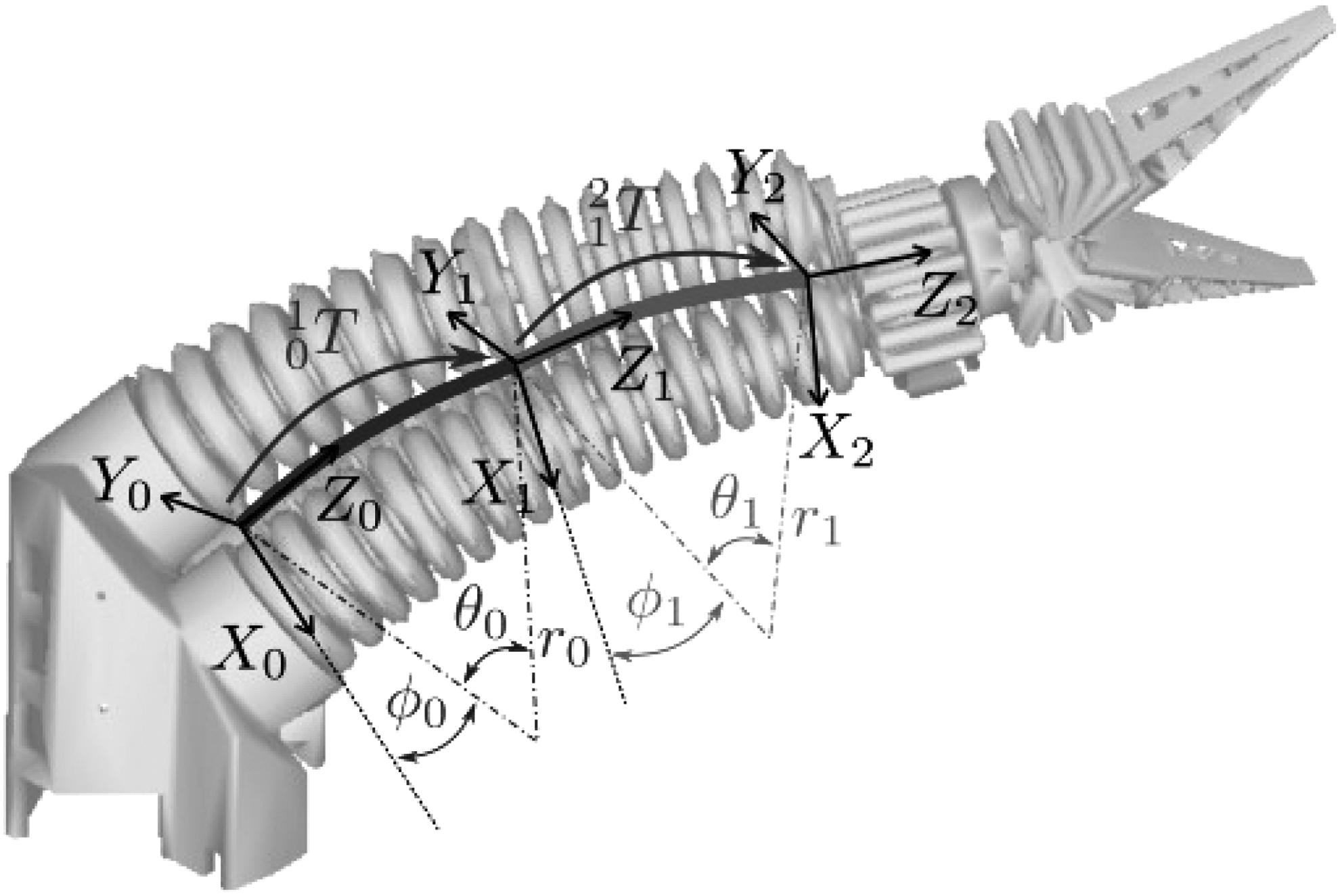
In this approach, developed in detail in Ref.³⁴ the CBHA is considered 17 vertebrae serially connected. Between each pair of vertebrae, an intervertebra section is modeled as a 3UPS-1UP joint (3 universal-prismatic-spherical joints and one universal-prismatic joint). The behavior of a substructure composed by two vertebrae and an intervertebra is represented by a parallel robot with three DoFs, as shown in Figure 7.

FIG. 7.

Substructure of the CBHA modeled as a parallel robot.

The parallel robot consists of an upper and a lower platform connected by three limbs and a central leg. The limbs are modeled by a UPS joint in which only the prismatic part is active, allowing the control of the position and orientation of the upper vertebra, with respect to the lower vertebra. The central leg is modeled as a passive UP joint and is used to constraint the rotation about the longitudinal axis of the parallel robot, as well as any shearing motion between the vertebrae.

The position and orientation of the upper vertebra k + 1, with respect to the lower vertebra k, are given by the transformation matrix: \documentclass{aastex}\usepackage{amsbsy}\usepackage{amsfonts}\usepackage{amssymb}\usepackage{bm}\usepackage{mathrsfs}\usepackage{pifont}\usepackage{stmaryrd}\usepackage{textcomp}\usepackage{portland, xspace}\usepackage{amsmath, amsxtra}\usepackage{upgreek}\pagestyle{empty}\DeclareMathSizes{10}{9}{7}{6}\begin{document} \begin{align*} _{{ \rm{k}} + { \rm{1}}}^{ \rm{k}}{ \rm{T}} = \left[ { \begin{matrix} {c{ \theta _k}} & {s{ \theta _k}s{ \psi _k}} & {s{ \theta _k}c{ \psi _k}} & 0 \\ 0 & {c{ \psi _k}} & { - s{ \psi _k}} & 0 \\ { - s{ \theta _k}} & {s{ \psi _k}c{ \theta _k}} & {c{ \theta _k}c{ \psi _k}} & {{z_k}} \\ 0 & 0 & 0 & 1 \\ \end{matrix} } \right] , \tag{19} \end{align*} \end{document}

where the angles θ_k and ψ_k represent pitch and roll angles, respectively, and the notations s and c mean sine and cosine, respectively. In this model, the prismatic variable q_n,k shown in Figure 7 represents the length of each intervertebra, which is a percentage of the total length of the actuator. This percentage can be obtained by considering the minimum and maximum elongation of each intervertebra. This development is presented in detail in Ref.³⁴

Experimental validation and model comparison

To validate the model, a set of 50 end-effector positions distributed inside the task space of the manipulator were selected. For each position, the correspondent configuration of the robot was recorded using the string potentiometers that are placed along the structure of the robot. The set of lengths recorded were used as an input for the FKM. The experiment assumes zero end-effector payload. The results are compared with those of the constant curvature and the hybrid approach. This comparison is presented in Figures 8 and 9.

FIG. 8.

x/y View of the results from the model comparison. FEM, finite element method. Color images available online at www.liebertpub.com/soro

FIG. 9.

x/z View of the results from the model comparison. Color images available online at www.liebertpub.com/soro

The results show that the constraint approach is more accurate in estimating the position of the end-effector, with a root-mean-square error of 4.66 mm, compared with 12.87 and 17.09 mm of error for the constant curvature and the hybrid approaches, respectively. We hypothesize that the imprecise measurement of displacement for each vertebra may be the cause of the hybrid approach being less precise than ours, as there were only six string potentiometers available to chart the displacements. Moreover, this model was initially developed to be able to inverse it, more than for the pure precision of the FKM.

Nevertheless, the FEM model still has a few limitations in its development. These limitations represent the main source of error in the results: for the moment, the constitutive law used to model the material of the trunk is only an approximation. Moreover, nonlinear effects like the viscosity of the material are not yet implemented in the model.

Another source of error comes from the geometry of the trunk itself. When the trunk is bent at a maximum angle, the outer walls of the pneumatic cavities collide with each other, as shown in Figure 10. The consideration of these collisions is not yet implemented in the simulation.

FIG. 10.

Collision of the outer wall of the cavities. The collisions occur on the orange edges depicted in the bent actuator (right). Color images available online at www.liebertpub.com/soro

The generic nature of the approach showcased in this article is illustrated by obtaining the inverse kinematics of two different soft manipulators. The simulation of the inverse model provides the position control of the robots in open loop, which can be used to pilot directly the robot, as in the case of the parallel soft robot.

Inverse kinematic model

In this section, an experimental validation of the modeling methodology is conducted using two different soft robots:

A parallel soft robot made of silicone, actuated with tendons (cables) controlled in position, and

The CBHA.

The inverse model provided by convex optimization in real time allows to teleoperate the robots in open loop: given a desired input position of the effector, the desired output for the actuators is computed. For the soft parallel robot, a desired position of the tendons is provided.

Modeling and feed-forward control of a parallel soft robot

This experiment is based on a 3D soft robot, made of silicone, the design of which is inspired by parallel robots with closed kinematic chains (Fig. 11). In its rest position, the dimensions of the robot are 180 × 180 × 130 mm. The robot naturally deforms and sinks under the action of gravity, but four unilateral actuators (servomotors that are connected to the structure of the robot with cables) are placed on each leg to prevent and pilot the deformation. The effector position is placed on the upper part of the robot. Its trajectory is defined in 3D (and can interactively be changed by a user) and the algorithm provides the position to apply to the servomotors. The Young's modulus of the silicone, measured experimentally, is used to parameterize the robot. The FEM model of the robot is composed of 4147 tetrahedrons and 1628 nodes. When projected in the constraint space, the size of the system is highly reduced: three equations for the effector and four equations for the actuators. The convex optimization that leads to the inverse model can be performed in real time. The most time-expensive part of the computation is the projection expressed in Equations (7) and (8) (50 ms on a Core i7, 2.8 GHz), but when using the graphics processing unit method described in Ref.³⁵ it significantly reduces the computation time of the projection (15 ms in this case).

FIG. 11.

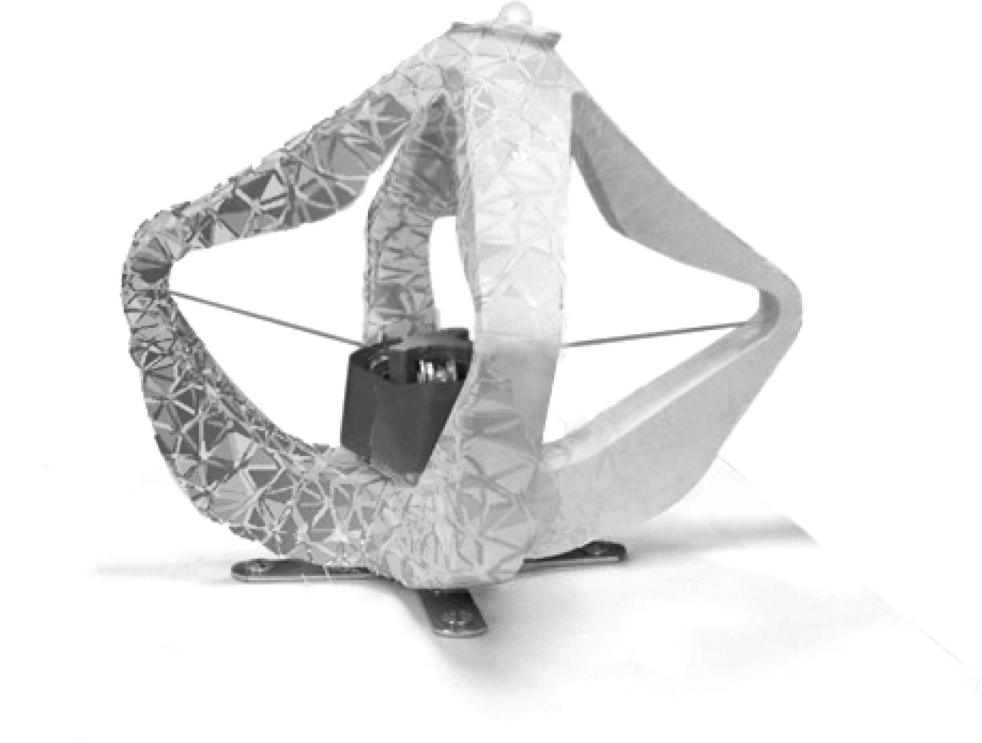
Deformable parallel manipulator.

To validate the method, a study of the discrepancy between the desired positions and the obtained positions is conducted on static positions distributed across a workspace of 25 × 25 × 50 mm around the rest position of the robot as shown in Figure 12. The measurements are performed using a motion capture system based on infrared cameras.^‡ On a sample of 28 positions, a mean error of 1.4 mm is obtained with a standard deviation of 0.6 mm and a maximum error of 2.9 mm. This illustrates the precision that can be achieved using such FEM approaches.

FIG. 12.

Comparison of desired trajectory and measured trajectory of the parallel manipulator. Color images available online at www.liebertpub.com/soro

It can be noted that these results are obtained by using an open loop and with a position to position control: for a given position of the effector, the algorithm finds a position for the actuator cables. This is a favorable case for FEM precision because the partial differential equations are enforced with Dirichlet boundary conditions.

Inverse kinematics of the CBHA

Considering the kinematic relationship for the CBHA given in the section Forward kinematic models, that is the link between the actuator lengths and the position of the end-effector, the IKM, solved by the convex optimization, will give the actuator lengths that result from a predefined end-effector position. The FEM analysis applied to model this soft robot is detailed in Ref.³⁶ A domain decomposition strategy is applied to perform the computation of the model (Eq. 3) and the projection in the constraint space (Eq. 7). After the actuator contribution required to achieve the desired position of the end-effector is applied to the model, and the position of the nodes is updated, the readings from the sensors in the simulation, given by Equation (6), will give the lengths of the pneumatic actuators that represent the output of the IKM.

To validate the method, a set of 50 end-effector positions is selected inside the task space of the robot and the corresponding set of lengths for each position is recorded by the sensors of the robot. The same set of positions is used as inputs for the inverse model, and the resultant length of each actuator is estimated. This study is summarized in Table 1, where l₁,…, l₆ represent the lengths of the actuators and their values are in mm, μ represents the mean error, and σ is the standard deviation. The results are presented in Figure 13.

FIG. 13.

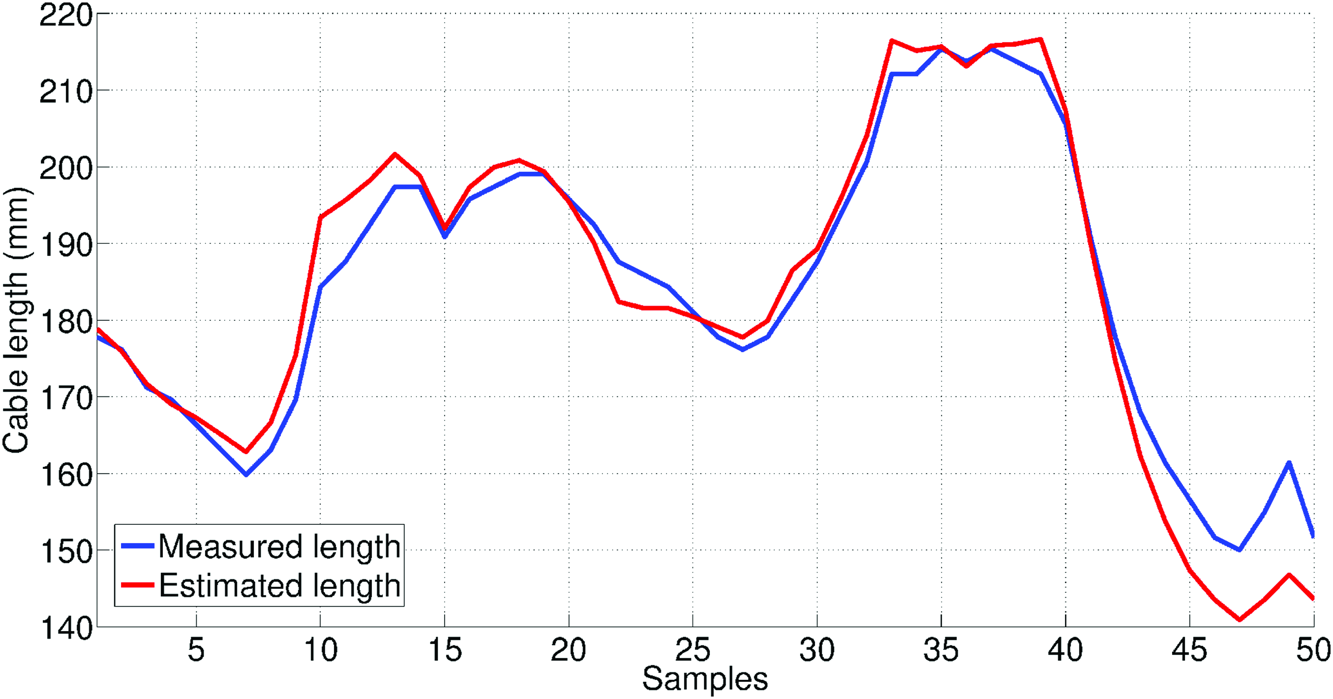
Comparison of measured and estimated lengths of one of the sensors, given a predefined set of end-effector positions for the CBHA. Color images available online at www.liebertpub.com/soro

Table 1.

Statistical Analysis of the Error Between Measured and Estimated Lengths for the Compact Bionic Handling Assistant

l (mm)	l₁	l₂	l₃	l₄	l₅	l₆
μ (mm)	3.2	2.43	3.86	4.08	3.6	3.69
σ (mm)	1.55	1.76	2.05	2.12	2.56	2.06

The results show a mean error between 2.43 and 4.08 mm across all lengths, which represents between 1.21% and 2.04% of the total length of the manipulator. As in the case of the parallel robot, the set of actuator contributions (in this case, the pressures applied to the cavities) obtained from the optimization process can be used as input for the real robot to obtain a feed-forward control. However, as explained before, there are some considerable discrepancies between the pressure calculated by the simulation and the pressure applied to the cavities, mainly caused by the way the pressure is regulated in the robot. This leads to less accurate results.

To improve the results in terms of efforts (pressure and force) in the inverse model, one can use more advanced constitutive models for the materials. One of these models is the St. Venant–Kirchhoff hyperelastic model. The stress/strain relationship in the St. Venant–Kirchhoff model is represented by the second Piola–Kirchhoff stress tensor S that has the following form: \documentclass{aastex}\usepackage{amsbsy}\usepackage{amsfonts}\usepackage{amssymb}\usepackage{bm}\usepackage{mathrsfs}\usepackage{pifont}\usepackage{stmaryrd}\usepackage{textcomp}\usepackage{portland, xspace}\usepackage{amsmath, amsxtra}\usepackage{upgreek}\pagestyle{empty}\DeclareMathSizes{10}{9}{7}{6}\begin{document} \begin{align*} { \bf{S}} = \lambda \ { \bf{tr}} ( { \bf{E}} ) { \bf{I}} + 2 \mu \ { \bf{E}} , \tag{20} \end{align*} \end{document}

where E is the Lagrange–Green strain tensor and λ and μ are the Lamé constants that can be approximated from the Young's modulus and Poisson's ratio of the material in question. We have conducted tests on the parallel soft robot using the St. Venant–Kirchhoff model to compare the results to those obtained using the corotational formulation. In the tests, we observed very small errors in the displacement output (3.24% of a total cable stroke of 50 mm). In case of the force output, we observed bigger errors (16.02% of the tension in the cable) related to the errors made by the corotational formulation in the stress computation.

Deflection of end-effector under external loading

As explained in the Methods section, one of the advantages of this modeling approach is the ability to predict the deflection of the robot under external loading, given a good representation of the material mechanics. If the load is known a priori, the value of the force acting on the end-effector λ_e can be used in Equation (3) to compute the position that accounts for said force. To validate this modeling feature, a set of experiments was conducted on both manipulators using known loads.

First, an initial configuration for the manipulator without loading is selected and the position of the end-effector is measured, then the load is applied and the new position of the end-effector is recovered after the robot achieves static equilibrium. The same load is then applied to the model of the manipulator using the same initial pose and the resulting end-effector position is also recovered. In the case of the CBHA, the model of the sensors presented in the Sensor Constraint Model section is used to apply the configuration of the real robot measured by the string potentiometers to the simulation model. A vector that connects initial and final end-effector positions represents the deflection caused by the loading.

To assess the repeatability of the measurements, the loading sequence described before is performed 40 times for each loading value and the average value is then used for the model validation. A standard deviation of 0.4838 mm is obtained across all the measurements. The comparison between measured and model deflections for both manipulators is presented in Figures 14 and 15.

FIG. 14.

Comparison between measured and predicted deflections caused by external loading on the parallel manipulator. Color images available online at www.liebertpub.com/soro

FIG. 15.

Comparison between measured and predicted deflections caused by external loading on the CBHA manipulator. Color images available online at www.liebertpub.com/soro

In the figures, the blue line represents the compliance to loading of the manipulators and the red line is the prediction of the model. In the case of the CBHA, the maximum error is 4.107 mm, with an average error of 2.1047 mm. Nevertheless, Figure 15 shows that the CBHA presents strain hardening/necking stages of plastic behavior at the beginning of the loading profile, which corresponds to the compliance of the plastic material from which the manipulator is made of (polyamide nylon), and therefore the model prediction is accurate only for a small region of the profile. To improve the model predictive capabilities for the CBHA in particular, two constitutive laws could be implemented to account for the different behaviors, but this would modify the way the inverse FEM is formulated. In contrast, the maximum error in the case of the parallel manipulator is 2.06 mm with an average error of 2.01 mm. The reason we obtain better results is because the material of the parallel robot conforms better to the assumption of high deformation and low stress, while also being an elastic material with no plastic behavior.

FEM-Based Closed-Loop Control of Continuum Robots

In the Inverse Kinematics of the CBHA section, the relationship between the sensor lengths and the end-effector position of the CBHA was obtained based on the FEM simulation of the robot; however, to control the motion of the robot, the set of pressures applied to the actuators is to be computed. Indeed, the relationship given by Equation (7) can be used to control directly the robot in open loop, but as explained in the Forward Kinematic Model section, this requires an accurate control over the pressures applied to the robot. Moreover, nonlinear behaviors like the hysteresis and strain-rate dependency of the material (which is not considered in the model) render the feed-forward control of the manipulators unusable in real applications.

Controllers for soft manipulators have been investigated in the past with the intention of rejecting nonlinear behaviors and model uncertainties that result from the complex dynamics of the manipulators. Control based on energy formulations,³⁷ model-less approaches,³⁸ and feedback controllers^39,40 has been proposed before with the intention of achieving accurate positioning of the manipulators in the presence of nonmodeled dynamics. In this section, a closed-loop control strategy based on a state estimator is proposed.

Closed-loop control design

The closed-loop controller is designed to ensure the correct configuration of the robot, given a desired end-effector position. A reference computation is performed to transform the desired position to the correspondent configuration. Assuming that the external forces are constant, the discrete model of the system, derived form of Equation (9), takes the following form: \documentclass{aastex}\usepackage{amsbsy}\usepackage{amsfonts}\usepackage{amssymb}\usepackage{bm}\usepackage{mathrsfs}\usepackage{pifont}\usepackage{stmaryrd}\usepackage{textcomp}\usepackage{portland, xspace}\usepackage{amsmath, amsxtra}\usepackage{upgreek}\pagestyle{empty}\DeclareMathSizes{10}{9}{7}{6}\begin{document} \begin{align*} { \delta _{s , k + 1}} = { \delta _{s , k}} + {{ \bf{J}}_{sa}} ( {{ \bf{x}}_k} ) \Delta { \lambda _{a , k + { \bf{1}}}} , \tag{21} \end{align*} \end{document}

where J_sa = W_sa is the Jacobian matrix between sensors and actuators. When the desired sensor lengths are provided by the reference computation, we can propose the closed-loop control approach shown in Figure 16.

FIG. 16.

Closed-loop control of the CBHA based on IKM and FKM simultaneous simulations and the controller. FKM, forward kinematic model; IKM, inverse kinematic model.

In Figure 16, the blue blocks represent the computations performed by simulation. Two simulations executing simultaneously are implemented in the closed-loop system: one main simulation that computes the IKM and a second simulation that acts as a state estimator for the system. The state estimator is the FKM simulation of the robot that computes an estimated configuration for the robot based on the lengths of the sensors. This configuration is used to update the state of the IKM at each simulation step. In this way, we make sure that the configurations of both simulation model and the manipulator are similar before the estimation of the Jacobian is computed. The tracking error e_k in the closed-loop system is computed as follows: \documentclass{aastex}\usepackage{amsbsy}\usepackage{amsfonts}\usepackage{amssymb}\usepackage{bm}\usepackage{mathrsfs}\usepackage{pifont}\usepackage{stmaryrd}\usepackage{textcomp}\usepackage{portland, xspace}\usepackage{amsmath, amsxtra}\usepackage{upgreek}\pagestyle{empty}\DeclareMathSizes{10}{9}{7}{6}\begin{document} \begin{align*} {e_k} = { \delta _{s , k}} - \delta _{s , k}^d , \tag{22} \end{align*} \end{document}

where \documentclass{aastex}\usepackage{amsbsy}\usepackage{amsfonts}\usepackage{amssymb}\usepackage{bm}\usepackage{mathrsfs}\usepackage{pifont}\usepackage{stmaryrd}\usepackage{textcomp}\usepackage{portland, xspace}\usepackage{amsmath, amsxtra}\usepackage{upgreek}\pagestyle{empty}\DeclareMathSizes{10}{9}{7}{6}\begin{document} $$\delta _{s , k}^d$$ \end{document} represents the desired lengths of the sensors and δ_s,k represents the current lengths in the robot. We define the control vector v_k as follows: \documentclass{aastex}\usepackage{amsbsy}\usepackage{amsfonts}\usepackage{amssymb}\usepackage{bm}\usepackage{mathrsfs}\usepackage{pifont}\usepackage{stmaryrd}\usepackage{textcomp}\usepackage{portland, xspace}\usepackage{amsmath, amsxtra}\usepackage{upgreek}\pagestyle{empty}\DeclareMathSizes{10}{9}{7}{6}\begin{document} \begin{align*} {{ \bf{v}}_k} = {{ \bf{ \hat { J}}}_{sa}} ( {{ \bf{ \hat { x}}}_k} ) {{ \bf{r}}_k} , \tag{23} \end{align*} \end{document}

where \documentclass{aastex}\usepackage{amsbsy}\usepackage{amsfonts}\usepackage{amssymb}\usepackage{bm}\usepackage{mathrsfs}\usepackage{pifont}\usepackage{stmaryrd}\usepackage{textcomp}\usepackage{portland, xspace}\usepackage{amsmath, amsxtra}\usepackage{upgreek}\pagestyle{empty}\DeclareMathSizes{10}{9}{7}{6}\begin{document} $${{ \bf{ \hat { J}}}_{sa}} ( {{ \bf{ \hat { x}}}_k} )$$ \end{document} is the estimated Jacobian matrix between the sensors and actuators, and r_k = Δλ_a_,k+1. Using Equation (23), the kinematic model can be rewritten as follows: \documentclass{aastex}\usepackage{amsbsy}\usepackage{amsfonts}\usepackage{amssymb}\usepackage{bm}\usepackage{mathrsfs}\usepackage{pifont}\usepackage{stmaryrd}\usepackage{textcomp}\usepackage{portland, xspace}\usepackage{amsmath, amsxtra}\usepackage{upgreek}\pagestyle{empty}\DeclareMathSizes{10}{9}{7}{6}\begin{document} \begin{align*} { \delta _{s , k + 1}} = { \delta _{s , k}} + {{ \bf{v}}_k} \tag{24} \end{align*} \end{document}

The control law is based on proportional integrative strategy; therefore, the control vector v_k is designed in the sensor space as follows: \documentclass{aastex}\usepackage{amsbsy}\usepackage{amsfonts}\usepackage{amssymb}\usepackage{bm}\usepackage{mathrsfs}\usepackage{pifont}\usepackage{stmaryrd}\usepackage{textcomp}\usepackage{portland, xspace}\usepackage{amsmath, amsxtra}\usepackage{upgreek}\pagestyle{empty}\DeclareMathSizes{10}{9}{7}{6}\begin{document} \begin{align*} {{ \bf{v}}_k} = - {k_p}{e_k} - {k_i}{h_k} , \tag{25} \end{align*} \end{document}

where k_p and k_i are the proportional and integrative gains of the controller, respectively. The integrative term h at time k + 1 is computed as \documentclass{aastex}\usepackage{amsbsy}\usepackage{amsfonts}\usepackage{amssymb}\usepackage{bm}\usepackage{mathrsfs}\usepackage{pifont}\usepackage{stmaryrd}\usepackage{textcomp}\usepackage{portland, xspace}\usepackage{amsmath, amsxtra}\usepackage{upgreek}\pagestyle{empty}\DeclareMathSizes{10}{9}{7}{6}\begin{document} \begin{align*} {h_{k + 1}} = {h_k} + {e_k} \tag{26} \end{align*} \end{document}

Then, the control allocation based on a QP formulation⁴¹ is employed to find a unique solution to \documentclass{aastex}\usepackage{amsbsy}\usepackage{amsfonts}\usepackage{amssymb}\usepackage{bm}\usepackage{mathrsfs}\usepackage{pifont}\usepackage{stmaryrd}\usepackage{textcomp}\usepackage{portland, xspace}\usepackage{amsmath, amsxtra}\usepackage{upgreek}\pagestyle{empty}\DeclareMathSizes{10}{9}{7}{6}\begin{document} \begin{align*} {{ \bf{r}}_k} = { \bf{ \hat { J}}}_{sa}^ + ( {{ \bf{ \hat { x}}}_k} ) {{ \bf{v}}_k} , \tag{27} \end{align*} \end{document}

where \documentclass{aastex}\usepackage{amsbsy}\usepackage{amsfonts}\usepackage{amssymb}\usepackage{bm}\usepackage{mathrsfs}\usepackage{pifont}\usepackage{stmaryrd}\usepackage{textcomp}\usepackage{portland, xspace}\usepackage{amsmath, amsxtra}\usepackage{upgreek}\pagestyle{empty}\DeclareMathSizes{10}{9}{7}{6}\begin{document} $${ \bf{ \hat { J}}}_{sa}^ +$$ \end{document} is the pseudo-inverse of the estimated Jacobian. In practice, as \documentclass{aastex}\usepackage{amsbsy}\usepackage{amsfonts}\usepackage{amssymb}\usepackage{bm}\usepackage{mathrsfs}\usepackage{pifont}\usepackage{stmaryrd}\usepackage{textcomp}\usepackage{portland, xspace}\usepackage{amsmath, amsxtra}\usepackage{upgreek}\pagestyle{empty}\DeclareMathSizes{10}{9}{7}{6}\begin{document} $${{ \bf{ \hat { J}}}_{sa}} ( {{ \bf{ \hat { x}}}_k} )$$ \end{document} may not be fully invertible, we introduce a variable O defined as \documentclass{aastex}\usepackage{amsbsy}\usepackage{amsfonts}\usepackage{amssymb}\usepackage{bm}\usepackage{mathrsfs}\usepackage{pifont}\usepackage{stmaryrd}\usepackage{textcomp}\usepackage{portland, xspace}\usepackage{amsmath, amsxtra}\usepackage{upgreek}\pagestyle{empty}\DeclareMathSizes{10}{9}{7}{6}\begin{document} \begin{align*} O = { \bf{ \hat { J}}}_{sa}^ + ( {{ \bf{ \hat { x}}}_k} ) {{ \bf{r}}_k} - {{ \bf{v}}_k} \tag{28} \end{align*} \end{document}

Using O, the QP problem formulation (the Inverse Model by Convex Optimization section) becomes \documentclass{aastex}\usepackage{amsbsy}\usepackage{amsfonts}\usepackage{amssymb}\usepackage{bm}\usepackage{mathrsfs}\usepackage{pifont}\usepackage{stmaryrd}\usepackage{textcomp}\usepackage{portland, xspace}\usepackage{amsmath, amsxtra}\usepackage{upgreek}\pagestyle{empty}\DeclareMathSizes{10}{9}{7}{6}\begin{document} \begin{align*} \mathop { \min } \limits_{{{ \bf{u}}_k}} \quad ( {O^T}O ) , \tag{29} \end{align*} \end{document}

the resulting r_k will be the best possible inversion of Equation (23) in the least square sense. In addition, the QP formulation allows to define constraints like actuator saturation or positive direction of actuation. Using Equation (25 in Eq. 27), r_k is rewritten as follows: \documentclass{aastex}\usepackage{amsbsy}\usepackage{amsfonts}\usepackage{amssymb}\usepackage{bm}\usepackage{mathrsfs}\usepackage{pifont}\usepackage{stmaryrd}\usepackage{textcomp}\usepackage{portland, xspace}\usepackage{amsmath, amsxtra}\usepackage{upgreek}\pagestyle{empty}\DeclareMathSizes{10}{9}{7}{6}\begin{document} \begin{align*} {{ \bf{r}}_k} = - { \bf{ \hat { J}}}_{sa}^ + ( {{ \bf{ \hat { x}}}_k} ) ( {k_p}{e_k} + {k_i}{h_k} ) \tag{30} \end{align*} \end{document}

Using Equation (30 in Eq. 21), the closed-loop system is defined as \documentclass{aastex}\usepackage{amsbsy}\usepackage{amsfonts}\usepackage{amssymb}\usepackage{bm}\usepackage{mathrsfs}\usepackage{pifont}\usepackage{stmaryrd}\usepackage{textcomp}\usepackage{portland, xspace}\usepackage{amsmath, amsxtra}\usepackage{upgreek}\pagestyle{empty}\DeclareMathSizes{10}{9}{7}{6}\begin{document} \begin{align*} {e_{k + 1}} = {e_k} + {{ \bf{J}}_{sa}} ( {{ \bf{x}}_k} ) {{ \bf{r}}_k} , \tag{31} \end{align*} \end{document}

which in the ideal case in which \documentclass{aastex}\usepackage{amsbsy}\usepackage{amsfonts}\usepackage{amssymb}\usepackage{bm}\usepackage{mathrsfs}\usepackage{pifont}\usepackage{stmaryrd}\usepackage{textcomp}\usepackage{portland, xspace}\usepackage{amsmath, amsxtra}\usepackage{upgreek}\pagestyle{empty}\DeclareMathSizes{10}{9}{7}{6}\begin{document} $${{ \bf{ \hat { J}}}_{sa}}$$ \end{document} is invertible, and can be written as follows: \documentclass{aastex}\usepackage{amsbsy}\usepackage{amsfonts}\usepackage{amssymb}\usepackage{bm}\usepackage{mathrsfs}\usepackage{pifont}\usepackage{stmaryrd}\usepackage{textcomp}\usepackage{portland, xspace}\usepackage{amsmath, amsxtra}\usepackage{upgreek}\pagestyle{empty}\DeclareMathSizes{10}{9}{7}{6}\begin{document} \begin{align*} {e_{k + 1}} = {e_k} + {{ \bf{v}}_k} \tag{32} \end{align*} \end{document}

The system of Equation (32) is a simple first-order discrete model that can be controlled with any standard controller. We choose the control strategy to be based on proportional-integrative control law because we want to improve the convergence rate and remove any steady state error (in the sensor space at least). After testing, the selected gain values are k_p = 0.14 and k_i = 0.0003, as a compromise between the rise time of the signal and its overshot. Figure 17 shows the response of one actuator length of the simulated robot and the real robot, given a precomputed set points corresponding to an end-effector position inside the task space of the robot. The position is chosen so that the actuators are far from their saturation points. The model simulation and the real robot have different initial condition. The experiment was performed for 2500 simulation steps with a simulation step of 0.1 s. After 1000 simulation steps, the set points are changed in both the simulation and the real robot.

FIG. 17.

Comparison of real and estimated actuator length of the CBHA. A second set point is applied to the system after 1000 simulation steps to observe the performance of the controller. The time step is 0.1 s for the experiment. Color images available online at www.liebertpub.com/soro

The results show that both, the simulation of the robot and the robot itself, have the same settling time, t_s ≈ 400 simulation steps. We can also see that the curve that represents the measured value of the lengths in the robot jumps between two values. This behavior is a consequence of the poor resolution of the string potentiometers. Figure 17 also shows a different behavior in the transitory stage of the curve of measured lengths. This behavior can be attributed to different factors: first, there is the time required to compute the configuration of the manipulator from the measured sensor lengths; second, there is a time delay for the desired pressure to be applied to the robot, and finally, the plasticity of the material from which the manipulator is built (polyamide-nylon), which is not accounted for in our FEM model. On the other hand, the pneumatic valves that control the pressure inside the actuators have a small dead zone; so, when the manipulator starts its motion from a zero-pressure condition, very small increments in the pressure do not produce any motion until this dead zone is surpassed, which is not considered in the FEM.

A second experiment was performed using the real robot in the loop. In this experiment, an external unknown force was applied to the manipulator to see the uncertainty rejection capabilities of the controller. Figure 18 shows the results of this experiment.

FIG. 18.

Measured lengths of the CBHA in closedloop. An external force is applied to the manipulator after 1050 time steps. The time step is 0.1 s for the experiment. Color images available online at www.liebertpub.com/soro

Robustness analysis

Because of modeling uncertainties, the estimated Jacobian matrix \documentclass{aastex}\usepackage{amsbsy}\usepackage{amsfonts}\usepackage{amssymb}\usepackage{bm}\usepackage{mathrsfs}\usepackage{pifont}\usepackage{stmaryrd}\usepackage{textcomp}\usepackage{portland, xspace}\usepackage{amsmath, amsxtra}\usepackage{upgreek}\pagestyle{empty}\DeclareMathSizes{10}{9}{7}{6}\begin{document} $${{ \bf{ \hat { J}}}_{sa}} ( {{ \bf{ \hat { x}}}_k} )$$ \end{document} is, in general, different from the Jacobian of the robot \documentclass{aastex}\usepackage{amsbsy}\usepackage{amsfonts}\usepackage{amssymb}\usepackage{bm}\usepackage{mathrsfs}\usepackage{pifont}\usepackage{stmaryrd}\usepackage{textcomp}\usepackage{portland, xspace}\usepackage{amsmath, amsxtra}\usepackage{upgreek}\pagestyle{empty}\DeclareMathSizes{10}{9}{7}{6}\begin{document} $${J_{sa}} ( {{\bf x}_k} )$$ \end{document} . We introduce the vector ω_k that represents the disparities between the real Jacobian and the estimated Jacobian. We call this vector the inversion error and is defined as follows: \documentclass{aastex}\usepackage{amsbsy}\usepackage{amsfonts}\usepackage{amssymb}\usepackage{bm}\usepackage{mathrsfs}\usepackage{pifont}\usepackage{stmaryrd}\usepackage{textcomp}\usepackage{portland, xspace}\usepackage{amsmath, amsxtra}\usepackage{upgreek}\pagestyle{empty}\DeclareMathSizes{10}{9}{7}{6}\begin{document} \begin{align*} { \omega _k} = [ { \bf{I}} - {{ \bf{J}}_{sa}} ( {{ \bf{x}}_{ \bf{k}}} ) { \bf{ \hat { J}}}_{sa}^ + ( {{ \bf{ \hat { x}}}_k} ) ] {{ \bf{v}}_k} \tag{33} \end{align*} \end{document}

Then, the closed-loop system is rewritten as follows: \documentclass{aastex}\usepackage{amsbsy}\usepackage{amsfonts}\usepackage{amssymb}\usepackage{bm}\usepackage{mathrsfs}\usepackage{pifont}\usepackage{stmaryrd}\usepackage{textcomp}\usepackage{portland, xspace}\usepackage{amsmath, amsxtra}\usepackage{upgreek}\pagestyle{empty}\DeclareMathSizes{10}{9}{7}{6}\begin{document} \begin{align*} {e_{k + 1}} = {e_k} + {{ \bf{v}}_k} + { \omega _k} = {e_k} - {k_p}{e_k} - {k_i}{h_k} + { \omega _k} \tag{34} \end{align*} \end{document}

The disturbed closed-loop system is \documentclass{aastex}\usepackage{amsbsy}\usepackage{amsfonts}\usepackage{amssymb}\usepackage{bm}\usepackage{mathrsfs}\usepackage{pifont}\usepackage{stmaryrd}\usepackage{textcomp}\usepackage{portland, xspace}\usepackage{amsmath, amsxtra}\usepackage{upgreek}\pagestyle{empty}\DeclareMathSizes{10}{9}{7}{6}\begin{document} \begin{align*} \left[ { \begin{matrix} {{e_{k + 1}}} \\ {{h_{k + 1}}} \\ {} \\ \end{matrix} } \right] = \left[ { \begin{matrix} {{ \bf{I}} - {k_p}{ \bf{I}}} & { - {k_i}{ \bf{I}}} \\ { \bf{I}} & { \bf{I}} \\ {} & {} \\ \end{matrix} } \right] \left[ { \begin{matrix} {{e_k}} \\ {{h_k}} \\ {} \\ \end{matrix} } \right] + \left[ { \begin{matrix} { \bf{I}} \\ 0 \\ {} \\ \end{matrix} } \right] { \omega _k} \tag{35} \end{align*} \end{document}

It can be disturbing that we end up with such a simple linear system. We emphasize to the reader that the nonlinearities are taken into account by the two simulation blocks (FKM and IKM in Fig. 16) in the closed-loop control. In Equation (35), we are writing the system in terms of e_k and h_k, and if the model was perfect, the system would be trivial. However, we can have modeling errors, which is why, in the following, we will prove that the control is robust to these modeling uncertainties ω_k.

To simplify the notation of the problem, we define the following vectors: \documentclass{aastex}\usepackage{amsbsy}\usepackage{amsfonts}\usepackage{amssymb}\usepackage{bm}\usepackage{mathrsfs}\usepackage{pifont}\usepackage{stmaryrd}\usepackage{textcomp}\usepackage{portland, xspace}\usepackage{amsmath, amsxtra}\usepackage{upgreek}\pagestyle{empty}\DeclareMathSizes{10}{9}{7}{6}\begin{document} \begin{align*} {{ \bf{X}}_{k + 1}} = \left[ { \begin{matrix} {{e_{k + 1}}} \\ {{h_{k + 1}}} \\ {} \\ \end{matrix} } \right] , {{ \bf{X}}_k} = \left[ { \begin{matrix} {{e_k}} \\ {{h_k}} \\ {} \\ \end{matrix} } \right] , { \bf{D}} = \left[ { \begin{matrix} { \bf{I}} \\ 0 \\ {} \\ \end{matrix} } \right] , { \bf{F}} = \left[ { \begin{matrix} {{k_p}} & {{k_i}} \\ {} & {} \\ \end{matrix} } \right] \tag{36} \end{align*} \end{document}

Also, \documentclass{aastex}\usepackage{amsbsy}\usepackage{amsfonts}\usepackage{amssymb}\usepackage{bm}\usepackage{mathrsfs}\usepackage{pifont}\usepackage{stmaryrd}\usepackage{textcomp}\usepackage{portland, xspace}\usepackage{amsmath, amsxtra}\usepackage{upgreek}\pagestyle{empty}\DeclareMathSizes{10}{9}{7}{6}\begin{document} \begin{align*} \left[ { \begin{matrix} {{ \bf{I}} - {k_p}{ \bf{I}}} & { - {k_i}{ \bf{I}}} \\ { \bf{I}} & { \bf{I}} \\ {} & {} \\ \end{matrix} } \right] = { \bf{A}} - { \bf{BF}} , \tag{37} \end{align*} \end{document}

Using this notation, matrix ω_k is written as follows: \documentclass{aastex}\usepackage{amsbsy}\usepackage{amsfonts}\usepackage{amssymb}\usepackage{bm}\usepackage{mathrsfs}\usepackage{pifont}\usepackage{stmaryrd}\usepackage{textcomp}\usepackage{portland, xspace}\usepackage{amsmath, amsxtra}\usepackage{upgreek}\pagestyle{empty}\DeclareMathSizes{10}{9}{7}{6}\begin{document} \begin{align*} { \omega _k} = [ { \bf{I}} - {{ \bf{J}}_{sa}} ( {{ \bf{x}}_{ \bf{k}}} ) { \bf{ \hat { J}}}_{sa}^ + ( {{ \bf{ \hat { x}}}_k} ) ] { \bf{F}}{{ \bf{X}}_k} \tag{39} \end{align*} \end{document}

We assume that the error in the Jacobian estimation is bounded by a bounding parameter γ such that

\documentclass{aastex}\usepackage{amsbsy}\usepackage{amsfonts}\usepackage{amssymb}\usepackage{bm}\usepackage{mathrsfs}\usepackage{pifont}\usepackage{stmaryrd}\usepackage{textcomp}\usepackage{portland, xspace}\usepackage{amsmath, amsxtra}\usepackage{upgreek}\pagestyle{empty}\DeclareMathSizes{10}{9}{7}{6}\begin{document} \begin{align*} \omega _k^T{ \omega _k} = { \bf{X}}_k^T{{ \bf{F}}^T}{ [ { \bf{I}} - {{ \bf{J}}_{sa}} ( {{ \bf{x}}_{ \bf{k}}} ) { \bf{ \hat J}}_{sa}^ + ( {{ \bf{ \hat x}}_k} ) ] ^T} [ { \bf{I}} - {{ \bf{J}}_{sa}} ( {{ \bf{x}}_{ \bf{k}}} ) { \bf{ \hat J}}_{sa}^ + ( {{ \bf{ \hat x}}_k} ) ] { \bf{F}}{{ \bf{X}}_k} \le { \gamma ^2}{ \bf{X}}_k^T{{ \bf{F}}^T}{ \bf{F}}{{ \bf{X}}_k} , \tag{40}\end{align*} \end{document}

with \documentclass{aastex}\usepackage{amsbsy}\usepackage{amsfonts}\usepackage{amssymb}\usepackage{bm}\usepackage{mathrsfs}\usepackage{pifont}\usepackage{stmaryrd}\usepackage{textcomp}\usepackage{portland, xspace}\usepackage{amsmath, amsxtra}\usepackage{upgreek}\pagestyle{empty}\DeclareMathSizes{10}{9}{7}{6}\begin{document} \begin{align*} { [ { \bf{I}} - {{ \bf{J}}_{sa}} ( {{ \bf{x}}_{ \bf{k}}} ) { \bf{ \hat { J}}}_{sa}^ + ( {{ \bf{ \hat { x}}}_k} ) ] ^T} [ { \bf{I}} - {{ \bf{J}}_{sa}} ( {{ \bf{x}}_{ \bf{k}}} ) { \bf{ \hat { J}}}_{sa}^ + ( {{ \bf{ \hat { x}}}_k} ) ] \le { \gamma ^2}{ \bf{I}} \tag{41} \end{align*} \end{document}

For the proof of stability, we use Lyapunov's second method of stability.⁴² We define the Lyapunov candidate function as follows: \documentclass{aastex}\usepackage{amsbsy}\usepackage{amsfonts}\usepackage{amssymb}\usepackage{bm}\usepackage{mathrsfs}\usepackage{pifont}\usepackage{stmaryrd}\usepackage{textcomp}\usepackage{portland, xspace}\usepackage{amsmath, amsxtra}\usepackage{upgreek}\pagestyle{empty}\DeclareMathSizes{10}{9}{7}{6}\begin{document} \begin{align*} V = { \bf{X}}_k^T{ \bf{P}}{{ \bf{X}}_k} , \tag{42} \end{align*} \end{document}

where P is an unknown Lyapunov matrix with the properties \documentclass{aastex}\usepackage{amsbsy}\usepackage{amsfonts}\usepackage{amssymb}\usepackage{bm}\usepackage{mathrsfs}\usepackage{pifont}\usepackage{stmaryrd}\usepackage{textcomp}\usepackage{portland, xspace}\usepackage{amsmath, amsxtra}\usepackage{upgreek}\pagestyle{empty}\DeclareMathSizes{10}{9}{7}{6}\begin{document} \begin{align*} {{ \bf{P}}^T} = { \bf{P}} > 0 \tag{43} \end{align*} \end{document}

From Equation (42) and the notation given in Equation (36), the variation of the Lyapunov function is defined as follows: \documentclass{aastex}\usepackage{amsbsy}\usepackage{amsfonts}\usepackage{amssymb}\usepackage{bm}\usepackage{mathrsfs}\usepackage{pifont}\usepackage{stmaryrd}\usepackage{textcomp}\usepackage{portland, xspace}\usepackage{amsmath, amsxtra}\usepackage{upgreek}\pagestyle{empty}\DeclareMathSizes{10}{9}{7}{6}\begin{document} \begin{align*} \Delta V = { \bf{X}}_{k + 1}^T{ \bf{P}}{{ \bf{X}}_{k + 1}} - { \bf{X}}_k^T{ \bf{P}}{{ \bf{X}}_k} \tag{44} \end{align*} \end{document}

Using Equation (38), Equation (44) is redefined as follows: \documentclass{aastex}\usepackage{amsbsy}\usepackage{amsfonts}\usepackage{amssymb}\usepackage{bm}\usepackage{mathrsfs}\usepackage{pifont}\usepackage{stmaryrd}\usepackage{textcomp}\usepackage{portland, xspace}\usepackage{amsmath, amsxtra}\usepackage{upgreek}\pagestyle{empty}\DeclareMathSizes{10}{9}{7}{6}\begin{document} \begin{align*} \Delta V = ( ( { \bf{A}} - { \bf{BF}} ) {{ \bf{X}}_k} + { \bf{D}}{ \omega _k}{ ) ^T}{ \bf{P}} ( ( { \bf{A}} - { \bf{BF}} ) {{ \bf{X}}_k} + { \bf{D}}{ \omega _k} ) - { \bf{X}}_k^T{ \bf{P}}{{ \bf{X}}_k} \tag{45} \end{align*} \end{document}

By making \documentclass{aastex}\usepackage{amsbsy}\usepackage{amsfonts}\usepackage{amssymb}\usepackage{bm}\usepackage{mathrsfs}\usepackage{pifont}\usepackage{stmaryrd}\usepackage{textcomp}\usepackage{portland, xspace}\usepackage{amsmath, amsxtra}\usepackage{upgreek}\pagestyle{empty}\DeclareMathSizes{10}{9}{7}{6}\begin{document} \begin{align*} { \bf{A}} - { \bf{BF}} = { \bf{C}} , \tag{46} \end{align*} \end{document}

Equation (45) is written as follows: \documentclass{aastex}\usepackage{amsbsy}\usepackage{amsfonts}\usepackage{amssymb}\usepackage{bm}\usepackage{mathrsfs}\usepackage{pifont}\usepackage{stmaryrd}\usepackage{textcomp}\usepackage{portland, xspace}\usepackage{amsmath, amsxtra}\usepackage{upgreek}\pagestyle{empty}\DeclareMathSizes{10}{9}{7}{6}\begin{document} \begin{align*} { \Delta V} & { = ( { \bf{C}}{{ \bf{X}}_k} + { \bf{D}}{ \omega_k})^T{ \bf{P}} ( { \bf{C}}{{ \bf{X}}_k} + { \bf{D}}{ \omega _k} ) - { \bf{X}}_k^T{ \bf{P}}{{ \bf{X}}_k}} \\ & { = { \bf{X}}_k^T{{ \bf{C}}^T}{ \bf{PC}}{{ \bf{X}}_k} + { \bf{X}}_k^T{{ \bf{C}}^T}{ \bf{PD}}{ \omega _k} + \omega _k^T{{ \bf{D}}^T}{ \bf{PC}}{{ \bf{X}}_k}} \\ & \quad + \omega _k^T{{ \bf{D}}^T}{ \bf{PD}}{ \omega _k} - { \bf{X}}_k^T{ \bf{P}}{{ \bf{X}}_k} \tag{47}\end{align*} \end{document}

Reverting the notation in Equation (38), Equation (47) can be written in matrix form as follows: \documentclass{aastex}\usepackage{amsbsy}\usepackage{amsfonts}\usepackage{amssymb}\usepackage{bm}\usepackage{mathrsfs}\usepackage{pifont}\usepackage{stmaryrd}\usepackage{textcomp}\usepackage{portland, xspace}\usepackage{amsmath, amsxtra}\usepackage{upgreek}\pagestyle{empty}\DeclareMathSizes{10}{9}{7}{6}\begin{document} \begin{align*} \Delta V = { \left[ { \begin{matrix} {{{ \bf{X}}_k}} \\ {{ \omega _k}} \\ {} \\ \end{matrix} } \right] ^T} \left[ { \begin{matrix} {{{ ( { \bf{A}} - { \bf{BF}} ) }^T}{ \bf{P}} ( { \bf{A}} - { \bf{BF}} ) - { \bf{P}}} & {{{ ( { \bf{A}} - { \bf{BF}} ) }^T}{ \bf{PD}}} \\ {{{ \bf{D}}^T}{ \bf{P}} ( { \bf{A}} - { \bf{BF}} ) } & {{{ \bf{D}}^T}{ \bf{PD}}} \\ {} & {} \\ \end{matrix} } \right] \left[ { \begin{matrix} {{{ \bf{X}}_k}} \\ {{ \omega _k}} \\ {} \\ \end{matrix} } \right] \tag{48} \end{align*} \end{document}

For the proof, we introduce an accessory parameter α ≥ 0 in Equation (40), such that \documentclass{aastex}\usepackage{amsbsy}\usepackage{amsfonts}\usepackage{amssymb}\usepackage{bm}\usepackage{mathrsfs}\usepackage{pifont}\usepackage{stmaryrd}\usepackage{textcomp}\usepackage{portland, xspace}\usepackage{amsmath, amsxtra}\usepackage{upgreek}\pagestyle{empty}\DeclareMathSizes{10}{9}{7}{6}\begin{document} \begin{align*} \Upsilon = \alpha { \omega ^T} \omega - \alpha { \gamma ^2}{ \bf{X}}_k^T{{ \bf{F}}^T}{ \bf{F}}{{ \bf{X}}_k} < 0 \tag{49} \end{align*} \end{document}

From Equation (49), the left hand side of the inequality is written in matrix form as follows: \documentclass{aastex}\usepackage{amsbsy}\usepackage{amsfonts}\usepackage{amssymb}\usepackage{bm}\usepackage{mathrsfs}\usepackage{pifont}\usepackage{stmaryrd}\usepackage{textcomp}\usepackage{portland, xspace}\usepackage{amsmath, amsxtra}\usepackage{upgreek}\pagestyle{empty}\DeclareMathSizes{10}{9}{7}{6}\begin{document} \begin{align*} \Upsilon = { \left[ \begin{matrix} {{ \bf{X}}_k} \hfill \\ { \omega _k} \hfill \\\end{matrix} \right] ^T} \left[ { \begin{matrix} { - \alpha { \gamma ^2}{{ \bf{F}}^T}{ \bf{F}}} & 0 \\ 0 & { \alpha \ { \bf{I}}} \\ \end{matrix} } \right] \left[ { \begin{matrix} {{{ \bf{X}}_k}} \\ {{ \omega _k}} \\ \end{matrix} } \right] < 0 \tag{50} \end{align*} \end{document}

Adding and subtracting this term to Equation (48) allow us to find a bounding for ΔV as follows:

\documentclass{aastex}\usepackage{amsbsy}\usepackage{amsfonts}\usepackage{amssymb}\usepackage{bm}\usepackage{mathrsfs}\usepackage{pifont}\usepackage{stmaryrd}\usepackage{textcomp}\usepackage{portland, xspace}\usepackage{amsmath, amsxtra}\usepackage{upgreek}\pagestyle{empty}\DeclareMathSizes{10}{9}{7}{6}\begin{document} \begin{align*} \Delta V - \Upsilon + \Upsilon = { \left[ { \begin{matrix} {{{ \bf{X}}_k}} \\ {{ \omega _k}} \\ \end{matrix} } \right] ^T}{ \bf{Q}} \left[ { \begin{matrix} {{{ \bf{X}}_k}} \\ {{ \omega _k}} \\ \end{matrix} } \right] + \Upsilon \tag{51} \end{align*} \end{document}

with \documentclass{aastex}\usepackage{amsbsy}\usepackage{amsfonts}\usepackage{amssymb}\usepackage{bm}\usepackage{mathrsfs}\usepackage{pifont}\usepackage{stmaryrd}\usepackage{textcomp}\usepackage{portland, xspace}\usepackage{amsmath, amsxtra}\usepackage{upgreek}\pagestyle{empty}\DeclareMathSizes{10}{9}{7}{6}\begin{document} \begin{align*} { \bf{Q}} = \left[ { \begin{matrix} {{{ ( { \bf{A}} - { \bf{BF}} ) }^T}{ \bf{P}} ( { \bf{A}} - { \bf{BF}} ) - { \bf{P}} + \alpha { \gamma ^2}{{ \bf{F}}^T}{ \bf{F}}} & {{{ ( { \bf{A}} - { \bf{BF}} ) }^T}{ \bf{PD}}} \\ {{{ \bf{D}}^T}{ \bf{P}} ( { \bf{A}} - { \bf{BF}} ) } & {{ \bf{DP}}{{ \bf{D}}^T} - \alpha \ { \bf{I}}} \\ \end{matrix} } \right] \tag{52} \end{align*} \end{document}

We know from Equation (49) that γ < 0. Therefore, if Q is definite negative, then ΔV < 0. To prove the closed-loop system to be stable, the values for matrix p > 0 and α ≥ 0 need to be found, such as matrix Q is definite negative, given the predefined values of the boundary parameter γ and the tuned controller parameters k_p and k_i. To this end, a linear matrix inequality (LMI)⁴³ Solver called SeDuMi⁴⁴ is used in the software MATLAB. To describe the LMI given by Equation (46), Yalmip,⁴⁵ a toolbox for optimization that is compatible with MATLAB, is employed. Given a value of γ = 0.98 and the gain values k_p = 0.14 and k_i = 0.0003, the LMI was solved successfully. The resulting matrix P and the parameter α that make matrix Q negative definite are \documentclass{aastex}\usepackage{amsbsy}\usepackage{amsfonts}\usepackage{amssymb}\usepackage{bm}\usepackage{mathrsfs}\usepackage{pifont}\usepackage{stmaryrd}\usepackage{textcomp}\usepackage{portland, xspace}\usepackage{amsmath, amsxtra}\usepackage{upgreek}\pagestyle{empty}\DeclareMathSizes{10}{9}{7}{6}\begin{document} \begin{align*} { \bf{P}} = \left[ { \begin{matrix} {646.4512} & {1.2983} \\ {1.2983} & {0.0087} \\ \end{matrix} } \right] \quad and \quad \alpha = 4655 \tag{53} \end{align*} \end{document}

Using the LMI solver, we can also compute the maximum value of γ, which provides an insight on the robustness of the closed-loop system. After some iterations we have, \documentclass{aastex}\usepackage{amsbsy}\usepackage{amsfonts}\usepackage{amssymb}\usepackage{bm}\usepackage{mathrsfs}\usepackage{pifont}\usepackage{stmaryrd}\usepackage{textcomp}\usepackage{portland, xspace}\usepackage{amsmath, amsxtra}\usepackage{upgreek}\pagestyle{empty}\DeclareMathSizes{10}{9}{7}{6}\begin{document} \begin{align*} max \quad \gamma = 0.98685 < 1 \tag{54} \end{align*} \end{document}

Recalling Equation (39), if ω^Tω > 1, then matrices J_sa(x_k) and \documentclass{aastex}\usepackage{amsbsy}\usepackage{amsfonts}\usepackage{amssymb}\usepackage{bm}\usepackage{mathrsfs}\usepackage{pifont}\usepackage{stmaryrd}\usepackage{textcomp}\usepackage{portland, xspace}\usepackage{amsmath, amsxtra}\usepackage{upgreek}\pagestyle{empty}\DeclareMathSizes{10}{9}{7}{6}\begin{document} $${ \bf{ \hat { J}}}_{sa}^ + ( {{ \bf{ \hat { x}}}_k} )$$ \end{document} do not have the same sign, which means that the robot Jacobian and the estimated Jacobian indicate opposite directions. In our case, γ = 0.98685 is close to the limit case. The proposed closed-loop system is robustly stable and can handle high Jacobian inversion errors in the change of control variables.

Conclusions and Future Work

This article presents a modeling methodology to obtain the kinematic relationships of soft manipulators. The kinematic equations are derived from a FEM model (or any equivalent physics-based model) that can be obtained from the geometry and the material properties of a soft manipulator. After a projection in a small constraint space, a set of coupled equations relate the position of the end-effector to the contribution of actuators and displacement of sensors. The validity of the method is demonstrated in two different manipulators with complex geometry. In the case of the CBHA, the results were compared with those obtained with two geometric models developed for the same robot. While the model of the material used does not take into account the properties of viscosity, this consideration is only due to the absence of knowledge of these specific properties for the material used. Indeed, the framework used allows for modeling viscoelasticity with Prony series.⁴⁶ In general, a viscoelastic model is characterized by a rate-independent term, which in this case is the shear modulus representing the elastic behavior, and a rate-dependent modulus. The rate-dependent modulus of the material is defined by the Prony series based on time; faster strain rates will induce higher modulus than static loads. The limitations on the use of Prony series come with the determination of the required coefficients, since it involves stress relaxation tests performed under controlled temperature and loading speed. Another way to model viscoelasticity behavior is to introduce a rate-dependent damping effect using Rayleigh equation. Rayleigh damping is a viscous damping that is proportional to a linear combination of mass and stiffness. Using Rayleigh damping, the internal forces in the robot (Eq. 1) takes the following form: \documentclass{aastex}\usepackage{amsbsy}\usepackage{amsfonts}\usepackage{amssymb}\usepackage{bm}\usepackage{mathrsfs}\usepackage{pifont}\usepackage{stmaryrd}\usepackage{textcomp}\usepackage{portland, xspace}\usepackage{amsmath, amsxtra}\usepackage{upgreek}\pagestyle{empty}\DeclareMathSizes{10}{9}{7}{6}\begin{document} \begin{align*} { \bf{f}} ( {{ \bf{x}}_{ \bf{i}}} ) \approx { \bf{f}} ( {{ \bf{x}}_{{ \bf{i}} - { \bf{1}}}} ) + { \bf{K}} ( {{ \bf{x}}_{{ \bf{i}} - { \bf{1}}}} ) d{ \bf{x}} + { \bf{B}} ( {{ \bf{x}}_{{ \bf{i}} - { \bf{1}}}} ) d{ \bf{x}} , \tag{55} \end{align*} \end{document}

where the Rayleigh damping matrix is computed as follows: \documentclass{aastex}\usepackage{amsbsy}\usepackage{amsfonts}\usepackage{amssymb}\usepackage{bm}\usepackage{mathrsfs}\usepackage{pifont}\usepackage{stmaryrd}\usepackage{textcomp}\usepackage{portland, xspace}\usepackage{amsmath, amsxtra}\usepackage{upgreek}\pagestyle{empty}\DeclareMathSizes{10}{9}{7}{6}\begin{document} \begin{align*} { \bf{B}} = \alpha \ { \bf{M}} + \beta { \bf{K}} , \tag{56} \end{align*} \end{document}

where M and K are the mass and stiffness matrices, respectively, and α and β are the coefficients of proportionality.

The problem of position control for soft manipulators was solved by obtaining the inverse kinematic relationships of two different types of robots. The implementation of the simulation of the model was then used to directly pilot one of the manipulators, given a desired position of the end-effector in feed-forward control.

The feed-forward control of the robots relies entirely on its model. Because of the lack of material parameters, the open-loop system does not account for nonlinear behaviors such as viscosity. The closed-loop controller proposed in this article was proven to be able to reject these model uncertainties and improve the overall behavior of the manipulator. Moreover, the proposed controller can be used even when high Jacobian inversion errors are present.

It is important to remark that the method is no longer viable when we leave the quasi-static motion case, and for the moment, the sampling rate required to capture vibrations in the robot is not feasible. Nevertheless, this first approach to the kinematics and control for soft manipulator opens up some interesting perspectives for future work:

The model of the tendons does not account for the friction between the cable and the guides it passes through. Including a term in the formulation of the direct model to account for the friction can be done, but the way it will change the inverse model should be investigated.

Given the information provided by the FEM model, a study on the impedance control of the robot is feasible. The information regarding the compliance of the robot can be directly extracted from the FEM.

Footnotes

Acknowledgments

This research was part of the project COMOROS supported by ANR (Tremplin-ERC) and the Conseil Régional Haut-de-France and the European Union through the European Regional Development Fund (ERDF).

Author Disclosure Statement

No competing financial interests exist.

References

Neppalli

, Jones

, McMahan

, et al. Octarm—a soft robotic manipulator. In: Proceeding of the IEEE/RSJ International Conference on Intelligent Robots and Systems, San Diego, CA, 2007, pp. 2569–2569.

McMahan

, Jones

, Walker

, et al. Design and implementation of a multi-section continuum robot: air-octor. In: Proceeding of the IEEE/RSJ International Conference on Intelligent Robots and Systems, Edmonton, Alta., Canada, 2005, pp. 2578–2585.

Zhao

, Gao

. Design and analysis of a kind of biomimetic continuum robot. In: Proceeding of the IEEE International Conference on Robotics and Biomimetics, Tianjin, China, 2010, pp. 1316–1320.

Zheng

, Yang

, Branson

, et al. Control design of shape memory alloy based multi-arm continuum robot inspired by octopus. In: Proceeding of the IEEE 9th Conference on Industrial Electronics and Applications, Hangzhou, China, 2014, pp. 1108–1113.

Mehling

, Diftler

, Chu

, Valvo

. A minimally invasive tendril robot for in-space inspection. In: Proceeding of the IEEE/RAS-EMBS International Conference on Biomedical Robotics and Biomechatronics, Pisa, Italy, 2006, pp. 690–695.

Yamada

, Naka

, Morikawa

, Tani

. MRI compatible continuum robot based on closed elastica with bending and twisting. In: Proceeding of the IEEE/RSJ International Conference on Intelligent Robots and Systems, Chicago, IL, 2014, pp. 3187–3192.

Shiva

, Stilli

, Noh

, et al. Tendon-based stiffening for a pneumatically actuated soft manipulator. IEEE Robot Autom Lett, 2016; 1:632–637.

Kato

, Okumura

, Song

S-E

, Golby

, Hata

. Tendon-driven continuum robot for endoscopic surgery: preclinical development and validation of a tension propagation model. IEEE ASME Trans Mechatron, 2015; 20:2252–2263.

Simaan

, Taylor

, Flint

. A dexterous system for laryngeal surgery. In: Proceeding of the IEEE International Conference on Robotics and Automation, New Orleans, LA, 2004, pp. 351–357.

10.

Cianchetti

, Ranzani

, Gerboni

, et al. Soft robotics technologies to address shortcomings in today's minimally invasive surgery: the stiff-flop approach. Soft Robot, 2014; 1:122–131.

11.

Haraguchi

, Kanno

, Tadano

, Kawashima

. A pneumatically driven surgical manipulator with a flexible distal joint capable of force sensing. IEEE ASME Trans Mechatron, 2015; 20:2950–2961.

12.

Hannan

, Walker

. Analysis and initial experiments for a novel elephant's trunk robot. In: Proceeding of the IEEE/RSJ International Conference on Intelligent Robots and Systems, Takamatsu, Japan, 2000, pp. 330–337.

13.

Jones

, Walker

. Kinematics for multisection continuum robots. IEEE Trans Robot, 2006; 22:43–55.

14.

Bardou

, Zanne

, Nageotte

, De Mathelin

. Control of a multiple sections flexible endoscopic system. In: Proceeding of the IEEE/RSJ International Conference on Intelligent Robots and Systems, Taipei, Taiwan, 2010, pp. 2345–2350.

15.

Mahl

, Hildebrandt

, Sawodny

. A variable curvature continuum kinematics for kinematic control of the bionic handling assistant. IEEE Trans Robot, 2014; 30:935–949.

16.

Chirikjian

, Burdick

. A modal approach to hyper-redundant manipulator kinematics. IEEE Trans Robot Autom, 1994; 10:343–354.

17.

Chirikjian

, Burdick

. Kinematically optimal hyper-redundant manipulator configurations. IEEE Trans Robot Autom, 1995; 11:794–806.

18.

Rucker

, Webster

. Statics and dynamics of continuum robots with general tendon routing and external loading. IEEE Trans Robot, 2011; 27:1033–1044.

19.

Smoljkic

, Reynaerts

, Vander Sloten

, Vander Poorten

. Compliance computation for continuum types of robots. In: Proceeding of the IEEE/RSJ International Conference on Intelligent Robots and Systems, Chicago, IL, 2014, pp. 1066–1073.

20.

Jones

, Gray

, Turlapati

, et al. Three dimensional statics for continuum robotics. In: Proceeding of the IEEE/RSJ International Conference on Intelligent Robots and Systems, St. Louis, MO, 2009, pp. 2659–2664.

21.

Giorelli

, Renda

, Calisti

, Arienti

, Ferri

, Laschi

. A two dimensional inverse kinetics model of a cable driven manipulator inspired by the octopus arm. In: Proceeding of the IEEE International Conference on Robotics and Automation, Saint Paul, MN, 2012, pp. 3819–3824.

22.

Connolly

, Polygerinos

, Walsh

, Bertoldi

. Mechanical programming of soft actuators by varying fiber angle. Soft Robot, 2015; 2:26–32.

23.

Coevoet

, Reynaert

, Lartigau

, Schiappacasse

, Dequidt

, Duriez

. Registration by interactive inverse simulation: application for adaptive radiotherapy. Int J Comput Assist Radiol Surg, 2015; 10:1193–1200.

24.

Felippa

. A systematic approach to the element-independent corotational dynamics of finite elements. In: Center for Aerospace Structures Document Number CU-CAS-00-03, College of Engineering, University of Colorado, Boulder, CO, 2000.

25.

Faure

, Duriez

, Delingette

, Allard

, Gilles

, Marchesseau

, et al. SOFA: a multi-model framework for interactive physical simulation. In Payan

(Ed), Soft Tissue Biomechanical Modeling for Computer Assisted Surgery. Berlin, Heidelberg: Springer, 2012, pp. 283–321.

26.

Rodríguez

, Coevoet

, Duriez

. Real-time simulation of hydraulic components for interactive control of soft robots. In: The 2017 IEEE International Conference on Robotics and Automation (ICRA), Singapore, 2017.

27.

Duriez

. Control of elastic soft robots based on real-time finite element method. In Payan

(Ed), Proceeding of the IEEE International Conference on Robotics and Automation, Karlsruhe, Germany, 2013, pp. 3982–3987.

28.

Largilliere

, Verona

, Coevoet

, Sanz-Lopez

, Dequidt

, Duriez

. Real-time control of soft-robots using asynchronous finite element modeling. In: Proceeding of the IEEE International Conference on Robotics and Automation, Seattle, WA, 2015, pp. 2550–2555.

29.

Przemieniecki

. Theory of Matrix Structural Analysis. United States: Courier Corporation, 1985.

30.

Fabri

, Pion

. CGAL: the computational geometry algorithms library. In: Proceeding of the ACM SIGSPATIAL International Conference on Advances in Geographic Information Systems, Seattle, WA, 2009, pp. 538–539.

31.

Escande

, Pathak

, Merzouki

, Coelen

. Modelling of multisection bionic manipulator: application to robotinoxt. In: Proceeding of the IEEE International Conference on Robotics and Biomimetics, Karon Beach, Thailand, 2011, pp. 92–97.

32.

Escande

, Merzouki

, Pathak

, Coelen

. Geometric modelling of multisection bionic manipulator: experimental validation on robotinoxt. In: Proceeding of the IEEE International Conference on Robotics and Biomimetics, Guangzhou, China, 2012, pp. 2006–2011.

33.

Escande

, Chettibi

, Merzouki

, Coelen

, Pathak

. Kinematic calibration of a multisection bionic manipulator. IEEE ASME Trans Mechatron, 2015; 20:663–674.

34.

Lakhal

, Melingui

, Merzouki

. Hybrid approach for modeling and solving of kinematics of compact bionic handling assistant manipulator. IEEE ASME Trans Mechatron, 2016; 21:1326–1335.

35.

Courtecuisse

, Allard

, Duriez

, Cotin

. Preconditioner-based contact response and application to cataract surgery. In: Fichtinger G, Martel A, Peters T. (Eds). Medical Image Computing and Computer-Assisted Intervention. Berlin, Heidelberg: Springer, 2011, pp. 315–322.

36.

Bosman

, Bieze

, Lakhal

, Sanz

, Merzouki

, Duriez

. Domain decomposition approach for fem quasistatic modeling and control of continuum robots with rigid vertebras. In: Proceeding of the IEEE International Conference on Robotics and Automation, Seattle, WA, 2015, pp. 4373–4378.

37.

Ivanescu

, Bizdoaca

, Pana

. Dynamic control for a tentacle manipulator with SMA actuators. In: Proceedings of the ICRA’03. IEEE International Conference on Robotics and Automation, 2003, vol. 2. IEEE, Taipei, Taiwan, 2003, pp. 2079–2084.

38.

Yip

, Camarillo

. Model-less feedback control of continuum manipulators in constrained environments. IEEE Trans Robot, 2014; 30:880–889.

39.

Penning

, Jung

, Borgstadt

, Ferrier

, Zinn

. Towards closed loop control of a continuum robotic manipulator for medical applications. In: 2011 IEEE International Conference on Robotics and Automation (ICRA). IEEE, Shanghai, China, 2011, pp. 4822–4827.

40.

Penning

, Jung

, Ferrier

, Zinn

. An evaluation of closed-loop control options for continuum manipulators. In: 2012 IEEE International Conference on Robotics and Automation (ICRA). IEEE, Saint Paul, MN, 2012, pp. 5392–5397.

41.

Johansen

, Fossen

. Control allocation—a survey. Automatica, 2013; 49:1087–1103.

42.

Lyapunov

. The general problem of the stability of motion. Int J Control, 1992; 55:531–534.

43.

Boyd

, El Ghaoui

, Feron

, Balakrishnan

. Linear Matrix Inequalities in System and Control Theory. Philadelphia, PA: Society for Industrial and Applied Mathematics (SIAM), 1994.

44.

Sturm

. Using sedumi 1.02, a MATLAB toolbox for optimization over symmetric cones. Optim Method Softw, 1999; 11:625–653.

45.

Lofberg

. Yalmip: a toolbox for modeling and optimization in MATLAB. In: 2004 IEEE International Symposium on Computer Aided Control Systems Design. IEEE, New Orleans, LA, 2004, pp. 284–289.

46.

Marchesseau

, Heimann

, Chatelin

, Willinger

, Delingette

. Multiplicative jacobian energy decomposition method for fast porous visco-hyperelastic soft tissue model. Med Image Comput Comput Assist Interv, 2010; 6361:235–242.