The actuation and control of miniature soft robots are challenging problems due to their limited onboard space and flexible bodies. Smart magnetic materials are promising candidates to address these challenges since they can be powered and guided remotely by magnetic field for functionalities, such as swimming, grasping, and pumping. In this study, we program an undulatory swimming gait into a small rectangular sheet that is made of a flexible magnetic homogeneous composite. The sheet bears a sinusoidal magnetization profile throughout its body and deforms into undulatory shapes in a rotating uniform magnetic field that aligns with its length. The traveling wave-like deformation of the sheet interacts with the surrounding liquid and propels the sheet in a bidirectional nonholonomic swimming gait. Previous studies on this sheet were not able to model the deformation accurately or characterize the swimming systematically due to a lack of understanding of the underlying physical principles involved. For the first time, we develop a model from underlying physical principles to explain and predict the sheet deformation, which enables it to swim at air–water interfaces and generate propulsive forces under water with an additional stiff frame. The swimming capability and maneuverability of the millimeter-scale sheet are demonstrated in experiments, and its swimming performances in various scenarios are characterized quantitatively. The soft swimming sheet can potentially be used for microrobotic tasks, such as delivering cargo or transporting individual cells in poorly accessible workspaces.
Introduction
Unlike conventional actuators and sensors that require specific components and structures, smart materials possess functionalities which are inherent to the materials themselves. These materials, such as piezoelectric ceramics,1 shape memory alloy,2 electroactive polymers,3 and others are often used to induce motions from an input signal and have thus found use in areas, such as robotics, astronautics, and bioengineering. Recently, a smart magnetic composite has been demonstrated, which consists of a flexible elastomer material with embedded magnetic microparticles.4 When the embedded magnetic particles are magnetized in a spatially varying pattern, complex deformations can be produced from the composite by applying an actuating uniform magnetic field, which creates magnetic torques within the composite.5–7
Small-scale magnetic actuators have been proposed before, such as the artificial bacterial flagella presented by Zhang et al.8 Most existing small-scale magnetic actuators have distinct magnetic elements connected in one way or another. In contrast, this smart magnetic material, when used as an actuator in microscale robotics, can achieve motions, such as flexing9–11 and traveling wave swimming propulsion.4,12,13 These motions root from the magnetization that is programmed throughout the material volume, leading to simple mechanisms, where the behavior of a device is inherent to the programmed material. The creation of complex motions at the millimeter or smaller size scales is an ongoing challenge in the robotics community, which seeks to miniaturize the mechanism capabilities, such as locomotion and manipulation possessed by larger robots. Introducing these functional materials into microrobotics opens new possibilities for device locomotion,4,14–16 cargo delivery,17–20 and microobject manipulation.10,11,21,22 These functional microrobots find a wide range of applications in biomedicine.23–26 Magnetic actuation is appealing for these applications due to the ability of magnetic fields to penetrate most materials, its biocompatibility, and capacity to generate both forces and torques remotely and quickly.
In the smart magnetic material studied here, permanent magnetic microparticles are embedded into an elastomer matrix, providing volumetrically distributed forces and/or torques in the presence of an externally applied magnetic field. These forces and torques deform the material in a predictable manner depending on the spatial magnetization profile of the magnetic particles within the material. If the magnetization profile can be arbitrarily patterned, there is a large reservoir of potential shape deformations of this soft magnetic composite and these deformations can be used to achieve desired microdevice functionalities. In previous works, microgrippers were built using this soft magnetic composite, whose shape change is employed to grip and release microobjects and assemble them into three-dimensional (3D) structures,9–11,27 whereas other instances of actuating soft matter with magnetic torques were reviewed by Erb et al.28 Predicting and designing the shape of these devices have been explored under some conditions, such as a beam bending under a fixed–free boundary condition.6
Robotic swimming has been extensively studied at various size scales.6,29–31 The swimming of miniature robots is especially challenging due to the fact that time-reversible motions do not result in net propulsive forces (Purcell's Scallop Theorem) and the limited onboard space of miniature robots, which prevents them from carrying power or drive systems. Inspired by the vast variety of microorganisms, researchers have proposed several devices capable of the undulatory swimming gait, most of which are actuated by light.32–35 Mathematical analyses have suggested that the swimming speed is roughly proportional to the traveling wave frequency, the square of the wave amplitude, and the reciprocal of the wavelength.36,37 For a given input energy, a traveling sinusoidal wave (TSW) is considered to be the optimal pattern for undulatory swimming.
Previously, we have achieved the undulatory swimming gait on a soft magnetic sheet bearing a sinusoidal magnetization profile, proposed a phenomenologically derived shape model, and developed controllers for swimming speed and direction control.4,12,13 However, our previous studies did not explore the underlying physical principles of the sheet deformation, which was assumed to be a sinusoidal shape for simplicity. This sinusoidal deformation assumption did not allow previous works to explain why the sheet was unable to swim effectively underwater or propose a solution.
Compared with direct magnetic pulling, this biomimetic undulatory swimming gait is not only scientifically interesting, but also possesses advantageous capabilities. For example, two undulatory swimming devices can be independently positioned on a two-dimensional (2D) plane and manipulated to follow uncoupled waypoint sets.13 The swimming speed of such a sheet is shown to be up to 10 body lengths per second, about the same with direct pulling a uniformly magnetized sheet with similar sizes using the same setup. This speed is comparable with other mobile miniature devices, such as helical swimmers20 and biohybrid devices.38 From a practical perspective, uniform magnetic fields are often easier to characterize and control than nonuniform magnetic fields, whether the field is created by electromagnetic coils or permanent magnets. In the community, the development of miniature locomotion strategies using uniform magnetic fields attracts significantly more attention than the direct pulling using a magnetic field gradient.
Hu et al. explored the multimodal locomotion of a similar soft magnetic sheet.7 They focused on controlling the sheet to exhibit various locomotion gaits, including swimming, walking, crawling, and jumping, in a hybrid liquid–solid environment. The undulatory swimming gait was employed when the sheet was at an air–water interface. In addition, a jellyfish-like time-symmetric motion was utilized to achieve underwater locomotion. Their presented model analyzed the sheet deformation in response to the magnetic torques induced by the applied magnetic field. However, this model is not suitable for on-water undulatory swimming because, when the sheet is at an air–water interface, the surface tension force plays a non-negligible role in determining the sheet shape and cannot be omitted.
In this work, we develop a deformation model from first principles, that is, underlying physical principles, to describe the sheet behavior when it is located at an air–water interface. The model considers all pertinent factors and shows that the magnetic torques and the surface tension forces play the most and the second most important roles in deforming the swimmer, respectively. The sheet deformations in different scenarios are quantitatively characterized with respect to their similarities with TSWs. Based on these results, we propose an underwater swimmer that generates propulsive forces inside water with time-irreversible deformation that approximates a TSW. We actuate and control the swimming of a soft magnetic sheet at an air–water interface. The sheet swims relying on the programmed magnetization in its material, while maintaining a simple body structure for easy scaling down for microrobotic tasks. The programmed magnetization profile on the sheet is measured for the first time. This work explores the undulatory swimming on a geometric simple magnetic sheet, which can be used in future soft robotic designs as end effectors or actuators. The analysis and modeling of the sheet shape from underlying physical principles provide insights into designing and achieving the undulatory swimming gait, which is time irreversible and thus appropriate for the low Reynolds number regime.
Swimmer Concept
The swimming soft magnetic composite sheet is referred to as the swimmer hereafter. This article investigates two kinds of swimmers, that is, on-water swimmers and underwater swimmers, which work at air–water interfaces and under water, respectively. This section explains their concepts and working principles.
On-water swimmer
An on-water swimmer consists of a rectangular sheet of the homogeneous soft magnetic composite. It is constrained to a horizontal air–water interface by surface tensions. A sinusoidal magnetization profile is programmed throughout the swimmer body to endow the swimmer with the swimming ability. This magnetization profile is drawn in Figure 1a, b and described by
\documentclass{aastex}\usepackage{amsbsy}\usepackage{amsfonts}\usepackage{amssymb}\usepackage{bm}\usepackage{mathrsfs}\usepackage{pifont}\usepackage{stmaryrd}\usepackage{textcomp}\usepackage{portland, xspace}\usepackage{amsmath, amsxtra}\usepackage{upgreek}\pagestyle{empty}\DeclareMathSizes{10}{9}{7}{6}\begin{document}
\begin{align*}
\vec M \left( s \right) = M \cos \left( { \frac { { 2 \pi s } } { \lambda } } \right) \hat \iota + M \sin \left( { \frac { { 2 \pi s } } { \lambda } } \right) \hat k \tag { 1 } ,
\end{align*}
\end{document}
Concepts of on-water and underwater swimmers. A sinusoidal magnetization profile \documentclass{aastex}\usepackage{amsbsy}\usepackage{amsfonts}\usepackage{amssymb}\usepackage{bm}\usepackage{mathrsfs}\usepackage{pifont}\usepackage{stmaryrd}\usepackage{textcomp}\usepackage{portland, xspace}\usepackage{amsmath, amsxtra}\usepackage{upgreek}\pagestyle{empty}\DeclareMathSizes{10}{9}{7}{6}\begin{document}
$$\vec M \left( s \right)$$
\end{document} is programmed into the soft magnetic composite sheet. A schematic of \documentclass{aastex}\usepackage{amsbsy}\usepackage{amsfonts}\usepackage{amssymb}\usepackage{bm}\usepackage{mathrsfs}\usepackage{pifont}\usepackage{stmaryrd}\usepackage{textcomp}\usepackage{portland, xspace}\usepackage{amsmath, amsxtra}\usepackage{upgreek}\pagestyle{empty}\DeclareMathSizes{10}{9}{7}{6}\begin{document}
$$\vec M \left( s \right)$$
\end{document} and its projections into axis x and z are plotted in (a, b), respectively. The on-water swimmer, that is, a sheet constrained at an air–water interface, deforms once a magnetic field \documentclass{aastex}\usepackage{amsbsy}\usepackage{amsfonts}\usepackage{amssymb}\usepackage{bm}\usepackage{mathrsfs}\usepackage{pifont}\usepackage{stmaryrd}\usepackage{textcomp}\usepackage{portland, xspace}\usepackage{amsmath, amsxtra}\usepackage{upgreek}\pagestyle{empty}\DeclareMathSizes{10}{9}{7}{6}\begin{document}
$$\vec B$$
\end{document} is applied, see (c). The deformation is exaggerated for better visibility. An underwater swimmer is shown in (d). See the Supplementary Data for details of the underwater swimmer frame.
where M is the magnetization amplitude (unit Ampere per meter), and \documentclass{aastex}\usepackage{amsbsy}\usepackage{amsfonts}\usepackage{amssymb}\usepackage{bm}\usepackage{mathrsfs}\usepackage{pifont}\usepackage{stmaryrd}\usepackage{textcomp}\usepackage{portland, xspace}\usepackage{amsmath, amsxtra}\usepackage{upgreek}\pagestyle{empty}\DeclareMathSizes{10}{9}{7}{6}\begin{document}
$$\lambda$$
\end{document} is the sinusoidal wavelength (unit meter). Vector \documentclass{aastex}\usepackage{amsbsy}\usepackage{amsfonts}\usepackage{amssymb}\usepackage{bm}\usepackage{mathrsfs}\usepackage{pifont}\usepackage{stmaryrd}\usepackage{textcomp}\usepackage{portland, xspace}\usepackage{amsmath, amsxtra}\usepackage{upgreek}\pagestyle{empty}\DeclareMathSizes{10}{9}{7}{6}\begin{document}
$$\hat \iota$$
\end{document} and \documentclass{aastex}\usepackage{amsbsy}\usepackage{amsfonts}\usepackage{amssymb}\usepackage{bm}\usepackage{mathrsfs}\usepackage{pifont}\usepackage{stmaryrd}\usepackage{textcomp}\usepackage{portland, xspace}\usepackage{amsmath, amsxtra}\usepackage{upgreek}\pagestyle{empty}\DeclareMathSizes{10}{9}{7}{6}\begin{document}
$$\hat k$$
\end{document} are the unit vectors of axis x and z of the local coordinate frame, respectively. Axis s is defined along the swimmer body and coincides with axis x when the swimmer is not deformed. When a uniform magnetic field \documentclass{aastex}\usepackage{amsbsy}\usepackage{amsfonts}\usepackage{amssymb}\usepackage{bm}\usepackage{mathrsfs}\usepackage{pifont}\usepackage{stmaryrd}\usepackage{textcomp}\usepackage{portland, xspace}\usepackage{amsmath, amsxtra}\usepackage{upgreek}\pagestyle{empty}\DeclareMathSizes{10}{9}{7}{6}\begin{document}
$$\vec B$$
\end{document} (unit Tesla), which does not exceed the magnetic particle coercivity, is applied, the swimmer experiences a volumetrically distributed magnetic torque profile as
\documentclass{aastex}\usepackage{amsbsy}\usepackage{amsfonts}\usepackage{amssymb}\usepackage{bm}\usepackage{mathrsfs}\usepackage{pifont}\usepackage{stmaryrd}\usepackage{textcomp}\usepackage{portland, xspace}\usepackage{amsmath, amsxtra}\usepackage{upgreek}\pagestyle{empty}\DeclareMathSizes{10}{9}{7}{6}\begin{document}
\begin{align*}
\vec \tau \left( s \right) = A \cdot \left( { \vec M \left( s \right) \times \vec B} \right) = A \cdot M \cdot \left\vert { \vec B} \right\vert \cdot \sin \beta \left( s \right) \tag{2} ,
\end{align*}
\end{document}
where A is the cross-sectional area of the swimmer (unit square meter), and \documentclass{aastex}\usepackage{amsbsy}\usepackage{amsfonts}\usepackage{amssymb}\usepackage{bm}\usepackage{mathrsfs}\usepackage{pifont}\usepackage{stmaryrd}\usepackage{textcomp}\usepackage{portland, xspace}\usepackage{amsmath, amsxtra}\usepackage{upgreek}\pagestyle{empty}\DeclareMathSizes{10}{9}{7}{6}\begin{document}
$$\beta$$
\end{document} is the angle between the magnetic field \documentclass{aastex}\usepackage{amsbsy}\usepackage{amsfonts}\usepackage{amssymb}\usepackage{bm}\usepackage{mathrsfs}\usepackage{pifont}\usepackage{stmaryrd}\usepackage{textcomp}\usepackage{portland, xspace}\usepackage{amsmath, amsxtra}\usepackage{upgreek}\pagestyle{empty}\DeclareMathSizes{10}{9}{7}{6}\begin{document}
$$\vec B$$
\end{document} and the local magnetic moment of the swimmer. Note that \documentclass{aastex}\usepackage{amsbsy}\usepackage{amsfonts}\usepackage{amssymb}\usepackage{bm}\usepackage{mathrsfs}\usepackage{pifont}\usepackage{stmaryrd}\usepackage{textcomp}\usepackage{portland, xspace}\usepackage{amsmath, amsxtra}\usepackage{upgreek}\pagestyle{empty}\DeclareMathSizes{10}{9}{7}{6}\begin{document}
$$\vec \tau \left( s \right)$$
\end{document} has a unit of Newton because it is a profile along the length. The swimmer deforms under the combined effect of \documentclass{aastex}\usepackage{amsbsy}\usepackage{amsfonts}\usepackage{amssymb}\usepackage{bm}\usepackage{mathrsfs}\usepackage{pifont}\usepackage{stmaryrd}\usepackage{textcomp}\usepackage{portland, xspace}\usepackage{amsmath, amsxtra}\usepackage{upgreek}\pagestyle{empty}\DeclareMathSizes{10}{9}{7}{6}\begin{document}
$$\vec \tau$$
\end{document} and the interface constraints, that is, water surface tension and buoyancy. The constraints counteract \documentclass{aastex}\usepackage{amsbsy}\usepackage{amsfonts}\usepackage{amssymb}\usepackage{bm}\usepackage{mathrsfs}\usepackage{pifont}\usepackage{stmaryrd}\usepackage{textcomp}\usepackage{portland, xspace}\usepackage{amsmath, amsxtra}\usepackage{upgreek}\pagestyle{empty}\DeclareMathSizes{10}{9}{7}{6}\begin{document}
$$\vec \tau$$
\end{document} and only allow the swimmer to deform slightly. The deformed shape of the swimmer varies with \documentclass{aastex}\usepackage{amsbsy}\usepackage{amsfonts}\usepackage{amssymb}\usepackage{bm}\usepackage{mathrsfs}\usepackage{pifont}\usepackage{stmaryrd}\usepackage{textcomp}\usepackage{portland, xspace}\usepackage{amsmath, amsxtra}\usepackage{upgreek}\pagestyle{empty}\DeclareMathSizes{10}{9}{7}{6}\begin{document}
$$\vec B$$
\end{document}, as illustrated in Figure 1c. When \documentclass{aastex}\usepackage{amsbsy}\usepackage{amsfonts}\usepackage{amssymb}\usepackage{bm}\usepackage{mathrsfs}\usepackage{pifont}\usepackage{stmaryrd}\usepackage{textcomp}\usepackage{portland, xspace}\usepackage{amsmath, amsxtra}\usepackage{upgreek}\pagestyle{empty}\DeclareMathSizes{10}{9}{7}{6}\begin{document}
$$\vec B$$
\end{document} rotates around axis y, the swimmer shape changes correspondingly and forms a traveling wave-like deformation along its body, generating propulsive forces to mobilize the swimmer into a bidirectional nonholonomic swimming gait, that is, moving forward or backward but not sideward at an air–water interface. All on-water swimmers in this study have nominal dimensional values of 4.50\documentclass{aastex}\usepackage{amsbsy}\usepackage{amsfonts}\usepackage{amssymb}\usepackage{bm}\usepackage{mathrsfs}\usepackage{pifont}\usepackage{stmaryrd}\usepackage{textcomp}\usepackage{portland, xspace}\usepackage{amsmath, amsxtra}\usepackage{upgreek}\pagestyle{empty}\DeclareMathSizes{10}{9}{7}{6}\begin{document}
$$\times$$
\end{document}1.50\documentclass{aastex}\usepackage{amsbsy}\usepackage{amsfonts}\usepackage{amssymb}\usepackage{bm}\usepackage{mathrsfs}\usepackage{pifont}\usepackage{stmaryrd}\usepackage{textcomp}\usepackage{portland, xspace}\usepackage{amsmath, amsxtra}\usepackage{upgreek}\pagestyle{empty}\DeclareMathSizes{10}{9}{7}{6}\begin{document}
$$\times$$
\end{document}0.10 \documentclass{aastex}\usepackage{amsbsy}\usepackage{amsfonts}\usepackage{amssymb}\usepackage{bm}\usepackage{mathrsfs}\usepackage{pifont}\usepackage{stmaryrd}\usepackage{textcomp}\usepackage{portland, xspace}\usepackage{amsmath, amsxtra}\usepackage{upgreek}\pagestyle{empty}\DeclareMathSizes{10}{9}{7}{6}\begin{document}
$${ \rm{m}}{{ \rm{m}}^3}$$
\end{document} or 2.00\documentclass{aastex}\usepackage{amsbsy}\usepackage{amsfonts}\usepackage{amssymb}\usepackage{bm}\usepackage{mathrsfs}\usepackage{pifont}\usepackage{stmaryrd}\usepackage{textcomp}\usepackage{portland, xspace}\usepackage{amsmath, amsxtra}\usepackage{upgreek}\pagestyle{empty}\DeclareMathSizes{10}{9}{7}{6}\begin{document}
$$\times$$
\end{document}1.00\documentclass{aastex}\usepackage{amsbsy}\usepackage{amsfonts}\usepackage{amssymb}\usepackage{bm}\usepackage{mathrsfs}\usepackage{pifont}\usepackage{stmaryrd}\usepackage{textcomp}\usepackage{portland, xspace}\usepackage{amsmath, amsxtra}\usepackage{upgreek}\pagestyle{empty}\DeclareMathSizes{10}{9}{7}{6}\begin{document}
$$\times$$
\end{document}0.03 \documentclass{aastex}\usepackage{amsbsy}\usepackage{amsfonts}\usepackage{amssymb}\usepackage{bm}\usepackage{mathrsfs}\usepackage{pifont}\usepackage{stmaryrd}\usepackage{textcomp}\usepackage{portland, xspace}\usepackage{amsmath, amsxtra}\usepackage{upgreek}\pagestyle{empty}\DeclareMathSizes{10}{9}{7}{6}\begin{document}
$${ \rm{m}}{{ \rm{m}}^3}$$
\end{document} (length, width, and thickness).
Underwater swimmer
The surface tension is the dominant reactive force that determines an on-water swimmer shape at air–water interfaces. More importantly, the surface tension constrains the swimmer to the interface by preventing it from rolling or curling too much. Thus, the on-water swimmer stays at a horizontal plane and the applied magnetic field can be easily aligned with it to activate and control it. When the on-water swimmer is submerged in water and the surface tension is absent, it curls and rolls easily in the 3D space, causing troubles in aligning the applied magnetic field with it. Even when this alignment is achieved, the swimmer deformation profiles in a rotating uniform magnetic field deviate from traveling wave shapes remarkably, deteriorating its swimming performance.
To achieve good underwater swimming, an underwater swimmer is formed by fixing the ends of an on-water swimmer on a stiff frame, which generates a fixed–fixed boundary condition for the central soft magnetic composite sheet. Although the fixed–fixed boundary condition is different with the one caused by the surface tension, it serves the same purpose and creates similar effects on constraining the soft sheet. A photograph of the underwater swimmer is shown in Figure 1d. With this frame, the underwater swimmer does not curl and is less likely to roll in the 3D space. But, this frame also impedes the sheet deformation that is essential for the desired propulsion. Thus, the frame is configured to be slightly shorter than the sheet to alleviate this impediment. An approximate traveling wave-like shapes are observed along the underwater swimmer sheet in the presence of a rotating uniform magnetic field. All underwater swimmers have nominal dimensional values of 2.2\documentclass{aastex}\usepackage{amsbsy}\usepackage{amsfonts}\usepackage{amssymb}\usepackage{bm}\usepackage{mathrsfs}\usepackage{pifont}\usepackage{stmaryrd}\usepackage{textcomp}\usepackage{portland, xspace}\usepackage{amsmath, amsxtra}\usepackage{upgreek}\pagestyle{empty}\DeclareMathSizes{10}{9}{7}{6}\begin{document}
$$\times$$
\end{document}2.1\documentclass{aastex}\usepackage{amsbsy}\usepackage{amsfonts}\usepackage{amssymb}\usepackage{bm}\usepackage{mathrsfs}\usepackage{pifont}\usepackage{stmaryrd}\usepackage{textcomp}\usepackage{portland, xspace}\usepackage{amsmath, amsxtra}\usepackage{upgreek}\pagestyle{empty}\DeclareMathSizes{10}{9}{7}{6}\begin{document}
$$\times$$
\end{document}0.03 \documentclass{aastex}\usepackage{amsbsy}\usepackage{amsfonts}\usepackage{amssymb}\usepackage{bm}\usepackage{mathrsfs}\usepackage{pifont}\usepackage{stmaryrd}\usepackage{textcomp}\usepackage{portland, xspace}\usepackage{amsmath, amsxtra}\usepackage{upgreek}\pagestyle{empty}\DeclareMathSizes{10}{9}{7}{6}\begin{document}
$${ \rm{m}}{{ \rm{m}}^3}$$
\end{document}.
Functional soft magnetic composite material for swimming
The swimmers are made of a rectangular sheet of a soft magnetic composite and a stiff frame (only for underwater swimmers). The composite is formed by embedding permanent magnetic microparticles into elastomer matrices. These microparticles bear a programmed sinusoidal magnetization profile throughout the sheet and provide volumetrically distributed torques in the presence of an externally applied magnetic field. Under the combined effect of magnetic torques and the constraints provided by either surface tension and buoyancy forces or a stiff frame, the sheet deforms into traveling wave-like shapes and interacts with the surrounding liquid to generate propulsive forces.
The fabrication of this soft magnetic composite sheet has three steps: defining geometries by photolithography (detailed in the Supplementary Data, Supplementary Fig. S1; Supplementary Data are available online at www.liebertpub.com/soro), replica molding to obtain the sheet, and programming the magnetization profile. An elastic polymer (Ecoflex 0050; Smooth-On) was uniformly mixed with permanent magnetic microparticles (MQFP-15-7, NdPrFeB; Magnequench) at 1:1 mass ratio. This mass ratio provides a good balance between the magnetization strength and the material stiffness. This magnetic slurry was then poured into a negative sheet mold. A razor blade scraped away excess materials. This polymeric mixture cured inside the mold, forming the desired soft magnetic composite sheet. The cured sheet was taken out from the mold manually using a tweezer, wrapped around a cylindrical wire, and magnetized in a uniform magnetic field of 1.1 T created by two permanent magnets (1-inch cube, NdFeB, N40, Magnet4US). The last step programmed a sinusoidal magnetization profile \documentclass{aastex}\usepackage{amsbsy}\usepackage{amsfonts}\usepackage{amssymb}\usepackage{bm}\usepackage{mathrsfs}\usepackage{pifont}\usepackage{stmaryrd}\usepackage{textcomp}\usepackage{portland, xspace}\usepackage{amsmath, amsxtra}\usepackage{upgreek}\pagestyle{empty}\DeclareMathSizes{10}{9}{7}{6}\begin{document}
$$\vec M \left( s \right)$$
\end{document} throughout the sheet, enabling it to deform into undulatory motions in a rotating uniform magnetic field. This fabrication process is illustrated in Figure 2. The sheet has a simple structure and is made of homogeneous materials, making itself easy and cost effective to fabricate. Without any complicated body structures or patterns, the swimmers should also be convenient to fabricate on the micron scale. An underwater swimmer needs an additional stiff frame. An ultra-low viscosity casting resins (Smooth-Cast 310; Smooth-On) was poured into the negative mold and excess resins were scraped off by a razor blade, see Figure 2d. The resins cured into a single piece of stiff solid frame, which was taken out manually using tweezers. The geometric dimension of the frame is shown in Supplementary Figure S2. In the last step, the magnetized sheet was manually glued to the frame with an initial curvature using the liquid plastic (Smooth-Cast 310; Smooth-On), see Figure 2f.
Fabrication of the soft magnetic composite sheet and the stiff frame. The mixture of a polymer and permanent magnetic particles were poured into the sheet mold, and scraped by a razor blade in (a). After curing, the sheet was magnetized in (b) to program a sinusoidal magnetization profile into its body. As a result, the sheet deforms in an applied magnetic field \documentclass{aastex}\usepackage{amsbsy}\usepackage{amsfonts}\usepackage{amssymb}\usepackage{bm}\usepackage{mathrsfs}\usepackage{pifont}\usepackage{stmaryrd}\usepackage{textcomp}\usepackage{portland, xspace}\usepackage{amsmath, amsxtra}\usepackage{upgreek}\pagestyle{empty}\DeclareMathSizes{10}{9}{7}{6}\begin{document}
$$\vec B$$
\end{document}, see (c). A liquid plastic was poured into the soft rubber mold for the frame, and scraped to remove the excess amount, see (d). The plastic cured into the stiff frame, whose rendering is shown in (e). (f) The two ends of the soft magnetic sheet were dipped in the liquid plastic and pressed on the frame to attach itself.
To verify the resultant magnetization profile \documentclass{aastex}\usepackage{amsbsy}\usepackage{amsfonts}\usepackage{amssymb}\usepackage{bm}\usepackage{mathrsfs}\usepackage{pifont}\usepackage{stmaryrd}\usepackage{textcomp}\usepackage{portland, xspace}\usepackage{amsmath, amsxtra}\usepackage{upgreek}\pagestyle{empty}\DeclareMathSizes{10}{9}{7}{6}\begin{document}
$$\vec M \left( s \right)$$
\end{document} along the sheet is indeed a sinusoidal shape, the magnetized sheet was placed on a sensor (cmos-magview S, Matesy GmbH - Magnetic Technologies and Systems) that measured the normal component of the magnetic field created by the magnetization profile \documentclass{aastex}\usepackage{amsbsy}\usepackage{amsfonts}\usepackage{amssymb}\usepackage{bm}\usepackage{mathrsfs}\usepackage{pifont}\usepackage{stmaryrd}\usepackage{textcomp}\usepackage{portland, xspace}\usepackage{amsmath, amsxtra}\usepackage{upgreek}\pagestyle{empty}\DeclareMathSizes{10}{9}{7}{6}\begin{document}
$$\vec M \left( s \right)$$
\end{document}. The measurement was then compared with the predictions made by a magnetic dipole-based model using a custom script developed on MATLAB. The two sets of data show a convincing similarity with each other, proving that a sinusoidal magnetization profile \documentclass{aastex}\usepackage{amsbsy}\usepackage{amsfonts}\usepackage{amssymb}\usepackage{bm}\usepackage{mathrsfs}\usepackage{pifont}\usepackage{stmaryrd}\usepackage{textcomp}\usepackage{portland, xspace}\usepackage{amsmath, amsxtra}\usepackage{upgreek}\pagestyle{empty}\DeclareMathSizes{10}{9}{7}{6}\begin{document}
$$\vec M \left( s \right)$$
\end{document} was created as expected. The results of this verification are presented in Figure 3.
Measurement and prediction of the magnetic field near the magnetized sheet. The magnetic field on the middle x-z plane of the sheet is simulated and its magnitude is color coded in (a). The magnetic field lines are plotted qualitatively. The whiterectangle at the bottom-left corner represents a square of 0.15 mm in size. Note the scales for axis x and y are different for better visibility. Measurements were taken at plane i and ii and shown in (b, c), respectively. Data on line 1 and 2 are compared with simulation results in (d) and (e), respectively.
Results and Discussions
On-water swimming
This subsection models the swimmer shapes and characterizes the swimming performance in one of its working scenarios, that is, on-water swimming. An autonomous path-following experiment is presented to demonstrate the maneuverability of on-water swimmers.
Force analysis and swimmer shape model
In this study, the shape of an on-water swimmer in uniform magnetic fields is modeled based on the Euler–Bernoulli beam theory from underlying physical principles. With all pertinent parameters measured independently, the predicted shapes in varying magnetic fields show a favorable agreement with the corresponding experimental observations.
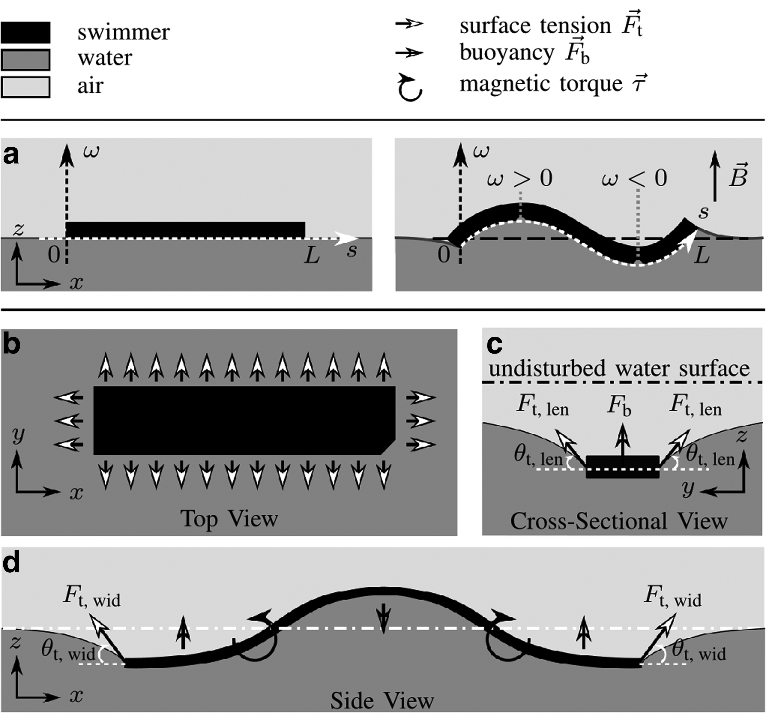
When a magnetic field is absent, a swimmer (length L, width W, and thickness T) at an air–water interface experiences gravity, buoyancy, and surface tension. At this state, the swimmer exhibits negligible deformation due to its low gravity and density values. Thus, it is assumed without much loss of accuracy that the swimmer has zero gravity, and it remains flat and does not disturb the air–water interface when no magnetic field is applied. Applying a magnetic field \documentclass{aastex}\usepackage{amsbsy}\usepackage{amsfonts}\usepackage{amssymb}\usepackage{bm}\usepackage{mathrsfs}\usepackage{pifont}\usepackage{stmaryrd}\usepackage{textcomp}\usepackage{portland, xspace}\usepackage{amsmath, amsxtra}\usepackage{upgreek}\pagestyle{empty}\DeclareMathSizes{10}{9}{7}{6}\begin{document}
$$\vec B$$
\end{document} causes a magnetic torque profile \documentclass{aastex}\usepackage{amsbsy}\usepackage{amsfonts}\usepackage{amssymb}\usepackage{bm}\usepackage{mathrsfs}\usepackage{pifont}\usepackage{stmaryrd}\usepackage{textcomp}\usepackage{portland, xspace}\usepackage{amsmath, amsxtra}\usepackage{upgreek}\pagestyle{empty}\DeclareMathSizes{10}{9}{7}{6}\begin{document}
$$\vec \tau \left( s \right)$$
\end{document} that is described by Eq. (2) and the swimmer deforms as a result. Since the swimmer rests on the air–water interface, its deformation interferes with the water surface and causes the surface tension \documentclass{aastex}\usepackage{amsbsy}\usepackage{amsfonts}\usepackage{amssymb}\usepackage{bm}\usepackage{mathrsfs}\usepackage{pifont}\usepackage{stmaryrd}\usepackage{textcomp}\usepackage{portland, xspace}\usepackage{amsmath, amsxtra}\usepackage{upgreek}\pagestyle{empty}\DeclareMathSizes{10}{9}{7}{6}\begin{document}
$${ \vec F_t}$$
\end{document} and the buoyancy \documentclass{aastex}\usepackage{amsbsy}\usepackage{amsfonts}\usepackage{amssymb}\usepackage{bm}\usepackage{mathrsfs}\usepackage{pifont}\usepackage{stmaryrd}\usepackage{textcomp}\usepackage{portland, xspace}\usepackage{amsmath, amsxtra}\usepackage{upgreek}\pagestyle{empty}\DeclareMathSizes{10}{9}{7}{6}\begin{document}
$${ \vec F_b}$$
\end{document} on it to change correspondingly. Moreover, the relative angle \documentclass{aastex}\usepackage{amsbsy}\usepackage{amsfonts}\usepackage{amssymb}\usepackage{bm}\usepackage{mathrsfs}\usepackage{pifont}\usepackage{stmaryrd}\usepackage{textcomp}\usepackage{portland, xspace}\usepackage{amsmath, amsxtra}\usepackage{upgreek}\pagestyle{empty}\DeclareMathSizes{10}{9}{7}{6}\begin{document}
$$\beta$$
\end{document} between \documentclass{aastex}\usepackage{amsbsy}\usepackage{amsfonts}\usepackage{amssymb}\usepackage{bm}\usepackage{mathrsfs}\usepackage{pifont}\usepackage{stmaryrd}\usepackage{textcomp}\usepackage{portland, xspace}\usepackage{amsmath, amsxtra}\usepackage{upgreek}\pagestyle{empty}\DeclareMathSizes{10}{9}{7}{6}\begin{document}
$$\vec M \left( s \right)$$
\end{document} and \documentclass{aastex}\usepackage{amsbsy}\usepackage{amsfonts}\usepackage{amssymb}\usepackage{bm}\usepackage{mathrsfs}\usepackage{pifont}\usepackage{stmaryrd}\usepackage{textcomp}\usepackage{portland, xspace}\usepackage{amsmath, amsxtra}\usepackage{upgreek}\pagestyle{empty}\DeclareMathSizes{10}{9}{7}{6}\begin{document}
$$\vec B$$
\end{document} changes as the swimmer deforms. Thus, the swimmer deformation converges to a shape that balances the internal shear forces and the external forces and torques.
As a convention, the positive direction of torques and forces are defined to be counterclockwise (from \documentclass{aastex}\usepackage{amsbsy}\usepackage{amsfonts}\usepackage{amssymb}\usepackage{bm}\usepackage{mathrsfs}\usepackage{pifont}\usepackage{stmaryrd}\usepackage{textcomp}\usepackage{portland, xspace}\usepackage{amsmath, amsxtra}\usepackage{upgreek}\pagestyle{empty}\DeclareMathSizes{10}{9}{7}{6}\begin{document}
$$+ x$$
\end{document} to \documentclass{aastex}\usepackage{amsbsy}\usepackage{amsfonts}\usepackage{amssymb}\usepackage{bm}\usepackage{mathrsfs}\usepackage{pifont}\usepackage{stmaryrd}\usepackage{textcomp}\usepackage{portland, xspace}\usepackage{amsmath, amsxtra}\usepackage{upgreek}\pagestyle{empty}\DeclareMathSizes{10}{9}{7}{6}\begin{document}
$$+ z$$
\end{document}) and upward (\documentclass{aastex}\usepackage{amsbsy}\usepackage{amsfonts}\usepackage{amssymb}\usepackage{bm}\usepackage{mathrsfs}\usepackage{pifont}\usepackage{stmaryrd}\usepackage{textcomp}\usepackage{portland, xspace}\usepackage{amsmath, amsxtra}\usepackage{upgreek}\pagestyle{empty}\DeclareMathSizes{10}{9}{7}{6}\begin{document}
$$ + z$$
\end{document}), respectively. The swimmer does not deform along its width, that is, axis y, and its shape is fully described by a shape profile \documentclass{aastex}\usepackage{amsbsy}\usepackage{amsfonts}\usepackage{amssymb}\usepackage{bm}\usepackage{mathrsfs}\usepackage{pifont}\usepackage{stmaryrd}\usepackage{textcomp}\usepackage{portland, xspace}\usepackage{amsmath, amsxtra}\usepackage{upgreek}\pagestyle{empty}\DeclareMathSizes{10}{9}{7}{6}\begin{document}
$$\omega \left( s \right)$$
\end{document} (\documentclass{aastex}\usepackage{amsbsy}\usepackage{amsfonts}\usepackage{amssymb}\usepackage{bm}\usepackage{mathrsfs}\usepackage{pifont}\usepackage{stmaryrd}\usepackage{textcomp}\usepackage{portland, xspace}\usepackage{amsmath, amsxtra}\usepackage{upgreek}\pagestyle{empty}\DeclareMathSizes{10}{9}{7}{6}\begin{document}
$$s \in$$
\end{document}[0, L]) in the x-z plane. The value of \documentclass{aastex}\usepackage{amsbsy}\usepackage{amsfonts}\usepackage{amssymb}\usepackage{bm}\usepackage{mathrsfs}\usepackage{pifont}\usepackage{stmaryrd}\usepackage{textcomp}\usepackage{portland, xspace}\usepackage{amsmath, amsxtra}\usepackage{upgreek}\pagestyle{empty}\DeclareMathSizes{10}{9}{7}{6}\begin{document}
$$\omega \left( s \right)$$
\end{document} is obtained by subtracting the height of the undisturbed water surface from the height of the swimmer bottom surface.
The forces and torques on the swimmer are schematically illustrated in Figure 4. Within the scenario discussed here, the swimmer deformation \documentclass{aastex}\usepackage{amsbsy}\usepackage{amsfonts}\usepackage{amssymb}\usepackage{bm}\usepackage{mathrsfs}\usepackage{pifont}\usepackage{stmaryrd}\usepackage{textcomp}\usepackage{portland, xspace}\usepackage{amsmath, amsxtra}\usepackage{upgreek}\pagestyle{empty}\DeclareMathSizes{10}{9}{7}{6}\begin{document}
$$\omega$$
\end{document} is always smaller than one tenth of its length L. Thus, the buoyancy \documentclass{aastex}\usepackage{amsbsy}\usepackage{amsfonts}\usepackage{amssymb}\usepackage{bm}\usepackage{mathrsfs}\usepackage{pifont}\usepackage{stmaryrd}\usepackage{textcomp}\usepackage{portland, xspace}\usepackage{amsmath, amsxtra}\usepackage{upgreek}\pagestyle{empty}\DeclareMathSizes{10}{9}{7}{6}\begin{document}
$${ \vec F_b}$$
\end{document} is considered to be always along axis z and its distribution \documentclass{aastex}\usepackage{amsbsy}\usepackage{amsfonts}\usepackage{amssymb}\usepackage{bm}\usepackage{mathrsfs}\usepackage{pifont}\usepackage{stmaryrd}\usepackage{textcomp}\usepackage{portland, xspace}\usepackage{amsmath, amsxtra}\usepackage{upgreek}\pagestyle{empty}\DeclareMathSizes{10}{9}{7}{6}\begin{document}
$${ \vec F_b} \left( s \right)$$
\end{document} with a unit of Newton per meter is calculated by
\documentclass{aastex}\usepackage{amsbsy}\usepackage{amsfonts}\usepackage{amssymb}\usepackage{bm}\usepackage{mathrsfs}\usepackage{pifont}\usepackage{stmaryrd}\usepackage{textcomp}\usepackage{portland, xspace}\usepackage{amsmath, amsxtra}\usepackage{upgreek}\pagestyle{empty}\DeclareMathSizes{10}{9}{7}{6}\begin{document}
\begin{align*}
{ \vec F_b} \left( s \right) = \rho gW \cdot \omega \left( s \right) \tag{3} ,
\end{align*}
\end{document}
On-water swimmer shape definition and the forces and torques it experiences. The swimmer shape is described by \documentclass{aastex}\usepackage{amsbsy}\usepackage{amsfonts}\usepackage{amssymb}\usepackage{bm}\usepackage{mathrsfs}\usepackage{pifont}\usepackage{stmaryrd}\usepackage{textcomp}\usepackage{portland, xspace}\usepackage{amsmath, amsxtra}\usepackage{upgreek}\pagestyle{empty}\DeclareMathSizes{10}{9}{7}{6}\begin{document}
$$\omega$$
\end{document} and defined in (a). The swimmer deforms when a magnetic field is applied and interacts with the water surface. The forces and torques applied on the swimmer when it deforms are qualitatively drawn in the top view, cross-sectional view, and side view in (b–d), respectively. The surface tension applied along the swimmer length is not shown in (d) for better visibility. The arrow sizes do not represent the corresponding force magnitudes.
where \documentclass{aastex}\usepackage{amsbsy}\usepackage{amsfonts}\usepackage{amssymb}\usepackage{bm}\usepackage{mathrsfs}\usepackage{pifont}\usepackage{stmaryrd}\usepackage{textcomp}\usepackage{portland, xspace}\usepackage{amsmath, amsxtra}\usepackage{upgreek}\pagestyle{empty}\DeclareMathSizes{10}{9}{7}{6}\begin{document}
$$\rho$$
\end{document} is the water density (1000 kg/\documentclass{aastex}\usepackage{amsbsy}\usepackage{amsfonts}\usepackage{amssymb}\usepackage{bm}\usepackage{mathrsfs}\usepackage{pifont}\usepackage{stmaryrd}\usepackage{textcomp}\usepackage{portland, xspace}\usepackage{amsmath, amsxtra}\usepackage{upgreek}\pagestyle{empty}\DeclareMathSizes{10}{9}{7}{6}\begin{document}
$${{ \rm{m}}^3}$$
\end{document}), g is the gravitational acceleration constant (9.8 m/\documentclass{aastex}\usepackage{amsbsy}\usepackage{amsfonts}\usepackage{amssymb}\usepackage{bm}\usepackage{mathrsfs}\usepackage{pifont}\usepackage{stmaryrd}\usepackage{textcomp}\usepackage{portland, xspace}\usepackage{amsmath, amsxtra}\usepackage{upgreek}\pagestyle{empty}\DeclareMathSizes{10}{9}{7}{6}\begin{document}
$${{ \rm{s}}^2}$$
\end{document}), and W is the swimmer width in meter. The surface tension \documentclass{aastex}\usepackage{amsbsy}\usepackage{amsfonts}\usepackage{amssymb}\usepackage{bm}\usepackage{mathrsfs}\usepackage{pifont}\usepackage{stmaryrd}\usepackage{textcomp}\usepackage{portland, xspace}\usepackage{amsmath, amsxtra}\usepackage{upgreek}\pagestyle{empty}\DeclareMathSizes{10}{9}{7}{6}\begin{document}
$${ \vec F_t}$$
\end{document} exists at the boundary of the contact area between the swimmer and the water. The direction of \documentclass{aastex}\usepackage{amsbsy}\usepackage{amsfonts}\usepackage{amssymb}\usepackage{bm}\usepackage{mathrsfs}\usepackage{pifont}\usepackage{stmaryrd}\usepackage{textcomp}\usepackage{portland, xspace}\usepackage{amsmath, amsxtra}\usepackage{upgreek}\pagestyle{empty}\DeclareMathSizes{10}{9}{7}{6}\begin{document}
$${ \vec F_t}$$
\end{document} is along the disturbed water surface and perpendicular to the boundary, forming an angle \documentclass{aastex}\usepackage{amsbsy}\usepackage{amsfonts}\usepackage{amssymb}\usepackage{bm}\usepackage{mathrsfs}\usepackage{pifont}\usepackage{stmaryrd}\usepackage{textcomp}\usepackage{portland, xspace}\usepackage{amsmath, amsxtra}\usepackage{upgreek}\pagestyle{empty}\DeclareMathSizes{10}{9}{7}{6}\begin{document}
$${ \theta _t}$$
\end{document} with the horizontal plane. The \documentclass{aastex}\usepackage{amsbsy}\usepackage{amsfonts}\usepackage{amssymb}\usepackage{bm}\usepackage{mathrsfs}\usepackage{pifont}\usepackage{stmaryrd}\usepackage{textcomp}\usepackage{portland, xspace}\usepackage{amsmath, amsxtra}\usepackage{upgreek}\pagestyle{empty}\DeclareMathSizes{10}{9}{7}{6}\begin{document}
$${ \vec F_t}$$
\end{document} along the swimmer length and width are denoted by \documentclass{aastex}\usepackage{amsbsy}\usepackage{amsfonts}\usepackage{amssymb}\usepackage{bm}\usepackage{mathrsfs}\usepackage{pifont}\usepackage{stmaryrd}\usepackage{textcomp}\usepackage{portland, xspace}\usepackage{amsmath, amsxtra}\usepackage{upgreek}\pagestyle{empty}\DeclareMathSizes{10}{9}{7}{6}\begin{document}
$${ \vec F_{{ \rm{t , \;len}}}}$$
\end{document} and \documentclass{aastex}\usepackage{amsbsy}\usepackage{amsfonts}\usepackage{amssymb}\usepackage{bm}\usepackage{mathrsfs}\usepackage{pifont}\usepackage{stmaryrd}\usepackage{textcomp}\usepackage{portland, xspace}\usepackage{amsmath, amsxtra}\usepackage{upgreek}\pagestyle{empty}\DeclareMathSizes{10}{9}{7}{6}\begin{document}
$${ \vec F_{{ \rm{t , \;wid}}}}$$
\end{document}, respectively. The horizontal component of \documentclass{aastex}\usepackage{amsbsy}\usepackage{amsfonts}\usepackage{amssymb}\usepackage{bm}\usepackage{mathrsfs}\usepackage{pifont}\usepackage{stmaryrd}\usepackage{textcomp}\usepackage{portland, xspace}\usepackage{amsmath, amsxtra}\usepackage{upgreek}\pagestyle{empty}\DeclareMathSizes{10}{9}{7}{6}\begin{document}
$${ \vec F_{{ \rm{t , \;len}}}}$$
\end{document} points along axis y and does not affect the swimmer shape \documentclass{aastex}\usepackage{amsbsy}\usepackage{amsfonts}\usepackage{amssymb}\usepackage{bm}\usepackage{mathrsfs}\usepackage{pifont}\usepackage{stmaryrd}\usepackage{textcomp}\usepackage{portland, xspace}\usepackage{amsmath, amsxtra}\usepackage{upgreek}\pagestyle{empty}\DeclareMathSizes{10}{9}{7}{6}\begin{document}
$$\omega$$
\end{document} in the x-z plane. The vertical component of \documentclass{aastex}\usepackage{amsbsy}\usepackage{amsfonts}\usepackage{amssymb}\usepackage{bm}\usepackage{mathrsfs}\usepackage{pifont}\usepackage{stmaryrd}\usepackage{textcomp}\usepackage{portland, xspace}\usepackage{amsmath, amsxtra}\usepackage{upgreek}\pagestyle{empty}\DeclareMathSizes{10}{9}{7}{6}\begin{document}
$${ \vec F_{{ \rm{t , \;len}}}}$$
\end{document}, that is, \documentclass{aastex}\usepackage{amsbsy}\usepackage{amsfonts}\usepackage{amssymb}\usepackage{bm}\usepackage{mathrsfs}\usepackage{pifont}\usepackage{stmaryrd}\usepackage{textcomp}\usepackage{portland, xspace}\usepackage{amsmath, amsxtra}\usepackage{upgreek}\pagestyle{empty}\DeclareMathSizes{10}{9}{7}{6}\begin{document}
$${ \vec F_{{ \rm{t , \;len , \;v}}}}$$
\end{document}, and \documentclass{aastex}\usepackage{amsbsy}\usepackage{amsfonts}\usepackage{amssymb}\usepackage{bm}\usepackage{mathrsfs}\usepackage{pifont}\usepackage{stmaryrd}\usepackage{textcomp}\usepackage{portland, xspace}\usepackage{amsmath, amsxtra}\usepackage{upgreek}\pagestyle{empty}\DeclareMathSizes{10}{9}{7}{6}\begin{document}
$${ \vec F_{{ \rm{t , \;wid}}}}$$
\end{document} are relevant with \documentclass{aastex}\usepackage{amsbsy}\usepackage{amsfonts}\usepackage{amssymb}\usepackage{bm}\usepackage{mathrsfs}\usepackage{pifont}\usepackage{stmaryrd}\usepackage{textcomp}\usepackage{portland, xspace}\usepackage{amsmath, amsxtra}\usepackage{upgreek}\pagestyle{empty}\DeclareMathSizes{10}{9}{7}{6}\begin{document}
$$\omega$$
\end{document} and computed correspondingly as
\documentclass{aastex}\usepackage{amsbsy}\usepackage{amsfonts}\usepackage{amssymb}\usepackage{bm}\usepackage{mathrsfs}\usepackage{pifont}\usepackage{stmaryrd}\usepackage{textcomp}\usepackage{portland, xspace}\usepackage{amsmath, amsxtra}\usepackage{upgreek}\pagestyle{empty}\DeclareMathSizes{10}{9}{7}{6}\begin{document}
\begin{align*}
{ \left. {{F_{{ \rm{t , \;len , \;v}}}} \left( s \right) } \right\vert _{s \in \left[ {0 , \;L} \right] }} = 2 \gamma \sin { \theta _t} \left( s \right) \tag{4}
\end{align*}
\end{document}\documentclass{aastex}\usepackage{amsbsy}\usepackage{amsfonts}\usepackage{amssymb}\usepackage{bm}\usepackage{mathrsfs}\usepackage{pifont}\usepackage{stmaryrd}\usepackage{textcomp}\usepackage{portland, xspace}\usepackage{amsmath, amsxtra}\usepackage{upgreek}\pagestyle{empty}\DeclareMathSizes{10}{9}{7}{6}\begin{document}
\begin{align*}
{ \left. {{F_{{ \rm{t , \;wid , \;v}}}} \left( s \right) } \right\vert _{s \in \left[ {0 , \;L} \right] }} = \gamma W \sin { \theta _t} \left( s \right) \tag{5}
\end{align*}
\end{document}
and
\documentclass{aastex}\usepackage{amsbsy}\usepackage{amsfonts}\usepackage{amssymb}\usepackage{bm}\usepackage{mathrsfs}\usepackage{pifont}\usepackage{stmaryrd}\usepackage{textcomp}\usepackage{portland, xspace}\usepackage{amsmath, amsxtra}\usepackage{upgreek}\pagestyle{empty}\DeclareMathSizes{10}{9}{7}{6}\begin{document}
\begin{align*}
{ \left. {{F_{{ \rm{t , \;wid , \;h}}}} \left( s \right) } \right\vert _{s \in \left[ {0 , \;L} \right] }} = \gamma W \cos { \theta _t} \left( s \right) \tag{6} ,
\end{align*}
\end{document}
respectively. The constant \documentclass{aastex}\usepackage{amsbsy}\usepackage{amsfonts}\usepackage{amssymb}\usepackage{bm}\usepackage{mathrsfs}\usepackage{pifont}\usepackage{stmaryrd}\usepackage{textcomp}\usepackage{portland, xspace}\usepackage{amsmath, amsxtra}\usepackage{upgreek}\pagestyle{empty}\DeclareMathSizes{10}{9}{7}{6}\begin{document}
$$\gamma$$
\end{document} is the surface tension coefficient (0.072 N/m for an air–water interface). The force profile \documentclass{aastex}\usepackage{amsbsy}\usepackage{amsfonts}\usepackage{amssymb}\usepackage{bm}\usepackage{mathrsfs}\usepackage{pifont}\usepackage{stmaryrd}\usepackage{textcomp}\usepackage{portland, xspace}\usepackage{amsmath, amsxtra}\usepackage{upgreek}\pagestyle{empty}\DeclareMathSizes{10}{9}{7}{6}\begin{document}
$${F_{{ \rm{t , \;len , \;v}}}} \left( s \right)$$
\end{document} has a coefficient of 2 because both long edges of the swimmer experience the surface tension forces with the same vertical components. Note that \documentclass{aastex}\usepackage{amsbsy}\usepackage{amsfonts}\usepackage{amssymb}\usepackage{bm}\usepackage{mathrsfs}\usepackage{pifont}\usepackage{stmaryrd}\usepackage{textcomp}\usepackage{portland, xspace}\usepackage{amsmath, amsxtra}\usepackage{upgreek}\pagestyle{empty}\DeclareMathSizes{10}{9}{7}{6}\begin{document}
$${F_{{ \rm{t , \;len , \;v}}}} \left( s \right)$$
\end{document} has a unit of Newton per meter, whereas \documentclass{aastex}\usepackage{amsbsy}\usepackage{amsfonts}\usepackage{amssymb}\usepackage{bm}\usepackage{mathrsfs}\usepackage{pifont}\usepackage{stmaryrd}\usepackage{textcomp}\usepackage{portland, xspace}\usepackage{amsmath, amsxtra}\usepackage{upgreek}\pagestyle{empty}\DeclareMathSizes{10}{9}{7}{6}\begin{document}
$${F_{{ \rm{t , \;wid , \;v}}}} \left( s \right)$$
\end{document} and \documentclass{aastex}\usepackage{amsbsy}\usepackage{amsfonts}\usepackage{amssymb}\usepackage{bm}\usepackage{mathrsfs}\usepackage{pifont}\usepackage{stmaryrd}\usepackage{textcomp}\usepackage{portland, xspace}\usepackage{amsmath, amsxtra}\usepackage{upgreek}\pagestyle{empty}\DeclareMathSizes{10}{9}{7}{6}\begin{document}
$${F_{{ \rm{t , \;wid , \;h}}}} \left( s \right)$$
\end{document} have a unit of Newton. This difference is because \documentclass{aastex}\usepackage{amsbsy}\usepackage{amsfonts}\usepackage{amssymb}\usepackage{bm}\usepackage{mathrsfs}\usepackage{pifont}\usepackage{stmaryrd}\usepackage{textcomp}\usepackage{portland, xspace}\usepackage{amsmath, amsxtra}\usepackage{upgreek}\pagestyle{empty}\DeclareMathSizes{10}{9}{7}{6}\begin{document}
$${F_{{ \rm{t , \;len , \;v}}}} \left( s \right)$$
\end{document} is a force profile, but \documentclass{aastex}\usepackage{amsbsy}\usepackage{amsfonts}\usepackage{amssymb}\usepackage{bm}\usepackage{mathrsfs}\usepackage{pifont}\usepackage{stmaryrd}\usepackage{textcomp}\usepackage{portland, xspace}\usepackage{amsmath, amsxtra}\usepackage{upgreek}\pagestyle{empty}\DeclareMathSizes{10}{9}{7}{6}\begin{document}
$${F_{{ \rm{t , \;wid , \;v}}}} \left( s \right)$$
\end{document} and \documentclass{aastex}\usepackage{amsbsy}\usepackage{amsfonts}\usepackage{amssymb}\usepackage{bm}\usepackage{mathrsfs}\usepackage{pifont}\usepackage{stmaryrd}\usepackage{textcomp}\usepackage{portland, xspace}\usepackage{amsmath, amsxtra}\usepackage{upgreek}\pagestyle{empty}\DeclareMathSizes{10}{9}{7}{6}\begin{document}
$${F_{{ \rm{t , \;wid , \;h}}}} \left( s \right)$$
\end{document} are force components.
The total bending moment \documentclass{aastex}\usepackage{amsbsy}\usepackage{amsfonts}\usepackage{amssymb}\usepackage{bm}\usepackage{mathrsfs}\usepackage{pifont}\usepackage{stmaryrd}\usepackage{textcomp}\usepackage{portland, xspace}\usepackage{amsmath, amsxtra}\usepackage{upgreek}\pagestyle{empty}\DeclareMathSizes{10}{9}{7}{6}\begin{document}
$$Q \left( s \right)$$
\end{document} on the swimmer body is
\documentclass{aastex}\usepackage{amsbsy}\usepackage{amsfonts}\usepackage{amssymb}\usepackage{bm}\usepackage{mathrsfs}\usepackage{pifont}\usepackage{stmaryrd}\usepackage{textcomp}\usepackage{portland, xspace}\usepackage{amsmath, amsxtra}\usepackage{upgreek}\pagestyle{empty}\DeclareMathSizes{10}{9}{7}{6}\begin{document}
\begin{align*}
Q \left( s \right) = {Q_ \tau } \left( s \right) + {Q_b} \left( s \right) + {Q_t} \left( s \right) \tag{7} ,
\end{align*}
\end{document}
where \documentclass{aastex}\usepackage{amsbsy}\usepackage{amsfonts}\usepackage{amssymb}\usepackage{bm}\usepackage{mathrsfs}\usepackage{pifont}\usepackage{stmaryrd}\usepackage{textcomp}\usepackage{portland, xspace}\usepackage{amsmath, amsxtra}\usepackage{upgreek}\pagestyle{empty}\DeclareMathSizes{10}{9}{7}{6}\begin{document}
$${Q_ \tau } \left( s \right)$$
\end{document}, \documentclass{aastex}\usepackage{amsbsy}\usepackage{amsfonts}\usepackage{amssymb}\usepackage{bm}\usepackage{mathrsfs}\usepackage{pifont}\usepackage{stmaryrd}\usepackage{textcomp}\usepackage{portland, xspace}\usepackage{amsmath, amsxtra}\usepackage{upgreek}\pagestyle{empty}\DeclareMathSizes{10}{9}{7}{6}\begin{document}
$${Q_t} \left( s \right)$$
\end{document}, and \documentclass{aastex}\usepackage{amsbsy}\usepackage{amsfonts}\usepackage{amssymb}\usepackage{bm}\usepackage{mathrsfs}\usepackage{pifont}\usepackage{stmaryrd}\usepackage{textcomp}\usepackage{portland, xspace}\usepackage{amsmath, amsxtra}\usepackage{upgreek}\pagestyle{empty}\DeclareMathSizes{10}{9}{7}{6}\begin{document}
$${Q_b} \left( s \right)$$
\end{document} are the bending moment caused by the magnetic torque \documentclass{aastex}\usepackage{amsbsy}\usepackage{amsfonts}\usepackage{amssymb}\usepackage{bm}\usepackage{mathrsfs}\usepackage{pifont}\usepackage{stmaryrd}\usepackage{textcomp}\usepackage{portland, xspace}\usepackage{amsmath, amsxtra}\usepackage{upgreek}\pagestyle{empty}\DeclareMathSizes{10}{9}{7}{6}\begin{document}
$$\vec \tau$$
\end{document}, surface tension \documentclass{aastex}\usepackage{amsbsy}\usepackage{amsfonts}\usepackage{amssymb}\usepackage{bm}\usepackage{mathrsfs}\usepackage{pifont}\usepackage{stmaryrd}\usepackage{textcomp}\usepackage{portland, xspace}\usepackage{amsmath, amsxtra}\usepackage{upgreek}\pagestyle{empty}\DeclareMathSizes{10}{9}{7}{6}\begin{document}
$${ \vec F_t}$$
\end{document}, and buoyancy \documentclass{aastex}\usepackage{amsbsy}\usepackage{amsfonts}\usepackage{amssymb}\usepackage{bm}\usepackage{mathrsfs}\usepackage{pifont}\usepackage{stmaryrd}\usepackage{textcomp}\usepackage{portland, xspace}\usepackage{amsmath, amsxtra}\usepackage{upgreek}\pagestyle{empty}\DeclareMathSizes{10}{9}{7}{6}\begin{document}
$${ \vec F_b}$$
\end{document}, respectively, and they can be calculated using the relationship between the load, shear force, and bending moment on a beam. The bending moment \documentclass{aastex}\usepackage{amsbsy}\usepackage{amsfonts}\usepackage{amssymb}\usepackage{bm}\usepackage{mathrsfs}\usepackage{pifont}\usepackage{stmaryrd}\usepackage{textcomp}\usepackage{portland, xspace}\usepackage{amsmath, amsxtra}\usepackage{upgreek}\pagestyle{empty}\DeclareMathSizes{10}{9}{7}{6}\begin{document}
$${Q_ \tau }$$
\end{document} and Qb are computed as
\documentclass{aastex}\usepackage{amsbsy}\usepackage{amsfonts}\usepackage{amssymb}\usepackage{bm}\usepackage{mathrsfs}\usepackage{pifont}\usepackage{stmaryrd}\usepackage{textcomp}\usepackage{portland, xspace}\usepackage{amsmath, amsxtra}\usepackage{upgreek}\pagestyle{empty}\DeclareMathSizes{10}{9}{7}{6}\begin{document}
\begin{align*}
{Q_ \tau } \left( s \right) = - \int_0^s { \tau \left( { \tilde s} \right) { \rm{d}} \tilde s} \tag{8}
\end{align*}
\end{document}
respectively. The dummy variable \documentclass{aastex}\usepackage{amsbsy}\usepackage{amsfonts}\usepackage{amssymb}\usepackage{bm}\usepackage{mathrsfs}\usepackage{pifont}\usepackage{stmaryrd}\usepackage{textcomp}\usepackage{portland, xspace}\usepackage{amsmath, amsxtra}\usepackage{upgreek}\pagestyle{empty}\DeclareMathSizes{10}{9}{7}{6}\begin{document}
$$\tilde S$$
\end{document} is a placeholder and disappears completely in final results. The bending moment Qt is further divided into
\documentclass{aastex}\usepackage{amsbsy}\usepackage{amsfonts}\usepackage{amssymb}\usepackage{bm}\usepackage{mathrsfs}\usepackage{pifont}\usepackage{stmaryrd}\usepackage{textcomp}\usepackage{portland, xspace}\usepackage{amsmath, amsxtra}\usepackage{upgreek}\pagestyle{empty}\DeclareMathSizes{10}{9}{7}{6}\begin{document}
\begin{align*}
{Q_t} \left( s \right) = {Q_{{ \rm{t , \;len , \;v}}}} \left( s \right) + {Q_{{ \rm{t , \;wid , \;v}}}} \left( s \right) + {Q_{{ \rm{t , \;wid , \;h}}}} \left( s \right) \tag{10} ,
\end{align*}
\end{document}
As mentioned before, the swimmer deformation \documentclass{aastex}\usepackage{amsbsy}\usepackage{amsfonts}\usepackage{amssymb}\usepackage{bm}\usepackage{mathrsfs}\usepackage{pifont}\usepackage{stmaryrd}\usepackage{textcomp}\usepackage{portland, xspace}\usepackage{amsmath, amsxtra}\usepackage{upgreek}\pagestyle{empty}\DeclareMathSizes{10}{9}{7}{6}\begin{document}
$$\omega$$
\end{document} is always smaller than one tenth of its length L, satisfying the “small deformation” assumption of the Euler–Bernoulli beam theory. Thus, the curvature \documentclass{aastex}\usepackage{amsbsy}\usepackage{amsfonts}\usepackage{amssymb}\usepackage{bm}\usepackage{mathrsfs}\usepackage{pifont}\usepackage{stmaryrd}\usepackage{textcomp}\usepackage{portland, xspace}\usepackage{amsmath, amsxtra}\usepackage{upgreek}\pagestyle{empty}\DeclareMathSizes{10}{9}{7}{6}\begin{document}
$$\kappa$$
\end{document} of the swimmer body is related to its bending moment Q using the Euler–Bernoulli beam theory as
\documentclass{aastex}\usepackage{amsbsy}\usepackage{amsfonts}\usepackage{amssymb}\usepackage{bm}\usepackage{mathrsfs}\usepackage{pifont}\usepackage{stmaryrd}\usepackage{textcomp}\usepackage{portland, xspace}\usepackage{amsmath, amsxtra}\usepackage{upgreek}\pagestyle{empty}\DeclareMathSizes{10}{9}{7}{6}\begin{document}
\begin{align*}
\kappa \left( s \right) = Q \left( s \right) \cdot { \left( {EI} \right) ^{ - 1}} \tag{14}
\end{align*}
\end{document}
where E and \documentclass{aastex}\usepackage{amsbsy}\usepackage{amsfonts}\usepackage{amssymb}\usepackage{bm}\usepackage{mathrsfs}\usepackage{pifont}\usepackage{stmaryrd}\usepackage{textcomp}\usepackage{portland, xspace}\usepackage{amsmath, amsxtra}\usepackage{upgreek}\pagestyle{empty}\DeclareMathSizes{10}{9}{7}{6}\begin{document}
$$I = W{T^3} / 12$$
\end{document} are the Young's modulus and the second moment of area of the swimmer sheet, respectively. Finally, the swimmer shape profile \documentclass{aastex}\usepackage{amsbsy}\usepackage{amsfonts}\usepackage{amssymb}\usepackage{bm}\usepackage{mathrsfs}\usepackage{pifont}\usepackage{stmaryrd}\usepackage{textcomp}\usepackage{portland, xspace}\usepackage{amsmath, amsxtra}\usepackage{upgreek}\pagestyle{empty}\DeclareMathSizes{10}{9}{7}{6}\begin{document}
$$\omega \left( s \right)$$
\end{document} can be derived from its curvature profile \documentclass{aastex}\usepackage{amsbsy}\usepackage{amsfonts}\usepackage{amssymb}\usepackage{bm}\usepackage{mathrsfs}\usepackage{pifont}\usepackage{stmaryrd}\usepackage{textcomp}\usepackage{portland, xspace}\usepackage{amsmath, amsxtra}\usepackage{upgreek}\pagestyle{empty}\DeclareMathSizes{10}{9}{7}{6}\begin{document}
$$\kappa \left( s \right)$$
\end{document}.
Parameter measurement
The parameters relevant to the proposed swimmer shape model were measured independently, to theoretically predict the swimmer shapes from underlying physical principles and verify the model efficacy by comparing predictions against observations. This specific swimmer had dimensional values of 4.47\documentclass{aastex}\usepackage{amsbsy}\usepackage{amsfonts}\usepackage{amssymb}\usepackage{bm}\usepackage{mathrsfs}\usepackage{pifont}\usepackage{stmaryrd}\usepackage{textcomp}\usepackage{portland, xspace}\usepackage{amsmath, amsxtra}\usepackage{upgreek}\pagestyle{empty}\DeclareMathSizes{10}{9}{7}{6}\begin{document}
$$\times$$
\end{document}1.33\documentclass{aastex}\usepackage{amsbsy}\usepackage{amsfonts}\usepackage{amssymb}\usepackage{bm}\usepackage{mathrsfs}\usepackage{pifont}\usepackage{stmaryrd}\usepackage{textcomp}\usepackage{portland, xspace}\usepackage{amsmath, amsxtra}\usepackage{upgreek}\pagestyle{empty}\DeclareMathSizes{10}{9}{7}{6}\begin{document}
$$\times$$
\end{document}0.109 \documentclass{aastex}\usepackage{amsbsy}\usepackage{amsfonts}\usepackage{amssymb}\usepackage{bm}\usepackage{mathrsfs}\usepackage{pifont}\usepackage{stmaryrd}\usepackage{textcomp}\usepackage{portland, xspace}\usepackage{amsmath, amsxtra}\usepackage{upgreek}\pagestyle{empty}\DeclareMathSizes{10}{9}{7}{6}\begin{document}
$${ \rm{m}}{{ \rm{m}}^3}$$
\end{document} (length, width, and thickness). The length and width were measured using a caliper (Starrett, resolution 0.01 mm) and the thickness was measured by a micrometer (Mitutoyo, resolution 0.001 mm). The applied magnetic field in the shape observation experiment had a strength of 10 mT, which was verified by a gaussmeter (Model 425, LakeShore).
The swimmer magnetization could not be measured directly because its direction varied along the body. Thus, eight cubes with a side length of 3.1 mm were made of the soft magnetic composite that was used by the swimmer. These cubes were magnetized in the same magnetizing setup with the swimmer, and then glued into a larger cube that exhibits a stronger overall magnetic moment. The magnetic field of the larger cube was measured using the gaussmeter at several known distances from the cube. The obtained data were fitted to a magnetic dipole model to estimate the magnetic moment. A magnetization value was obtained by dividing the magnetic moment by the total volume of the cube. The obtained magnetization value of the cube was assumed to be identical with the swimmer magnetization, because they shared the same material and went through the same magnetizing process. The magnitude of magnetization of the soft magnetic composite was measured to be 45 kA/m.
Another parameter that needed to be measured is the Young's modulus E of the sheet. In the measurement, a sheet was fixed by one end and leaving the other one free. A microforce sensing probe (FT-S100 probe, FemtoTools) applied a point force on the sheet to bend it, mimicking the sheet deformation when it swims. This experiment is illustrated in Supplementary Figure S3. The value of \documentclass{aastex}\usepackage{amsbsy}\usepackage{amsfonts}\usepackage{amssymb}\usepackage{bm}\usepackage{mathrsfs}\usepackage{pifont}\usepackage{stmaryrd}\usepackage{textcomp}\usepackage{portland, xspace}\usepackage{amsmath, amsxtra}\usepackage{upgreek}\pagestyle{empty}\DeclareMathSizes{10}{9}{7}{6}\begin{document}
$$E = 0.165$$
\end{document} MPa was derived from the recorded values of the force amplitude and corresponding deformation. Detailed results of this measurement can be found in Supplementary Table S1.
Numerical simulation of swimmer shapes
With the proposed shape model and the measured parameter values, there is only one problem left to be addressed before the swimmer shape can be simulated from first principles: The swimmer has sharp edges, whose interaction with the water surface is complex and hinders the analysis of the surface tension \documentclass{aastex}\usepackage{amsbsy}\usepackage{amsfonts}\usepackage{amssymb}\usepackage{bm}\usepackage{mathrsfs}\usepackage{pifont}\usepackage{stmaryrd}\usepackage{textcomp}\usepackage{portland, xspace}\usepackage{amsmath, amsxtra}\usepackage{upgreek}\pagestyle{empty}\DeclareMathSizes{10}{9}{7}{6}\begin{document}
$${ \vec F_t}$$
\end{document} (Fig. 5a). A vertical swimmer edge is described as a combination of a straight line segment and two quadrants (radius \documentclass{aastex}\usepackage{amsbsy}\usepackage{amsfonts}\usepackage{amssymb}\usepackage{bm}\usepackage{mathrsfs}\usepackage{pifont}\usepackage{stmaryrd}\usepackage{textcomp}\usepackage{portland, xspace}\usepackage{amsmath, amsxtra}\usepackage{upgreek}\pagestyle{empty}\DeclareMathSizes{10}{9}{7}{6}\begin{document}
$$r \ge 0$$
\end{document}) at both ends. When the water–air–swimmer (WAS) intersection is within the quadrant region, the surface tension angle \documentclass{aastex}\usepackage{amsbsy}\usepackage{amsfonts}\usepackage{amssymb}\usepackage{bm}\usepackage{mathrsfs}\usepackage{pifont}\usepackage{stmaryrd}\usepackage{textcomp}\usepackage{portland, xspace}\usepackage{amsmath, amsxtra}\usepackage{upgreek}\pagestyle{empty}\DeclareMathSizes{10}{9}{7}{6}\begin{document}
$${ \theta _t}$$
\end{document} is related to the contact angle \documentclass{aastex}\usepackage{amsbsy}\usepackage{amsfonts}\usepackage{amssymb}\usepackage{bm}\usepackage{mathrsfs}\usepackage{pifont}\usepackage{stmaryrd}\usepackage{textcomp}\usepackage{portland, xspace}\usepackage{amsmath, amsxtra}\usepackage{upgreek}\pagestyle{empty}\DeclareMathSizes{10}{9}{7}{6}\begin{document}
$${ \theta _c}$$
\end{document} and the submerge angle \documentclass{aastex}\usepackage{amsbsy}\usepackage{amsfonts}\usepackage{amssymb}\usepackage{bm}\usepackage{mathrsfs}\usepackage{pifont}\usepackage{stmaryrd}\usepackage{textcomp}\usepackage{portland, xspace}\usepackage{amsmath, amsxtra}\usepackage{upgreek}\pagestyle{empty}\DeclareMathSizes{10}{9}{7}{6}\begin{document}
$$\delta$$
\end{document} as \documentclass{aastex}\usepackage{amsbsy}\usepackage{amsfonts}\usepackage{amssymb}\usepackage{bm}\usepackage{mathrsfs}\usepackage{pifont}\usepackage{stmaryrd}\usepackage{textcomp}\usepackage{portland, xspace}\usepackage{amsmath, amsxtra}\usepackage{upgreek}\pagestyle{empty}\DeclareMathSizes{10}{9}{7}{6}\begin{document}
$${ \theta _t} = { \theta _c} + \delta - \pi$$
\end{document}. The value of \documentclass{aastex}\usepackage{amsbsy}\usepackage{amsfonts}\usepackage{amssymb}\usepackage{bm}\usepackage{mathrsfs}\usepackage{pifont}\usepackage{stmaryrd}\usepackage{textcomp}\usepackage{portland, xspace}\usepackage{amsmath, amsxtra}\usepackage{upgreek}\pagestyle{empty}\DeclareMathSizes{10}{9}{7}{6}\begin{document}
$${ \theta _t}$$
\end{document} increases with \documentclass{aastex}\usepackage{amsbsy}\usepackage{amsfonts}\usepackage{amssymb}\usepackage{bm}\usepackage{mathrsfs}\usepackage{pifont}\usepackage{stmaryrd}\usepackage{textcomp}\usepackage{portland, xspace}\usepackage{amsmath, amsxtra}\usepackage{upgreek}\pagestyle{empty}\DeclareMathSizes{10}{9}{7}{6}\begin{document}
$$\delta$$
\end{document} as the swimmer goes further down into the water until the WAS intersection moves into the line segment region, where \documentclass{aastex}\usepackage{amsbsy}\usepackage{amsfonts}\usepackage{amssymb}\usepackage{bm}\usepackage{mathrsfs}\usepackage{pifont}\usepackage{stmaryrd}\usepackage{textcomp}\usepackage{portland, xspace}\usepackage{amsmath, amsxtra}\usepackage{upgreek}\pagestyle{empty}\DeclareMathSizes{10}{9}{7}{6}\begin{document}
$${ \theta _t}$$
\end{document} is constant and \documentclass{aastex}\usepackage{amsbsy}\usepackage{amsfonts}\usepackage{amssymb}\usepackage{bm}\usepackage{mathrsfs}\usepackage{pifont}\usepackage{stmaryrd}\usepackage{textcomp}\usepackage{portland, xspace}\usepackage{amsmath, amsxtra}\usepackage{upgreek}\pagestyle{empty}\DeclareMathSizes{10}{9}{7}{6}\begin{document}
$${ \theta _t} = { \theta _c} - \pi / 2$$
\end{document}. Since the swimmer thickness T is small compared with its other dimensions and deformation magnitude, the thickness T is neglected in the calculation of the swimmer shape \documentclass{aastex}\usepackage{amsbsy}\usepackage{amsfonts}\usepackage{amssymb}\usepackage{bm}\usepackage{mathrsfs}\usepackage{pifont}\usepackage{stmaryrd}\usepackage{textcomp}\usepackage{portland, xspace}\usepackage{amsmath, amsxtra}\usepackage{upgreek}\pagestyle{empty}\DeclareMathSizes{10}{9}{7}{6}\begin{document}
$$\omega$$
\end{document} and the swimmer edge is approximated as a hemisphere with infinitesimal radius, that is, \documentclass{aastex}\usepackage{amsbsy}\usepackage{amsfonts}\usepackage{amssymb}\usepackage{bm}\usepackage{mathrsfs}\usepackage{pifont}\usepackage{stmaryrd}\usepackage{textcomp}\usepackage{portland, xspace}\usepackage{amsmath, amsxtra}\usepackage{upgreek}\pagestyle{empty}\DeclareMathSizes{10}{9}{7}{6}\begin{document}
$$r \to 0$$
\end{document}. As a result, the value of \documentclass{aastex}\usepackage{amsbsy}\usepackage{amsfonts}\usepackage{amssymb}\usepackage{bm}\usepackage{mathrsfs}\usepackage{pifont}\usepackage{stmaryrd}\usepackage{textcomp}\usepackage{portland, xspace}\usepackage{amsmath, amsxtra}\usepackage{upgreek}\pagestyle{empty}\DeclareMathSizes{10}{9}{7}{6}\begin{document}
$${ \theta _t}$$
\end{document} varies with \documentclass{aastex}\usepackage{amsbsy}\usepackage{amsfonts}\usepackage{amssymb}\usepackage{bm}\usepackage{mathrsfs}\usepackage{pifont}\usepackage{stmaryrd}\usepackage{textcomp}\usepackage{portland, xspace}\usepackage{amsmath, amsxtra}\usepackage{upgreek}\pagestyle{empty}\DeclareMathSizes{10}{9}{7}{6}\begin{document}
$$\omega$$
\end{document}, whereas the WAS intersection remains at the same spot on the swimmer.
The sharp edge problem of the swimmer and its treatment. A sharp swimmer edge is represented by the combination of a line segment and two quadrants with radius r. When its thickness is ignored, the swimmer edge is approximated as a hemisphere, see (a). The dashed curves represent the different water surface profiles for varying intersection locations. Different water surface profiles h are plotted in (b) when the surface tension angle \documentclass{aastex}\usepackage{amsbsy}\usepackage{amsfonts}\usepackage{amssymb}\usepackage{bm}\usepackage{mathrsfs}\usepackage{pifont}\usepackage{stmaryrd}\usepackage{textcomp}\usepackage{portland, xspace}\usepackage{amsmath, amsxtra}\usepackage{upgreek}\pagestyle{empty}\DeclareMathSizes{10}{9}{7}{6}\begin{document}
$${ \theta _t}$$
\end{document} at the swimmer edge varies. The values of \documentclass{aastex}\usepackage{amsbsy}\usepackage{amsfonts}\usepackage{amssymb}\usepackage{bm}\usepackage{mathrsfs}\usepackage{pifont}\usepackage{stmaryrd}\usepackage{textcomp}\usepackage{portland, xspace}\usepackage{amsmath, amsxtra}\usepackage{upgreek}\pagestyle{empty}\DeclareMathSizes{10}{9}{7}{6}\begin{document}
$${ \theta _t}$$
\end{document} are shown in (c) with respect to different swimmer edge positions.
An air–water interface disturbed by a hemisphere has been described by Song et al.39 based on the Young–Laplace equation as:
\documentclass{aastex}\usepackage{amsbsy}\usepackage{amsfonts}\usepackage{amssymb}\usepackage{bm}\usepackage{mathrsfs}\usepackage{pifont}\usepackage{stmaryrd}\usepackage{textcomp}\usepackage{portland, xspace}\usepackage{amsmath, amsxtra}\usepackage{upgreek}\pagestyle{empty}\DeclareMathSizes{10}{9}{7}{6}\begin{document}
\begin{align*}
\rho gh \left( x \right) = \gamma \cdot \left( { { \frac { { \frac { { { \rm { d } } ^2 } } { { \rm { d } } { x^2 } } } h \left( x \right) } { { { \left( { 1 + { { \left( { { \frac { \rm { d } } { { \rm { d } } x } } h \left( x \right) } \right) } ^2 } } \right) } ^ { 1.5 } } } } } \right) \tag { 15 } ,
\end{align*}
\end{document}
where \documentclass{aastex}\usepackage{amsbsy}\usepackage{amsfonts}\usepackage{amssymb}\usepackage{bm}\usepackage{mathrsfs}\usepackage{pifont}\usepackage{stmaryrd}\usepackage{textcomp}\usepackage{portland, xspace}\usepackage{amsmath, amsxtra}\usepackage{upgreek}\pagestyle{empty}\DeclareMathSizes{10}{9}{7}{6}\begin{document}
$$h \left( x \right)$$
\end{document} is the air–water interface profile and other symbols have already been defined. Their work assumed that the cylinder is infinitely long, which is not true for the swimmer and may potentially impair the simulation accuracy using Eq. (15). Taking the WAS intersection as the origin of axis x, the boundary conditions for Eq. (15) are \documentclass{aastex}\usepackage{amsbsy}\usepackage{amsfonts}\usepackage{amssymb}\usepackage{bm}\usepackage{mathrsfs}\usepackage{pifont}\usepackage{stmaryrd}\usepackage{textcomp}\usepackage{portland, xspace}\usepackage{amsmath, amsxtra}\usepackage{upgreek}\pagestyle{empty}\DeclareMathSizes{10}{9}{7}{6}\begin{document}
$${ \rm{d}}h \left( 0 \right) / { \rm{d}}x = \tan { \theta _t}$$
\end{document}, \documentclass{aastex}\usepackage{amsbsy}\usepackage{amsfonts}\usepackage{amssymb}\usepackage{bm}\usepackage{mathrsfs}\usepackage{pifont}\usepackage{stmaryrd}\usepackage{textcomp}\usepackage{portland, xspace}\usepackage{amsmath, amsxtra}\usepackage{upgreek}\pagestyle{empty}\DeclareMathSizes{10}{9}{7}{6}\begin{document}
$$h \left( \infty \right) = 0$$
\end{document}, and \documentclass{aastex}\usepackage{amsbsy}\usepackage{amsfonts}\usepackage{amssymb}\usepackage{bm}\usepackage{mathrsfs}\usepackage{pifont}\usepackage{stmaryrd}\usepackage{textcomp}\usepackage{portland, xspace}\usepackage{amsmath, amsxtra}\usepackage{upgreek}\pagestyle{empty}\DeclareMathSizes{10}{9}{7}{6}\begin{document}
$${ \rm{d}}h \left( \infty \right) / { \rm{d}}x = 0$$
\end{document}. As suggested by Song et al.,39 only the first two boundary conditions are used in the numerical calculation of h, whose result will automatically satisfy the last condition. In addition, \documentclass{aastex}\usepackage{amsbsy}\usepackage{amsfonts}\usepackage{amssymb}\usepackage{bm}\usepackage{mathrsfs}\usepackage{pifont}\usepackage{stmaryrd}\usepackage{textcomp}\usepackage{portland, xspace}\usepackage{amsmath, amsxtra}\usepackage{upgreek}\pagestyle{empty}\DeclareMathSizes{10}{9}{7}{6}\begin{document}
$$h \left( \infty \right)$$
\end{document} is evaluated at \documentclass{aastex}\usepackage{amsbsy}\usepackage{amsfonts}\usepackage{amssymb}\usepackage{bm}\usepackage{mathrsfs}\usepackage{pifont}\usepackage{stmaryrd}\usepackage{textcomp}\usepackage{portland, xspace}\usepackage{amsmath, amsxtra}\usepackage{upgreek}\pagestyle{empty}\DeclareMathSizes{10}{9}{7}{6}\begin{document}
$$x = 0.02$$
\end{document} m to approximate the case at \documentclass{aastex}\usepackage{amsbsy}\usepackage{amsfonts}\usepackage{amssymb}\usepackage{bm}\usepackage{mathrsfs}\usepackage{pifont}\usepackage{stmaryrd}\usepackage{textcomp}\usepackage{portland, xspace}\usepackage{amsmath, amsxtra}\usepackage{upgreek}\pagestyle{empty}\DeclareMathSizes{10}{9}{7}{6}\begin{document}
$$x = \infty$$
\end{document}. Numerically solving Eq. (15) using MATLAB, the water surface profile h is obtained for different surface tension angles \documentclass{aastex}\usepackage{amsbsy}\usepackage{amsfonts}\usepackage{amssymb}\usepackage{bm}\usepackage{mathrsfs}\usepackage{pifont}\usepackage{stmaryrd}\usepackage{textcomp}\usepackage{portland, xspace}\usepackage{amsmath, amsxtra}\usepackage{upgreek}\pagestyle{empty}\DeclareMathSizes{10}{9}{7}{6}\begin{document}
$${ \theta _t}$$
\end{document}, see Figure 5b. The value of \documentclass{aastex}\usepackage{amsbsy}\usepackage{amsfonts}\usepackage{amssymb}\usepackage{bm}\usepackage{mathrsfs}\usepackage{pifont}\usepackage{stmaryrd}\usepackage{textcomp}\usepackage{portland, xspace}\usepackage{amsmath, amsxtra}\usepackage{upgreek}\pagestyle{empty}\DeclareMathSizes{10}{9}{7}{6}\begin{document}
$${ \theta _t}$$
\end{document} is plotted against the depth of the WAS intersection \documentclass{aastex}\usepackage{amsbsy}\usepackage{amsfonts}\usepackage{amssymb}\usepackage{bm}\usepackage{mathrsfs}\usepackage{pifont}\usepackage{stmaryrd}\usepackage{textcomp}\usepackage{portland, xspace}\usepackage{amsmath, amsxtra}\usepackage{upgreek}\pagestyle{empty}\DeclareMathSizes{10}{9}{7}{6}\begin{document}
$$h \left( 0 \right)$$
\end{document} in Figure 5c. A least-squares regression of the data yields the following relationship with a coefficient of determination of 0.9994:
\documentclass{aastex}\usepackage{amsbsy}\usepackage{amsfonts}\usepackage{amssymb}\usepackage{bm}\usepackage{mathrsfs}\usepackage{pifont}\usepackage{stmaryrd}\usepackage{textcomp}\usepackage{portland, xspace}\usepackage{amsmath, amsxtra}\usepackage{upgreek}\pagestyle{empty}\DeclareMathSizes{10}{9}{7}{6}\begin{document}
\begin{align*}
{ \theta _t} = 7.652 \times {10^{ - 6}} - 3.847 \times {10^2}h \left( 0 \right) \tag{16}
\end{align*}
\end{document}
At any specific boundary point of the swimmer, the swimmer deformation equals the WAS interaction depth, that is, \documentclass{aastex}\usepackage{amsbsy}\usepackage{amsfonts}\usepackage{amssymb}\usepackage{bm}\usepackage{mathrsfs}\usepackage{pifont}\usepackage{stmaryrd}\usepackage{textcomp}\usepackage{portland, xspace}\usepackage{amsmath, amsxtra}\usepackage{upgreek}\pagestyle{empty}\DeclareMathSizes{10}{9}{7}{6}\begin{document}
$$\omega \left( s \right) = h \left( 0 \right)$$
\end{document}. Therefore, the one-to-one mapping between \documentclass{aastex}\usepackage{amsbsy}\usepackage{amsfonts}\usepackage{amssymb}\usepackage{bm}\usepackage{mathrsfs}\usepackage{pifont}\usepackage{stmaryrd}\usepackage{textcomp}\usepackage{portland, xspace}\usepackage{amsmath, amsxtra}\usepackage{upgreek}\pagestyle{empty}\DeclareMathSizes{10}{9}{7}{6}\begin{document}
$$h \left( 0 \right)$$
\end{document} and \documentclass{aastex}\usepackage{amsbsy}\usepackage{amsfonts}\usepackage{amssymb}\usepackage{bm}\usepackage{mathrsfs}\usepackage{pifont}\usepackage{stmaryrd}\usepackage{textcomp}\usepackage{portland, xspace}\usepackage{amsmath, amsxtra}\usepackage{upgreek}\pagestyle{empty}\DeclareMathSizes{10}{9}{7}{6}\begin{document}
$${ \theta _t}$$
\end{document} built by Eq. (16) enables the calculation of \documentclass{aastex}\usepackage{amsbsy}\usepackage{amsfonts}\usepackage{amssymb}\usepackage{bm}\usepackage{mathrsfs}\usepackage{pifont}\usepackage{stmaryrd}\usepackage{textcomp}\usepackage{portland, xspace}\usepackage{amsmath, amsxtra}\usepackage{upgreek}\pagestyle{empty}\DeclareMathSizes{10}{9}{7}{6}\begin{document}
$${F_{{ \rm{t}}{ \rm{. \;len}}{ \rm{. \;v}}}} \left( s \right)$$
\end{document}, \documentclass{aastex}\usepackage{amsbsy}\usepackage{amsfonts}\usepackage{amssymb}\usepackage{bm}\usepackage{mathrsfs}\usepackage{pifont}\usepackage{stmaryrd}\usepackage{textcomp}\usepackage{portland, xspace}\usepackage{amsmath, amsxtra}\usepackage{upgreek}\pagestyle{empty}\DeclareMathSizes{10}{9}{7}{6}\begin{document}
$${F_{{ \rm{t}}{ \rm{. \;wid}}{ \rm{. \;v}}}} \left( s \right)$$
\end{document}, and \documentclass{aastex}\usepackage{amsbsy}\usepackage{amsfonts}\usepackage{amssymb}\usepackage{bm}\usepackage{mathrsfs}\usepackage{pifont}\usepackage{stmaryrd}\usepackage{textcomp}\usepackage{portland, xspace}\usepackage{amsmath, amsxtra}\usepackage{upgreek}\pagestyle{empty}\DeclareMathSizes{10}{9}{7}{6}\begin{document}
$${F_{{ \rm{t}}{ \rm{. \;wid}}{ \rm{. \;h}}}} \left( s \right)$$
\end{document} when \documentclass{aastex}\usepackage{amsbsy}\usepackage{amsfonts}\usepackage{amssymb}\usepackage{bm}\usepackage{mathrsfs}\usepackage{pifont}\usepackage{stmaryrd}\usepackage{textcomp}\usepackage{portland, xspace}\usepackage{amsmath, amsxtra}\usepackage{upgreek}\pagestyle{empty}\DeclareMathSizes{10}{9}{7}{6}\begin{document}
$$\omega \left( s \right)$$
\end{document} is known. Note that the contact angle \documentclass{aastex}\usepackage{amsbsy}\usepackage{amsfonts}\usepackage{amssymb}\usepackage{bm}\usepackage{mathrsfs}\usepackage{pifont}\usepackage{stmaryrd}\usepackage{textcomp}\usepackage{portland, xspace}\usepackage{amsmath, amsxtra}\usepackage{upgreek}\pagestyle{empty}\DeclareMathSizes{10}{9}{7}{6}\begin{document}
$${ \theta _c}$$
\end{document} is not involved in this calculation process. The contact angle \documentclass{aastex}\usepackage{amsbsy}\usepackage{amsfonts}\usepackage{amssymb}\usepackage{bm}\usepackage{mathrsfs}\usepackage{pifont}\usepackage{stmaryrd}\usepackage{textcomp}\usepackage{portland, xspace}\usepackage{amsmath, amsxtra}\usepackage{upgreek}\pagestyle{empty}\DeclareMathSizes{10}{9}{7}{6}\begin{document}
$${ \theta _c}$$
\end{document} only affected the position of the WAS intersection on the swimmer edge, which was irrelevant since the swimmer thickness T has been ignored.
Since the forces and torques on the swimmer vary with the swimmer shape \documentclass{aastex}\usepackage{amsbsy}\usepackage{amsfonts}\usepackage{amssymb}\usepackage{bm}\usepackage{mathrsfs}\usepackage{pifont}\usepackage{stmaryrd}\usepackage{textcomp}\usepackage{portland, xspace}\usepackage{amsmath, amsxtra}\usepackage{upgreek}\pagestyle{empty}\DeclareMathSizes{10}{9}{7}{6}\begin{document}
$$\omega$$
\end{document}, \documentclass{aastex}\usepackage{amsbsy}\usepackage{amsfonts}\usepackage{amssymb}\usepackage{bm}\usepackage{mathrsfs}\usepackage{pifont}\usepackage{stmaryrd}\usepackage{textcomp}\usepackage{portland, xspace}\usepackage{amsmath, amsxtra}\usepackage{upgreek}\pagestyle{empty}\DeclareMathSizes{10}{9}{7}{6}\begin{document}
$$\omega$$
\end{document} cannot be analytically solved and its value can only be obtained by iterative numerical calculations until a convergence is achieved. Thus, an iterative numerical algorithm was built using MATLAB to predict \documentclass{aastex}\usepackage{amsbsy}\usepackage{amsfonts}\usepackage{amssymb}\usepackage{bm}\usepackage{mathrsfs}\usepackage{pifont}\usepackage{stmaryrd}\usepackage{textcomp}\usepackage{portland, xspace}\usepackage{amsmath, amsxtra}\usepackage{upgreek}\pagestyle{empty}\DeclareMathSizes{10}{9}{7}{6}\begin{document}
$$\omega$$
\end{document} in various magnetic fields from first principles. The algorithm consists of the following steps. (1) Initialize the simulation: define the simulation points along the swimmer, the iteration step size, and the convergence tolerance. (2) Gather the known parameters: specify the swimmer dimension values, the magnetization, the Young's modulus, and the strength and direction of the applied magnetic field. (3) Calculate the forces and torques on the swimmer using the swimmer current shape \documentclass{aastex}\usepackage{amsbsy}\usepackage{amsfonts}\usepackage{amssymb}\usepackage{bm}\usepackage{mathrsfs}\usepackage{pifont}\usepackage{stmaryrd}\usepackage{textcomp}\usepackage{portland, xspace}\usepackage{amsmath, amsxtra}\usepackage{upgreek}\pagestyle{empty}\DeclareMathSizes{10}{9}{7}{6}\begin{document}
$${ \omega _{{ \rm{cur}}}}$$
\end{document} and Eq. (2–6). (4) Obtain the swimmer curvature \documentclass{aastex}\usepackage{amsbsy}\usepackage{amsfonts}\usepackage{amssymb}\usepackage{bm}\usepackage{mathrsfs}\usepackage{pifont}\usepackage{stmaryrd}\usepackage{textcomp}\usepackage{portland, xspace}\usepackage{amsmath, amsxtra}\usepackage{upgreek}\pagestyle{empty}\DeclareMathSizes{10}{9}{7}{6}\begin{document}
$$\kappa$$
\end{document} using Eq. (7–14). (5) Divide the variation in \documentclass{aastex}\usepackage{amsbsy}\usepackage{amsfonts}\usepackage{amssymb}\usepackage{bm}\usepackage{mathrsfs}\usepackage{pifont}\usepackage{stmaryrd}\usepackage{textcomp}\usepackage{portland, xspace}\usepackage{amsmath, amsxtra}\usepackage{upgreek}\pagestyle{empty}\DeclareMathSizes{10}{9}{7}{6}\begin{document}
$$\kappa$$
\end{document} by the iteration step size and then use it to get the swimmer new shape \documentclass{aastex}\usepackage{amsbsy}\usepackage{amsfonts}\usepackage{amssymb}\usepackage{bm}\usepackage{mathrsfs}\usepackage{pifont}\usepackage{stmaryrd}\usepackage{textcomp}\usepackage{portland, xspace}\usepackage{amsmath, amsxtra}\usepackage{upgreek}\pagestyle{empty}\DeclareMathSizes{10}{9}{7}{6}\begin{document}
$${ \omega _{{ \rm{new}}}}$$
\end{document}. (6) Calculate the forces and torques on the swimmer, excluding magnetic torques, using \documentclass{aastex}\usepackage{amsbsy}\usepackage{amsfonts}\usepackage{amssymb}\usepackage{bm}\usepackage{mathrsfs}\usepackage{pifont}\usepackage{stmaryrd}\usepackage{textcomp}\usepackage{portland, xspace}\usepackage{amsmath, amsxtra}\usepackage{upgreek}\pagestyle{empty}\DeclareMathSizes{10}{9}{7}{6}\begin{document}
$${ \omega _{{ \rm{new}}}}$$
\end{document}, and then rotate and/or vertically move \documentclass{aastex}\usepackage{amsbsy}\usepackage{amsfonts}\usepackage{amssymb}\usepackage{bm}\usepackage{mathrsfs}\usepackage{pifont}\usepackage{stmaryrd}\usepackage{textcomp}\usepackage{portland, xspace}\usepackage{amsmath, amsxtra}\usepackage{upgreek}\pagestyle{empty}\DeclareMathSizes{10}{9}{7}{6}\begin{document}
$${ \omega _{{ \rm{new}}}}$$
\end{document} until the forces and torques balance each other. (7) Set \documentclass{aastex}\usepackage{amsbsy}\usepackage{amsfonts}\usepackage{amssymb}\usepackage{bm}\usepackage{mathrsfs}\usepackage{pifont}\usepackage{stmaryrd}\usepackage{textcomp}\usepackage{portland, xspace}\usepackage{amsmath, amsxtra}\usepackage{upgreek}\pagestyle{empty}\DeclareMathSizes{10}{9}{7}{6}\begin{document}
$${ \omega _{{ \rm{cur}}}} = { \omega _{{ \rm{new}}}}$$
\end{document}, and repeat step (3–7) until the change in \documentclass{aastex}\usepackage{amsbsy}\usepackage{amsfonts}\usepackage{amssymb}\usepackage{bm}\usepackage{mathrsfs}\usepackage{pifont}\usepackage{stmaryrd}\usepackage{textcomp}\usepackage{portland, xspace}\usepackage{amsmath, amsxtra}\usepackage{upgreek}\pagestyle{empty}\DeclareMathSizes{10}{9}{7}{6}\begin{document}
$$\omega$$
\end{document} between iterations is smaller than the convergence tolerance. A pseudocode is provided in the Supplementary Data to further explain the algorithm. One example of the simulated swimmer shape and its bending moment profiles are shown in Supplementary Figure S4.
Experimental swimmer shape observations
This specific swimmer was placed at an air–water interface within a uniform magnetic field, which was created by a custom-built 2D electromagnetic coil system (Fig. 6a). The field direction was varied to form different angles with the length of the swimmer in the same plane. In each case, the swimmer shape was observed and compared against the corresponding theoretical prediction, to evaluate the efficacy of the proposed model and simulation algorithm. Once applied, the magnetic field rotated the swimmer horizontally to a certain orientation, because the swimmer has a nonzero net magnetic moment. A camera (IL3, Fastec Imaging) mounted at a tilting angle \documentclass{aastex}\usepackage{amsbsy}\usepackage{amsfonts}\usepackage{amssymb}\usepackage{bm}\usepackage{mathrsfs}\usepackage{pifont}\usepackage{stmaryrd}\usepackage{textcomp}\usepackage{portland, xspace}\usepackage{amsmath, amsxtra}\usepackage{upgreek}\pagestyle{empty}\DeclareMathSizes{10}{9}{7}{6}\begin{document}
$$\phi = 43^{ \circ}$$
\end{document} captured this rotation at 1000 frames per second. The swimmer shape was extracted from the frame in which the swimmer length was coplanar with the magnetic field. If the camera observed the swimmer from a side view perspective without tilting, the part of the swimmer that deformed downward would be blocked by the water surface and therefore its deformation profile could not be accurately extracted. The tilted camera could record the complete swimmer shape without interference. However, the extracted swimmer shapes were distorted by the tilting angle, see Figure 6b. This distorted swimmer shape profile was corrected as \documentclass{aastex}\usepackage{amsbsy}\usepackage{amsfonts}\usepackage{amssymb}\usepackage{bm}\usepackage{mathrsfs}\usepackage{pifont}\usepackage{stmaryrd}\usepackage{textcomp}\usepackage{portland, xspace}\usepackage{amsmath, amsxtra}\usepackage{upgreek}\pagestyle{empty}\DeclareMathSizes{10}{9}{7}{6}\begin{document}
$${ \omega _{{ \rm{cor}}}} \left( s \right) = { \omega _{{ \rm{obs}}}} \left( s \right) / \cos \phi$$
\end{document}.
The setup and schematics for observing the on-water swimmer shape. The 2D coil system and the camera are shown in (a). The insets show the camera tilting angle and swimmer sample at the center of the coil system. The image captured by the camera is distorted by the tilting angle, see (b).
The angle between the swimmer and the applied magnetic field varied from \documentclass{aastex}\usepackage{amsbsy}\usepackage{amsfonts}\usepackage{amssymb}\usepackage{bm}\usepackage{mathrsfs}\usepackage{pifont}\usepackage{stmaryrd}\usepackage{textcomp}\usepackage{portland, xspace}\usepackage{amsmath, amsxtra}\usepackage{upgreek}\pagestyle{empty}\DeclareMathSizes{10}{9}{7}{6}\begin{document}
$$0^ \circ$$
\end{document} to \documentclass{aastex}\usepackage{amsbsy}\usepackage{amsfonts}\usepackage{amssymb}\usepackage{bm}\usepackage{mathrsfs}\usepackage{pifont}\usepackage{stmaryrd}\usepackage{textcomp}\usepackage{portland, xspace}\usepackage{amsmath, amsxtra}\usepackage{upgreek}\pagestyle{empty}\DeclareMathSizes{10}{9}{7}{6}\begin{document}
$$315^ \circ$$
\end{document} at an interval of \documentclass{aastex}\usepackage{amsbsy}\usepackage{amsfonts}\usepackage{amssymb}\usepackage{bm}\usepackage{mathrsfs}\usepackage{pifont}\usepackage{stmaryrd}\usepackage{textcomp}\usepackage{portland, xspace}\usepackage{amsmath, amsxtra}\usepackage{upgreek}\pagestyle{empty}\DeclareMathSizes{10}{9}{7}{6}\begin{document}
$$45^ \circ$$
\end{document}. Frames showing the swimmer in the magnetic field with different directions are presented in Figure 7. The corrected swimmer shape profiles \documentclass{aastex}\usepackage{amsbsy}\usepackage{amsfonts}\usepackage{amssymb}\usepackage{bm}\usepackage{mathrsfs}\usepackage{pifont}\usepackage{stmaryrd}\usepackage{textcomp}\usepackage{portland, xspace}\usepackage{amsmath, amsxtra}\usepackage{upgreek}\pagestyle{empty}\DeclareMathSizes{10}{9}{7}{6}\begin{document}
$${ \omega _{{ \rm{cor}}}} \left( s \right)$$
\end{document} are plotted together with the theoretical predictions beneath corresponding frames. Since the swimmer was observed from a tilting angle, the water surface filled the whole field of view as a plane, instead of a line when it was observed from the side. As a result, the height of the swimmer with respect to the undisturbed water surface could not be determined. To enable the swimmer shape comparison, the average vertical position of each \documentclass{aastex}\usepackage{amsbsy}\usepackage{amsfonts}\usepackage{amssymb}\usepackage{bm}\usepackage{mathrsfs}\usepackage{pifont}\usepackage{stmaryrd}\usepackage{textcomp}\usepackage{portland, xspace}\usepackage{amsmath, amsxtra}\usepackage{upgreek}\pagestyle{empty}\DeclareMathSizes{10}{9}{7}{6}\begin{document}
$${ \omega _{{ \rm{cor}}}} \left( s \right)$$
\end{document} was adjusted to match the average of its corresponding predicted profile. Then the root-mean-square deviation (RMSD) between the two profiles were calculated and given in each frame. The average RMSD value, that is, 46.3 \documentclass{aastex}\usepackage{amsbsy}\usepackage{amsfonts}\usepackage{amssymb}\usepackage{bm}\usepackage{mathrsfs}\usepackage{pifont}\usepackage{stmaryrd}\usepackage{textcomp}\usepackage{portland, xspace}\usepackage{amsmath, amsxtra}\usepackage{upgreek}\pagestyle{empty}\DeclareMathSizes{10}{9}{7}{6}\begin{document}
$$\mu$$
\end{document}m, is only 1% of the magnitude of the swimmer length, that is, 4.47 mm, and about 10% of the swimmer peak-to-peak deformation, which is around 500 \documentclass{aastex}\usepackage{amsbsy}\usepackage{amsfonts}\usepackage{amssymb}\usepackage{bm}\usepackage{mathrsfs}\usepackage{pifont}\usepackage{stmaryrd}\usepackage{textcomp}\usepackage{portland, xspace}\usepackage{amsmath, amsxtra}\usepackage{upgreek}\pagestyle{empty}\DeclareMathSizes{10}{9}{7}{6}\begin{document}
$$\mu m$$
\end{document}. The low values of the RMSD suggest a good agreement between the theoretical predictions and the experimental observations of the swimmer shape, which further endorse the efficacy of the proposed model and simulation algorithm. These nonzero RMSD values could be ascribed to the ignorance of the swimmer thickness T, the aberration in using Eq. (15) while the swimmer is not infinitely long, and the tolerances in parameter measurements.
A comparison between experimental and theoretical swimmer shapes in a magnetic field with varying directions. Dots represent the experimental swimmer shape \documentclass{aastex}\usepackage{amsbsy}\usepackage{amsfonts}\usepackage{amssymb}\usepackage{bm}\usepackage{mathrsfs}\usepackage{pifont}\usepackage{stmaryrd}\usepackage{textcomp}\usepackage{portland, xspace}\usepackage{amsmath, amsxtra}\usepackage{upgreek}\pagestyle{empty}\DeclareMathSizes{10}{9}{7}{6}\begin{document}
$${ \omega _{{ \rm{cor}}}}$$
\end{document}, which was automatically extracted from captured frames and corrected by the tilting angle \documentclass{aastex}\usepackage{amsbsy}\usepackage{amsfonts}\usepackage{amssymb}\usepackage{bm}\usepackage{mathrsfs}\usepackage{pifont}\usepackage{stmaryrd}\usepackage{textcomp}\usepackage{portland, xspace}\usepackage{amsmath, amsxtra}\usepackage{upgreek}\pagestyle{empty}\DeclareMathSizes{10}{9}{7}{6}\begin{document}
$$\phi$$
\end{document} using a MATLAB script. Curves show the predicted swimmer shapes. The arrows denote the directions of the applied 10 mT magnetic field which range from 180° to −135° at an interval of −45° (a–h). The RMSD value is given, which stands for the RMSD between the theoretical and the experimental swimmer shapes. Each tick of the abscissa and ordinate is 500 \documentclass{aastex}\usepackage{amsbsy}\usepackage{amsfonts}\usepackage{amssymb}\usepackage{bm}\usepackage{mathrsfs}\usepackage{pifont}\usepackage{stmaryrd}\usepackage{textcomp}\usepackage{portland, xspace}\usepackage{amsmath, amsxtra}\usepackage{upgreek}\pagestyle{empty}\DeclareMathSizes{10}{9}{7}{6}\begin{document}
$$\mu$$
\end{document}m. RMSD, root-mean-square deviation.
Swimming demonstration and characterization
When an on-water swimmer receives a rotating uniform magnetic field, that is, the actuation field \documentclass{aastex}\usepackage{amsbsy}\usepackage{amsfonts}\usepackage{amssymb}\usepackage{bm}\usepackage{mathrsfs}\usepackage{pifont}\usepackage{stmaryrd}\usepackage{textcomp}\usepackage{portland, xspace}\usepackage{amsmath, amsxtra}\usepackage{upgreek}\pagestyle{empty}\DeclareMathSizes{10}{9}{7}{6}\begin{document}
$${ \vec B_a}$$
\end{document}, in its x-z plane, it deforms into traveling wave-like profiles and swims along its axis x. As discussed in our previous work,12,13 a small steering magnetic field \documentclass{aastex}\usepackage{amsbsy}\usepackage{amsfonts}\usepackage{amssymb}\usepackage{bm}\usepackage{mathrsfs}\usepackage{pifont}\usepackage{stmaryrd}\usepackage{textcomp}\usepackage{portland, xspace}\usepackage{amsmath, amsxtra}\usepackage{upgreek}\pagestyle{empty}\DeclareMathSizes{10}{9}{7}{6}\begin{document}
$${ \vec B_s}$$
\end{document} in the x-y plane needs to be applied along the swimmer net magnetic moment to ensure that \documentclass{aastex}\usepackage{amsbsy}\usepackage{amsfonts}\usepackage{amssymb}\usepackage{bm}\usepackage{mathrsfs}\usepackage{pifont}\usepackage{stmaryrd}\usepackage{textcomp}\usepackage{portland, xspace}\usepackage{amsmath, amsxtra}\usepackage{upgreek}\pagestyle{empty}\DeclareMathSizes{10}{9}{7}{6}\begin{document}
$${ \vec B_a}$$
\end{document} remains in the x-z plane of the swimmer. The addition of \documentclass{aastex}\usepackage{amsbsy}\usepackage{amsfonts}\usepackage{amssymb}\usepackage{bm}\usepackage{mathrsfs}\usepackage{pifont}\usepackage{stmaryrd}\usepackage{textcomp}\usepackage{portland, xspace}\usepackage{amsmath, amsxtra}\usepackage{upgreek}\pagestyle{empty}\DeclareMathSizes{10}{9}{7}{6}\begin{document}
$${ \vec B_s}$$
\end{document} shifts the overall magnetic field, making its component along one direction larger than the ones along other directions. Consequently, the swimmer experiences a net torque over time that aligns the swimmer with the designated direction. Without \documentclass{aastex}\usepackage{amsbsy}\usepackage{amsfonts}\usepackage{amssymb}\usepackage{bm}\usepackage{mathrsfs}\usepackage{pifont}\usepackage{stmaryrd}\usepackage{textcomp}\usepackage{portland, xspace}\usepackage{amsmath, amsxtra}\usepackage{upgreek}\pagestyle{empty}\DeclareMathSizes{10}{9}{7}{6}\begin{document}
$${ \vec B_s}$$
\end{document}, there are torques with equal amplitudes that try to align the swimmer with opposite directions, causing the swimmer to oscillate or even rotate with uncontrolled moving direction.
Using two fields requires a 3D electromagnetic coil system, whose workspace can only be observed from its top or side. A video of an on-water swimmer swimming within the 3D coil system is shown in Supplementary Video S1. The swimmer profiles cannot be extracted accurately from sideview observations.
To clearly measure the swimmer deformation while it swims, an on-water swimmer was remagnetized slightly by moving a permanent magnet close to it, to obtain a net magnetic moment along its axis x. In this way, \documentclass{aastex}\usepackage{amsbsy}\usepackage{amsfonts}\usepackage{amssymb}\usepackage{bm}\usepackage{mathrsfs}\usepackage{pifont}\usepackage{stmaryrd}\usepackage{textcomp}\usepackage{portland, xspace}\usepackage{amsmath, amsxtra}\usepackage{upgreek}\pagestyle{empty}\DeclareMathSizes{10}{9}{7}{6}\begin{document}
$${ \vec B_s}$$
\end{document} is coplanar with \documentclass{aastex}\usepackage{amsbsy}\usepackage{amsfonts}\usepackage{amssymb}\usepackage{bm}\usepackage{mathrsfs}\usepackage{pifont}\usepackage{stmaryrd}\usepackage{textcomp}\usepackage{portland, xspace}\usepackage{amsmath, amsxtra}\usepackage{upgreek}\pagestyle{empty}\DeclareMathSizes{10}{9}{7}{6}\begin{document}
$${ \vec B_a}$$
\end{document} and can be generated by the 2D coil system in Figure 6. More details about how the two magnetic fields cooperate to propel and directionally control the swimmer can be found in our previous work.12
The swimmer was placed at an air–water interface and activated by \documentclass{aastex}\usepackage{amsbsy}\usepackage{amsfonts}\usepackage{amssymb}\usepackage{bm}\usepackage{mathrsfs}\usepackage{pifont}\usepackage{stmaryrd}\usepackage{textcomp}\usepackage{portland, xspace}\usepackage{amsmath, amsxtra}\usepackage{upgreek}\pagestyle{empty}\DeclareMathSizes{10}{9}{7}{6}\begin{document}
$${ \vec B_a}$$
\end{document} of 9 mT rotating at 40 Hz, while \documentclass{aastex}\usepackage{amsbsy}\usepackage{amsfonts}\usepackage{amssymb}\usepackage{bm}\usepackage{mathrsfs}\usepackage{pifont}\usepackage{stmaryrd}\usepackage{textcomp}\usepackage{portland, xspace}\usepackage{amsmath, amsxtra}\usepackage{upgreek}\pagestyle{empty}\DeclareMathSizes{10}{9}{7}{6}\begin{document}
$${ \vec B_s}$$
\end{document} is along the swimmer length (axis x) with a magnitude of 2 mT. The swimmer was filmed at 800 Hz using the setup shown in Figure 6 with a camera tilting angle \documentclass{aastex}\usepackage{amsbsy}\usepackage{amsfonts}\usepackage{amssymb}\usepackage{bm}\usepackage{mathrsfs}\usepackage{pifont}\usepackage{stmaryrd}\usepackage{textcomp}\usepackage{portland, xspace}\usepackage{amsmath, amsxtra}\usepackage{upgreek}\pagestyle{empty}\DeclareMathSizes{10}{9}{7}{6}\begin{document}
$$\phi = 45^ \circ$$
\end{document}, and the video is shown in Supplementary Video S2. A quantification of the similarity between the swimmer deformation and a TSW provides a useful index for comparing the swimming performance of different swimmers in various scenarios.
First, the traveling wave component (TWC) of the swimmer deformation was obtained in following steps. The swimmer shape profile \documentclass{aastex}\usepackage{amsbsy}\usepackage{amsfonts}\usepackage{amssymb}\usepackage{bm}\usepackage{mathrsfs}\usepackage{pifont}\usepackage{stmaryrd}\usepackage{textcomp}\usepackage{portland, xspace}\usepackage{amsmath, amsxtra}\usepackage{upgreek}\pagestyle{empty}\DeclareMathSizes{10}{9}{7}{6}\begin{document}
$$\omega \left( s \right)$$
\end{document} was extracted from captured frames and corrected by the tilting angle. Then, it was decomposed into a Fourier series and only the first-order terms were kept as:
\documentclass{aastex}\usepackage{amsbsy}\usepackage{amsfonts}\usepackage{amssymb}\usepackage{bm}\usepackage{mathrsfs}\usepackage{pifont}\usepackage{stmaryrd}\usepackage{textcomp}\usepackage{portland, xspace}\usepackage{amsmath, amsxtra}\usepackage{upgreek}\pagestyle{empty}\DeclareMathSizes{10}{9}{7}{6}\begin{document}
\begin{align*}
\omega \left( s \right) \approx C + a \cos \left( {2 \pi s \cdot {L^{ - 1}}} \right) + b \sin \left( {2 \pi s \cdot {L^{ - 1}}} \right) \tag{17} ,
\end{align*}
\end{document}
where C is a constant, and a and b are the first-order Fourier coefficients. The standard expression of a TSW is
\documentclass{aastex}\usepackage{amsbsy}\usepackage{amsfonts}\usepackage{amssymb}\usepackage{bm}\usepackage{mathrsfs}\usepackage{pifont}\usepackage{stmaryrd}\usepackage{textcomp}\usepackage{portland, xspace}\usepackage{amsmath, amsxtra}\usepackage{upgreek}\pagestyle{empty}\DeclareMathSizes{10}{9}{7}{6}\begin{document}
\begin{align*}
\begin{split}\tilde \omega \left( s \right) \ & = \tilde R \sin
\left( {{{2 \pi s} \over L} + \tilde \varphi \left( t \right) }
\right)
\\ \ & = \tilde R \left( { \cos {{2 \pi s} \over L} \sin \tilde
\varphi \left( t \right) + \sin {{2 \pi s} \over L} \cos \tilde
\varphi \left( t \right) } \right)\end{split} \quad\quad\quad(18),
\end{align*}
\end{document}
where \documentclass{aastex}\usepackage{amsbsy}\usepackage{amsfonts}\usepackage{amssymb}\usepackage{bm}\usepackage{mathrsfs}\usepackage{pifont}\usepackage{stmaryrd}\usepackage{textcomp}\usepackage{portland, xspace}\usepackage{amsmath, amsxtra}\usepackage{upgreek}\pagestyle{empty}\DeclareMathSizes{10}{9}{7}{6}\begin{document}
$$\tilde \omega \left( s \right)$$
\end{document} is the displacement, \documentclass{aastex}\usepackage{amsbsy}\usepackage{amsfonts}\usepackage{amssymb}\usepackage{bm}\usepackage{mathrsfs}\usepackage{pifont}\usepackage{stmaryrd}\usepackage{textcomp}\usepackage{portland, xspace}\usepackage{amsmath, amsxtra}\usepackage{upgreek}\pagestyle{empty}\DeclareMathSizes{10}{9}{7}{6}\begin{document}
$$\tilde R$$
\end{document} is the magnitude, and \documentclass{aastex}\usepackage{amsbsy}\usepackage{amsfonts}\usepackage{amssymb}\usepackage{bm}\usepackage{mathrsfs}\usepackage{pifont}\usepackage{stmaryrd}\usepackage{textcomp}\usepackage{portland, xspace}\usepackage{amsmath, amsxtra}\usepackage{upgreek}\pagestyle{empty}\DeclareMathSizes{10}{9}{7}{6}\begin{document}
$$\tilde \varphi \in \left( { - \pi , \; \pi } \right]$$
\end{document} is the phase angle. Equating Eq. (17) and (18) derives that \documentclass{aastex}\usepackage{amsbsy}\usepackage{amsfonts}\usepackage{amssymb}\usepackage{bm}\usepackage{mathrsfs}\usepackage{pifont}\usepackage{stmaryrd}\usepackage{textcomp}\usepackage{portland, xspace}\usepackage{amsmath, amsxtra}\usepackage{upgreek}\pagestyle{empty}\DeclareMathSizes{10}{9}{7}{6}\begin{document}
$$a = \tilde R \sin \tilde \varphi$$
\end{document} and \documentclass{aastex}\usepackage{amsbsy}\usepackage{amsfonts}\usepackage{amssymb}\usepackage{bm}\usepackage{mathrsfs}\usepackage{pifont}\usepackage{stmaryrd}\usepackage{textcomp}\usepackage{portland, xspace}\usepackage{amsmath, amsxtra}\usepackage{upgreek}\pagestyle{empty}\DeclareMathSizes{10}{9}{7}{6}\begin{document}
$$b = \tilde R \cos \tilde \varphi$$
\end{document}. Thus, the amplitude and phase angle of the TWC are
\documentclass{aastex}\usepackage{amsbsy}\usepackage{amsfonts}\usepackage{amssymb}\usepackage{bm}\usepackage{mathrsfs}\usepackage{pifont}\usepackage{stmaryrd}\usepackage{textcomp}\usepackage{portland, xspace}\usepackage{amsmath, amsxtra}\usepackage{upgreek}\pagestyle{empty}\DeclareMathSizes{10}{9}{7}{6}\begin{document}
\begin{align*}
R = \sqrt {{a^2} + {b^2}} \tag{19}
\end{align*}
\end{document}
respectively. Thus, the amplitude R and phase angle \documentclass{aastex}\usepackage{amsbsy}\usepackage{amsfonts}\usepackage{amssymb}\usepackage{bm}\usepackage{mathrsfs}\usepackage{pifont}\usepackage{stmaryrd}\usepackage{textcomp}\usepackage{portland, xspace}\usepackage{amsmath, amsxtra}\usepackage{upgreek}\pagestyle{empty}\DeclareMathSizes{10}{9}{7}{6}\begin{document}
$$\varphi$$
\end{document} of the TWC in a swimmer profile \documentclass{aastex}\usepackage{amsbsy}\usepackage{amsfonts}\usepackage{amssymb}\usepackage{bm}\usepackage{mathrsfs}\usepackage{pifont}\usepackage{stmaryrd}\usepackage{textcomp}\usepackage{portland, xspace}\usepackage{amsmath, amsxtra}\usepackage{upgreek}\pagestyle{empty}\DeclareMathSizes{10}{9}{7}{6}\begin{document}
$$\omega \left( s \right)$$
\end{document} can be obtained using Eq. (17), (19), and (20). The obtained R and \documentclass{aastex}\usepackage{amsbsy}\usepackage{amsfonts}\usepackage{amssymb}\usepackage{bm}\usepackage{mathrsfs}\usepackage{pifont}\usepackage{stmaryrd}\usepackage{textcomp}\usepackage{portland, xspace}\usepackage{amsmath, amsxtra}\usepackage{upgreek}\pagestyle{empty}\DeclareMathSizes{10}{9}{7}{6}\begin{document}
$$\varphi$$
\end{document} from 10 frames in one rotation of \documentclass{aastex}\usepackage{amsbsy}\usepackage{amsfonts}\usepackage{amssymb}\usepackage{bm}\usepackage{mathrsfs}\usepackage{pifont}\usepackage{stmaryrd}\usepackage{textcomp}\usepackage{portland, xspace}\usepackage{amsmath, amsxtra}\usepackage{upgreek}\pagestyle{empty}\DeclareMathSizes{10}{9}{7}{6}\begin{document}
$${ \vec B_a}$$
\end{document} are plotted in a polar coordinate frame in Figure 8a. Each data point represents a TWC vector with the information of an amplitude R and a phase angle \documentclass{aastex}\usepackage{amsbsy}\usepackage{amsfonts}\usepackage{amssymb}\usepackage{bm}\usepackage{mathrsfs}\usepackage{pifont}\usepackage{stmaryrd}\usepackage{textcomp}\usepackage{portland, xspace}\usepackage{amsmath, amsxtra}\usepackage{upgreek}\pagestyle{empty}\DeclareMathSizes{10}{9}{7}{6}\begin{document}
$$\varphi$$
\end{document}.
Results of the TWC analysis of an on-water swimmer. The swimmer has dimensional values of 4.59\documentclass{aastex}\usepackage{amsbsy}\usepackage{amsfonts}\usepackage{amssymb}\usepackage{bm}\usepackage{mathrsfs}\usepackage{pifont}\usepackage{stmaryrd}\usepackage{textcomp}\usepackage{portland, xspace}\usepackage{amsmath, amsxtra}\usepackage{upgreek}\pagestyle{empty}\DeclareMathSizes{10}{9}{7}{6}\begin{document}
$$\times$$
\end{document}1.31\documentclass{aastex}\usepackage{amsbsy}\usepackage{amsfonts}\usepackage{amssymb}\usepackage{bm}\usepackage{mathrsfs}\usepackage{pifont}\usepackage{stmaryrd}\usepackage{textcomp}\usepackage{portland, xspace}\usepackage{amsmath, amsxtra}\usepackage{upgreek}\pagestyle{empty}\DeclareMathSizes{10}{9}{7}{6}\begin{document}
$$\times$$
\end{document}0.106 \documentclass{aastex}\usepackage{amsbsy}\usepackage{amsfonts}\usepackage{amssymb}\usepackage{bm}\usepackage{mathrsfs}\usepackage{pifont}\usepackage{stmaryrd}\usepackage{textcomp}\usepackage{portland, xspace}\usepackage{amsmath, amsxtra}\usepackage{upgreek}\pagestyle{empty}\DeclareMathSizes{10}{9}{7}{6}\begin{document}
$${ \rm{m}}{{ \rm{m}}^3}$$
\end{document}, and was activated by a uniform magnetic field of 9 mT rotating at 40 Hz. A 2 mT steering field was added to maintain the swimmer orientation, causing the overall field to shift, as shown by the solid circle in (a). The TWC vectors extracted from observed swimmer profiles are plotted in (a). The dashed circle is the equivalent circle. The corresponding theoretical results of the swimmer in the same rotating uniform magnetic field with no steering field are plotted in (b).
Rotate all these TWC vectors in the polar coordinate frame along the phase propagation direction, that is, counterclockwise, until they meet their immediate following vectors. The area swept by these TWC vectors is
\documentclass{aastex}\usepackage{amsbsy}\usepackage{amsfonts}\usepackage{amssymb}\usepackage{bm}\usepackage{mathrsfs}\usepackage{pifont}\usepackage{stmaryrd}\usepackage{textcomp}\usepackage{portland, xspace}\usepackage{amsmath, amsxtra}\usepackage{upgreek}\pagestyle{empty}\DeclareMathSizes{10}{9}{7}{6}\begin{document}
\begin{align*}
{ S_ { { \rm { swp } } } } = \mathop \sum \limits_1^ { 10 } \left( { \pi R_i^2 \cdot { \frac { { \rm { \Delta } } { \varphi _i } } { 2 \pi } } } \right) \tag { 21 }
\end{align*}
\end{document}
where \documentclass{aastex}\usepackage{amsbsy}\usepackage{amsfonts}\usepackage{amssymb}\usepackage{bm}\usepackage{mathrsfs}\usepackage{pifont}\usepackage{stmaryrd}\usepackage{textcomp}\usepackage{portland, xspace}\usepackage{amsmath, amsxtra}\usepackage{upgreek}\pagestyle{empty}\DeclareMathSizes{10}{9}{7}{6}\begin{document}
$${ \rm{ \Delta }}{ \varphi _i} \in \left( {0 , \; \pi } \right)$$
\end{document} is the phase angle difference between TWC vector \documentclass{aastex}\usepackage{amsbsy}\usepackage{amsfonts}\usepackage{amssymb}\usepackage{bm}\usepackage{mathrsfs}\usepackage{pifont}\usepackage{stmaryrd}\usepackage{textcomp}\usepackage{portland, xspace}\usepackage{amsmath, amsxtra}\usepackage{upgreek}\pagestyle{empty}\DeclareMathSizes{10}{9}{7}{6}\begin{document}
$$i + 1$$
\end{document} and i. When \documentclass{aastex}\usepackage{amsbsy}\usepackage{amsfonts}\usepackage{amssymb}\usepackage{bm}\usepackage{mathrsfs}\usepackage{pifont}\usepackage{stmaryrd}\usepackage{textcomp}\usepackage{portland, xspace}\usepackage{amsmath, amsxtra}\usepackage{upgreek}\pagestyle{empty}\DeclareMathSizes{10}{9}{7}{6}\begin{document}
$$i = 10$$
\end{document}, \documentclass{aastex}\usepackage{amsbsy}\usepackage{amsfonts}\usepackage{amssymb}\usepackage{bm}\usepackage{mathrsfs}\usepackage{pifont}\usepackage{stmaryrd}\usepackage{textcomp}\usepackage{portland, xspace}\usepackage{amsmath, amsxtra}\usepackage{upgreek}\pagestyle{empty}\DeclareMathSizes{10}{9}{7}{6}\begin{document}
$${ \rm{ \Delta }}{ \varphi _i}$$
\end{document} is calculated between TWC vector 1 (the first one) and 10 (the last one). Note that \documentclass{aastex}\usepackage{amsbsy}\usepackage{amsfonts}\usepackage{amssymb}\usepackage{bm}\usepackage{mathrsfs}\usepackage{pifont}\usepackage{stmaryrd}\usepackage{textcomp}\usepackage{portland, xspace}\usepackage{amsmath, amsxtra}\usepackage{upgreek}\pagestyle{empty}\DeclareMathSizes{10}{9}{7}{6}\begin{document}
$${S_{{ \rm{swp}}}}$$
\end{document} is not the gray region in Figure 8. A circle with its area equal to \documentclass{aastex}\usepackage{amsbsy}\usepackage{amsfonts}\usepackage{amssymb}\usepackage{bm}\usepackage{mathrsfs}\usepackage{pifont}\usepackage{stmaryrd}\usepackage{textcomp}\usepackage{portland, xspace}\usepackage{amsmath, amsxtra}\usepackage{upgreek}\pagestyle{empty}\DeclareMathSizes{10}{9}{7}{6}\begin{document}
$${S_{{ \rm{swp}}}}$$
\end{document} is named as the equivalent circle. The radius length of the equivalent circle represents the swimming amplitude, meaning that a TSW with the same swimming amplitude will lie exactly on the equivalent circle in the polar coordinate frame. To compensate the swimming magnitude variation between swimmers of different length, the equivalent circle radius is normalized with respect to the swimmer length L, resulting in a variable named the normalized swimming amplitude \documentclass{aastex}\usepackage{amsbsy}\usepackage{amsfonts}\usepackage{amssymb}\usepackage{bm}\usepackage{mathrsfs}\usepackage{pifont}\usepackage{stmaryrd}\usepackage{textcomp}\usepackage{portland, xspace}\usepackage{amsmath, amsxtra}\usepackage{upgreek}\pagestyle{empty}\DeclareMathSizes{10}{9}{7}{6}\begin{document}
$${R_{{ \rm{nor}}}}$$
\end{document} as
\documentclass{aastex}\usepackage{amsbsy}\usepackage{amsfonts}\usepackage{amssymb}\usepackage{bm}\usepackage{mathrsfs}\usepackage{pifont}\usepackage{stmaryrd}\usepackage{textcomp}\usepackage{portland, xspace}\usepackage{amsmath, amsxtra}\usepackage{upgreek}\pagestyle{empty}\DeclareMathSizes{10}{9}{7}{6}\begin{document}
\begin{align*}
{R_{{ \rm{nor}}}} = \sqrt {{S_{{ \rm{swp}}}} \cdot { \pi ^{ - 1}}} \cdot {L^{ - 1}} \tag{22} .
\end{align*}
\end{document}
A large \documentclass{aastex}\usepackage{amsbsy}\usepackage{amsfonts}\usepackage{amssymb}\usepackage{bm}\usepackage{mathrsfs}\usepackage{pifont}\usepackage{stmaryrd}\usepackage{textcomp}\usepackage{portland, xspace}\usepackage{amsmath, amsxtra}\usepackage{upgreek}\pagestyle{empty}\DeclareMathSizes{10}{9}{7}{6}\begin{document}
$${R_{{ \rm{nor}}}}$$
\end{document} value means big swimming deformation magnitude that causes strong propulsive forces.
As mentioned before, a TSW with the same swimming amplitude exactly fills the equivalent circle. Thus, the overlapped area between the region swept by the TWC vectors and the equivalent circle describes the spatial difference between the swimmer deformation and a TSW. This area is referred to as \documentclass{aastex}\usepackage{amsbsy}\usepackage{amsfonts}\usepackage{amssymb}\usepackage{bm}\usepackage{mathrsfs}\usepackage{pifont}\usepackage{stmaryrd}\usepackage{textcomp}\usepackage{portland, xspace}\usepackage{amsmath, amsxtra}\usepackage{upgreek}\pagestyle{empty}\DeclareMathSizes{10}{9}{7}{6}\begin{document}
$${S_{{ \rm{ovlp}}}}$$
\end{document} and normalized with respect to \documentclass{aastex}\usepackage{amsbsy}\usepackage{amsfonts}\usepackage{amssymb}\usepackage{bm}\usepackage{mathrsfs}\usepackage{pifont}\usepackage{stmaryrd}\usepackage{textcomp}\usepackage{portland, xspace}\usepackage{amsmath, amsxtra}\usepackage{upgreek}\pagestyle{empty}\DeclareMathSizes{10}{9}{7}{6}\begin{document}
$${S_{{ \rm{swp}}}}$$
\end{document}, resulting in a variable named as the circularity \documentclass{aastex}\usepackage{amsbsy}\usepackage{amsfonts}\usepackage{amssymb}\usepackage{bm}\usepackage{mathrsfs}\usepackage{pifont}\usepackage{stmaryrd}\usepackage{textcomp}\usepackage{portland, xspace}\usepackage{amsmath, amsxtra}\usepackage{upgreek}\pagestyle{empty}\DeclareMathSizes{10}{9}{7}{6}\begin{document}
$$\epsilon$$
\end{document} that is computed as
\documentclass{aastex}\usepackage{amsbsy}\usepackage{amsfonts}\usepackage{amssymb}\usepackage{bm}\usepackage{mathrsfs}\usepackage{pifont}\usepackage{stmaryrd}\usepackage{textcomp}\usepackage{portland, xspace}\usepackage{amsmath, amsxtra}\usepackage{upgreek}\pagestyle{empty}\DeclareMathSizes{10}{9}{7}{6}\begin{document}
\begin{align*}
\epsilon = {S_{{ \rm{ovlp}}}} \cdot {S_{{ \rm{swp}}}}^{ - 1} \tag{23}
\end{align*}
\end{document}
The phase angle of a TSW changes at a constant rate. Taking ten measurements within each \documentclass{aastex}\usepackage{amsbsy}\usepackage{amsfonts}\usepackage{amssymb}\usepackage{bm}\usepackage{mathrsfs}\usepackage{pifont}\usepackage{stmaryrd}\usepackage{textcomp}\usepackage{portland, xspace}\usepackage{amsmath, amsxtra}\usepackage{upgreek}\pagestyle{empty}\DeclareMathSizes{10}{9}{7}{6}\begin{document}
$${ \vec B_a}$$
\end{document} rotation period, the phase angle difference between two measurements of a TSW is \documentclass{aastex}\usepackage{amsbsy}\usepackage{amsfonts}\usepackage{amssymb}\usepackage{bm}\usepackage{mathrsfs}\usepackage{pifont}\usepackage{stmaryrd}\usepackage{textcomp}\usepackage{portland, xspace}\usepackage{amsmath, amsxtra}\usepackage{upgreek}\pagestyle{empty}\DeclareMathSizes{10}{9}{7}{6}\begin{document}
$$\pi / 5$$
\end{document} and has zero variation. The standard deviation of the experimental phase angle differences \documentclass{aastex}\usepackage{amsbsy}\usepackage{amsfonts}\usepackage{amssymb}\usepackage{bm}\usepackage{mathrsfs}\usepackage{pifont}\usepackage{stmaryrd}\usepackage{textcomp}\usepackage{portland, xspace}\usepackage{amsmath, amsxtra}\usepackage{upgreek}\pagestyle{empty}\DeclareMathSizes{10}{9}{7}{6}\begin{document}
$${ \rm{ \Delta }}{ \varphi _i}$$
\end{document} is calculated and normalized to characterize the temporal difference between the swimmer deformation and a TSW. The normalized standard deviation is named as the temporal uniformity \documentclass{aastex}\usepackage{amsbsy}\usepackage{amsfonts}\usepackage{amssymb}\usepackage{bm}\usepackage{mathrsfs}\usepackage{pifont}\usepackage{stmaryrd}\usepackage{textcomp}\usepackage{portland, xspace}\usepackage{amsmath, amsxtra}\usepackage{upgreek}\pagestyle{empty}\DeclareMathSizes{10}{9}{7}{6}\begin{document}
$$\psi$$
\end{document} and computed as
\documentclass{aastex}\usepackage{amsbsy}\usepackage{amsfonts}\usepackage{amssymb}\usepackage{bm}\usepackage{mathrsfs}\usepackage{pifont}\usepackage{stmaryrd}\usepackage{textcomp}\usepackage{portland, xspace}\usepackage{amsmath, amsxtra}\usepackage{upgreek}\pagestyle{empty}\DeclareMathSizes{10}{9}{7}{6}\begin{document}
\begin{align*}
\psi = \sqrt \frac { { 1 } { 9 } \mathop \sum \limits_1^ { 10 } { { \left\vert { { \rm { \Delta } } { \varphi _i } - \frac { \pi } { 5 } } \right\vert } ^2 } } \cdot \frac { 5 } { \pi } \tag { 24 }
\end{align*}
\end{document}
The average of the experimental \documentclass{aastex}\usepackage{amsbsy}\usepackage{amsfonts}\usepackage{amssymb}\usepackage{bm}\usepackage{mathrsfs}\usepackage{pifont}\usepackage{stmaryrd}\usepackage{textcomp}\usepackage{portland, xspace}\usepackage{amsmath, amsxtra}\usepackage{upgreek}\pagestyle{empty}\DeclareMathSizes{10}{9}{7}{6}\begin{document}
$${ \rm{ \Delta }}{ \varphi _i}$$
\end{document} is also \documentclass{aastex}\usepackage{amsbsy}\usepackage{amsfonts}\usepackage{amssymb}\usepackage{bm}\usepackage{mathrsfs}\usepackage{pifont}\usepackage{stmaryrd}\usepackage{textcomp}\usepackage{portland, xspace}\usepackage{amsmath, amsxtra}\usepackage{upgreek}\pagestyle{empty}\DeclareMathSizes{10}{9}{7}{6}\begin{document}
$$\pi / 5$$
\end{document} because each cycle of magnetic field rotation corresponds to 10 frames.
The values of these characterization parameters obtained from this experiment are summarized in Table 1. The \documentclass{aastex}\usepackage{amsbsy}\usepackage{amsfonts}\usepackage{amssymb}\usepackage{bm}\usepackage{mathrsfs}\usepackage{pifont}\usepackage{stmaryrd}\usepackage{textcomp}\usepackage{portland, xspace}\usepackage{amsmath, amsxtra}\usepackage{upgreek}\pagestyle{empty}\DeclareMathSizes{10}{9}{7}{6}\begin{document}
$${R_{{ \rm{nor}}}}$$
\end{document} represents the general strength of the TWC in the swimmer deformation. The values of \documentclass{aastex}\usepackage{amsbsy}\usepackage{amsfonts}\usepackage{amssymb}\usepackage{bm}\usepackage{mathrsfs}\usepackage{pifont}\usepackage{stmaryrd}\usepackage{textcomp}\usepackage{portland, xspace}\usepackage{amsmath, amsxtra}\usepackage{upgreek}\pagestyle{empty}\DeclareMathSizes{10}{9}{7}{6}\begin{document}
$$\epsilon$$
\end{document} and \documentclass{aastex}\usepackage{amsbsy}\usepackage{amsfonts}\usepackage{amssymb}\usepackage{bm}\usepackage{mathrsfs}\usepackage{pifont}\usepackage{stmaryrd}\usepackage{textcomp}\usepackage{portland, xspace}\usepackage{amsmath, amsxtra}\usepackage{upgreek}\pagestyle{empty}\DeclareMathSizes{10}{9}{7}{6}\begin{document}
$$\psi$$
\end{document} describe the spatiotemporal similarity between the swimmer deformation and a TSW. Note that the swimmer magnetization profile is distorted in the remagnetizing process and the applied magnetic field is shifted due to the addition of \documentclass{aastex}\usepackage{amsbsy}\usepackage{amsfonts}\usepackage{amssymb}\usepackage{bm}\usepackage{mathrsfs}\usepackage{pifont}\usepackage{stmaryrd}\usepackage{textcomp}\usepackage{portland, xspace}\usepackage{amsmath, amsxtra}\usepackage{upgreek}\pagestyle{empty}\DeclareMathSizes{10}{9}{7}{6}\begin{document}
$${ \vec B_s}$$
\end{document}. If these two unideal factors are ruled out, the deformation profiles of an on-water swimmer with a sinusoidal magnetization profile activated in a \documentclass{aastex}\usepackage{amsbsy}\usepackage{amsfonts}\usepackage{amssymb}\usepackage{bm}\usepackage{mathrsfs}\usepackage{pifont}\usepackage{stmaryrd}\usepackage{textcomp}\usepackage{portland, xspace}\usepackage{amsmath, amsxtra}\usepackage{upgreek}\pagestyle{empty}\DeclareMathSizes{10}{9}{7}{6}\begin{document}
$${ \vec B_a}$$
\end{document} of 9 mT rotating at 40 Hz are predicted and analyzed using the aforementioned steps. The TWC vectors of the swimmer in this case are plotted in Figure 8b. The resultant characterization parameter values are summarized in Table 1 and show that the swimmer swims better if the distortions in its magnetization and the overall applied magnetic field are removed.
Traveling Wave Component Analysis Results of On-Water and Underwater Swimming
An on-water swimmer was placed at an air–water interface and controlled by the superposition of \documentclass{aastex}\usepackage{amsbsy}\usepackage{amsfonts}\usepackage{amssymb}\usepackage{bm}\usepackage{mathrsfs}\usepackage{pifont}\usepackage{stmaryrd}\usepackage{textcomp}\usepackage{portland, xspace}\usepackage{amsmath, amsxtra}\usepackage{upgreek}\pagestyle{empty}\DeclareMathSizes{10}{9}{7}{6}\begin{document}
$${ \vec B_a}$$
\end{document} and \documentclass{aastex}\usepackage{amsbsy}\usepackage{amsfonts}\usepackage{amssymb}\usepackage{bm}\usepackage{mathrsfs}\usepackage{pifont}\usepackage{stmaryrd}\usepackage{textcomp}\usepackage{portland, xspace}\usepackage{amsmath, amsxtra}\usepackage{upgreek}\pagestyle{empty}\DeclareMathSizes{10}{9}{7}{6}\begin{document}
$${ \vec B_s}$$
\end{document}, which were generated by the 3D coil system proposed in our previous work.12 Based on the waypoint-following controller that has been proposed in our previous work, a more advanced computer vision-based proportional feedback controller was devised with similar working principles. The closed-loop controller manipulated the swimmer to perform path-following tasks: The swimmer autonomously followed six segments of paths that formed the letters “UT”, see Figure 9. The controller changed the output magnetic field continuously to create the rotating \documentclass{aastex}\usepackage{amsbsy}\usepackage{amsfonts}\usepackage{amssymb}\usepackage{bm}\usepackage{mathrsfs}\usepackage{pifont}\usepackage{stmaryrd}\usepackage{textcomp}\usepackage{portland, xspace}\usepackage{amsmath, amsxtra}\usepackage{upgreek}\pagestyle{empty}\DeclareMathSizes{10}{9}{7}{6}\begin{document}
$${ \vec B_a}$$
\end{document} and constant \documentclass{aastex}\usepackage{amsbsy}\usepackage{amsfonts}\usepackage{amssymb}\usepackage{bm}\usepackage{mathrsfs}\usepackage{pifont}\usepackage{stmaryrd}\usepackage{textcomp}\usepackage{portland, xspace}\usepackage{amsmath, amsxtra}\usepackage{upgreek}\pagestyle{empty}\DeclareMathSizes{10}{9}{7}{6}\begin{document}
$${ \vec B_s}$$
\end{document}, while the swimmer position was extracted from the live images fed by the optical camera at 60 Hz. Based on the feedback information, the controller modifies, also at 60 Hz, the amplitudes and directions of \documentclass{aastex}\usepackage{amsbsy}\usepackage{amsfonts}\usepackage{amssymb}\usepackage{bm}\usepackage{mathrsfs}\usepackage{pifont}\usepackage{stmaryrd}\usepackage{textcomp}\usepackage{portland, xspace}\usepackage{amsmath, amsxtra}\usepackage{upgreek}\pagestyle{empty}\DeclareMathSizes{10}{9}{7}{6}\begin{document}
$${ \vec B_a}$$
\end{document} and \documentclass{aastex}\usepackage{amsbsy}\usepackage{amsfonts}\usepackage{amssymb}\usepackage{bm}\usepackage{mathrsfs}\usepackage{pifont}\usepackage{stmaryrd}\usepackage{textcomp}\usepackage{portland, xspace}\usepackage{amsmath, amsxtra}\usepackage{upgreek}\pagestyle{empty}\DeclareMathSizes{10}{9}{7}{6}\begin{document}
$${ \vec B_s}$$
\end{document} to change the swimming speed and direction of the swimmer. The clear speed control and small path deviations in Figure 9b, c demonstrate the good dexterity and maneuverability of the on-water swimmer at an air–water interface, which can be used to position floating objects. This trial is also shown in Supplementary Video S3.
The path-following results of an on-water swimmer (1.85\documentclass{aastex}\usepackage{amsbsy}\usepackage{amsfonts}\usepackage{amssymb}\usepackage{bm}\usepackage{mathrsfs}\usepackage{pifont}\usepackage{stmaryrd}\usepackage{textcomp}\usepackage{portland, xspace}\usepackage{amsmath, amsxtra}\usepackage{upgreek}\pagestyle{empty}\DeclareMathSizes{10}{9}{7}{6}\begin{document}
$$\times$$
\end{document}0.85\documentclass{aastex}\usepackage{amsbsy}\usepackage{amsfonts}\usepackage{amssymb}\usepackage{bm}\usepackage{mathrsfs}\usepackage{pifont}\usepackage{stmaryrd}\usepackage{textcomp}\usepackage{portland, xspace}\usepackage{amsmath, amsxtra}\usepackage{upgreek}\pagestyle{empty}\DeclareMathSizes{10}{9}{7}{6}\begin{document}
$$\times$$
\end{document}0.038 \documentclass{aastex}\usepackage{amsbsy}\usepackage{amsfonts}\usepackage{amssymb}\usepackage{bm}\usepackage{mathrsfs}\usepackage{pifont}\usepackage{stmaryrd}\usepackage{textcomp}\usepackage{portland, xspace}\usepackage{amsmath, amsxtra}\usepackage{upgreek}\pagestyle{empty}\DeclareMathSizes{10}{9}{7}{6}\begin{document}
$${ \rm{m}}{{ \rm{m}}^3}$$
\end{document}) at an air–water interface actuated by a rotating magnetic field (10 mT, 40 Hz) and a steering field (2 mT). The swimmer centroid positions are plotted by the dots in (a), whereas the lines mark the specified paths. The swimmer speed and its deviation from the desired paths are plotted in (b, c), respectively. The dashed lines divide the data into each path segment. This trial is also shown in Supplementary Video S3.
Underwater swimming
This subsection discusses the undulatory deformation of the soft magnetic composite sheet when it is submerged under water. Being able to generate propulsive forces in water widely extends the range of potential applications of a microrobotic device, enabling it to work in tasks such as drug transportation40 and minimally invasive surgery.41 Previously, we have shown that an on-water swimmer moved on a horizontal underwater surface.12 However, once the swimmer was away from the surface, it would easily curl and then roll with the rotating magnetic field with no net movement. In this study, we build an underwater swimmer with an additional stiff frame, which exhibits ameliorated performance.
On-water swimmer submerged in water
The shapes of an on-water swimmer submerged in water were predicted by the proposed numerical algorithm and shown in Figure 10a. In this case, the surface tension and buoyancy forces were removed from the simulation, leaving the magnetic torques as the sole factor that deforms the swimmer. Since the swimmer curls much easier in water without surface tension, the magnetic field strength in the simulations was set to be 0.4 mT and is only 4.4% of the strength used to activate a swimmer at an air–water interface, that is, 9 mT. The swimmer was initially flat and then deformed by a constant magnetic field at various directions. This simulated case was different with applying a rotating magnetic field, in which case the swimmer was highly likely to curl and then roll with the field with no further shape change or net movement.
Simulated shapes and the corresponding TWC analysis results of an on-water swimmer in constant magnetic fields of 0.4 mT when the swimmer is submerged in water. The swimmer is 2.20\documentclass{aastex}\usepackage{amsbsy}\usepackage{amsfonts}\usepackage{amssymb}\usepackage{bm}\usepackage{mathrsfs}\usepackage{pifont}\usepackage{stmaryrd}\usepackage{textcomp}\usepackage{portland, xspace}\usepackage{amsmath, amsxtra}\usepackage{upgreek}\pagestyle{empty}\DeclareMathSizes{10}{9}{7}{6}\begin{document}
$$\times$$
\end{document}0.66\documentclass{aastex}\usepackage{amsbsy}\usepackage{amsfonts}\usepackage{amssymb}\usepackage{bm}\usepackage{mathrsfs}\usepackage{pifont}\usepackage{stmaryrd}\usepackage{textcomp}\usepackage{portland, xspace}\usepackage{amsmath, amsxtra}\usepackage{upgreek}\pagestyle{empty}\DeclareMathSizes{10}{9}{7}{6}\begin{document}
$$\times$$
\end{document}0.03 \documentclass{aastex}\usepackage{amsbsy}\usepackage{amsfonts}\usepackage{amssymb}\usepackage{bm}\usepackage{mathrsfs}\usepackage{pifont}\usepackage{stmaryrd}\usepackage{textcomp}\usepackage{portland, xspace}\usepackage{amsmath, amsxtra}\usepackage{upgreek}\pagestyle{empty}\DeclareMathSizes{10}{9}{7}{6}\begin{document}
$${ \rm{m}}{{ \rm{m}}^3}$$
\end{document} large. The predicted swimmer shapes in various field directions are shown in (a), where the dot marks the left end of the swimmer. The TWC analysis results are plotted in (b), where the dashed circle is the equivalent circle. TWC, traveling wave component.
The TWC analysis was performed on the swimmer shapes in this ‘idealized’ case that assumed perfect alignment with magnetic fields and no rolling in circles. The analysis results are plotted in Figure 10b and summarized in Table 1. The result clearly shows that the on-water swimmer submerged in water does not approximate a TSW very well, which is also endorsed by the values of \documentclass{aastex}\usepackage{amsbsy}\usepackage{amsfonts}\usepackage{amssymb}\usepackage{bm}\usepackage{mathrsfs}\usepackage{pifont}\usepackage{stmaryrd}\usepackage{textcomp}\usepackage{portland, xspace}\usepackage{amsmath, amsxtra}\usepackage{upgreek}\pagestyle{empty}\DeclareMathSizes{10}{9}{7}{6}\begin{document}
$$\epsilon$$
\end{document} and \documentclass{aastex}\usepackage{amsbsy}\usepackage{amsfonts}\usepackage{amssymb}\usepackage{bm}\usepackage{mathrsfs}\usepackage{pifont}\usepackage{stmaryrd}\usepackage{textcomp}\usepackage{portland, xspace}\usepackage{amsmath, amsxtra}\usepackage{upgreek}\pagestyle{empty}\DeclareMathSizes{10}{9}{7}{6}\begin{document}
$$\psi$$
\end{document}. The deviation of the shape of an on-water swimmer submerged in water from a TSW could potentially explain the observed inferior swimming performance: The on-water swimmer swims poorly on an underwater plane and stops swimming when the plane is absent.
Underwater swimmer characterization
To improve the performance, a stiff frame was attached to the two ends of the soft magnetic composite sheet, forming an underwater swimmer. It was observed that the underwater swimmer deformed like a traveling wave when a rotating uniform magnetic field was applied along its length (plan x-z). To observe its deformation, the underwater swimmer was clamped at its frame edge and submerged in water, see Figure 11a. Note that the swimmer's plane was perpendicular to the water surface, different with the on-water swimmer setup. However, this variation did not affect the experimental result due to the absence of water surface and buoyancy forces in this case. The swimmer was at the \documentclass{aastex}\usepackage{amsbsy}\usepackage{amsfonts}\usepackage{amssymb}\usepackage{bm}\usepackage{mathrsfs}\usepackage{pifont}\usepackage{stmaryrd}\usepackage{textcomp}\usepackage{portland, xspace}\usepackage{amsmath, amsxtra}\usepackage{upgreek}\pagestyle{empty}\DeclareMathSizes{10}{9}{7}{6}\begin{document}
$$\tilde x$$
\end{document}-\documentclass{aastex}\usepackage{amsbsy}\usepackage{amsfonts}\usepackage{amssymb}\usepackage{bm}\usepackage{mathrsfs}\usepackage{pifont}\usepackage{stmaryrd}\usepackage{textcomp}\usepackage{portland, xspace}\usepackage{amsmath, amsxtra}\usepackage{upgreek}\pagestyle{empty}\DeclareMathSizes{10}{9}{7}{6}\begin{document}
$$\tilde z$$
\end{document} plane of the container coordinate frame, whereas the applied uniform magnetic field was at the \documentclass{aastex}\usepackage{amsbsy}\usepackage{amsfonts}\usepackage{amssymb}\usepackage{bm}\usepackage{mathrsfs}\usepackage{pifont}\usepackage{stmaryrd}\usepackage{textcomp}\usepackage{portland, xspace}\usepackage{amsmath, amsxtra}\usepackage{upgreek}\pagestyle{empty}\DeclareMathSizes{10}{9}{7}{6}\begin{document}
$$\tilde x$$
\end{document}-\documentclass{aastex}\usepackage{amsbsy}\usepackage{amsfonts}\usepackage{amssymb}\usepackage{bm}\usepackage{mathrsfs}\usepackage{pifont}\usepackage{stmaryrd}\usepackage{textcomp}\usepackage{portland, xspace}\usepackage{amsmath, amsxtra}\usepackage{upgreek}\pagestyle{empty}\DeclareMathSizes{10}{9}{7}{6}\begin{document}
$$\tilde y$$
\end{document} plane, see Figure 11b. The magnetic field had an amplitude of 9 mT and rotated at 40 Hz in the counterclockwise direction in the \documentclass{aastex}\usepackage{amsbsy}\usepackage{amsfonts}\usepackage{amssymb}\usepackage{bm}\usepackage{mathrsfs}\usepackage{pifont}\usepackage{stmaryrd}\usepackage{textcomp}\usepackage{portland, xspace}\usepackage{amsmath, amsxtra}\usepackage{upgreek}\pagestyle{empty}\DeclareMathSizes{10}{9}{7}{6}\begin{document}
$$\tilde x$$
\end{document}-\documentclass{aastex}\usepackage{amsbsy}\usepackage{amsfonts}\usepackage{amssymb}\usepackage{bm}\usepackage{mathrsfs}\usepackage{pifont}\usepackage{stmaryrd}\usepackage{textcomp}\usepackage{portland, xspace}\usepackage{amsmath, amsxtra}\usepackage{upgreek}\pagestyle{empty}\DeclareMathSizes{10}{9}{7}{6}\begin{document}
$$\tilde y$$
\end{document} plane. The camera recorded the top-view scene at 400 frames per second, and the frames of one field rotating cycle are shown in Figure 11c–l. It is evident in these frames that the swimmer deformed to approximate a traveling wave moving from its right end toward its left end.
Shape observations of an underwater swimmer in a rotating uniform magnetic field and the resultant characterization results. The swimmer was fixed as shown in (a) and the magnetic field was applied in the \documentclass{aastex}\usepackage{amsbsy}\usepackage{amsfonts}\usepackage{amssymb}\usepackage{bm}\usepackage{mathrsfs}\usepackage{pifont}\usepackage{stmaryrd}\usepackage{textcomp}\usepackage{portland, xspace}\usepackage{amsmath, amsxtra}\usepackage{upgreek}\pagestyle{empty}\DeclareMathSizes{10}{9}{7}{6}\begin{document}
$$\tilde x$$
\end{document}-\documentclass{aastex}\usepackage{amsbsy}\usepackage{amsfonts}\usepackage{amssymb}\usepackage{bm}\usepackage{mathrsfs}\usepackage{pifont}\usepackage{stmaryrd}\usepackage{textcomp}\usepackage{portland, xspace}\usepackage{amsmath, amsxtra}\usepackage{upgreek}\pagestyle{empty}\DeclareMathSizes{10}{9}{7}{6}\begin{document}
$$\tilde y$$
\end{document} plane in a counterclockwise direction, see (b). Ten consecutive top-view (\documentclass{aastex}\usepackage{amsbsy}\usepackage{amsfonts}\usepackage{amssymb}\usepackage{bm}\usepackage{mathrsfs}\usepackage{pifont}\usepackage{stmaryrd}\usepackage{textcomp}\usepackage{portland, xspace}\usepackage{amsmath, amsxtra}\usepackage{upgreek}\pagestyle{empty}\DeclareMathSizes{10}{9}{7}{6}\begin{document}
$$\tilde x$$
\end{document}-\documentclass{aastex}\usepackage{amsbsy}\usepackage{amsfonts}\usepackage{amssymb}\usepackage{bm}\usepackage{mathrsfs}\usepackage{pifont}\usepackage{stmaryrd}\usepackage{textcomp}\usepackage{portland, xspace}\usepackage{amsmath, amsxtra}\usepackage{upgreek}\pagestyle{empty}\DeclareMathSizes{10}{9}{7}{6}\begin{document}
$$\tilde y$$
\end{document} plane) frames captured in one field rotation cycle are displayed in (c–l) chronologically. The lines represent the extracted swimmer shape profiles. The dots plot the simulated swimmer profiles using a pinned–pinned boundary condition as an approximation. The swimming characterization results are shown in (m). The dashed circle represents the equivalent circle with the magnitude \documentclass{aastex}\usepackage{amsbsy}\usepackage{amsfonts}\usepackage{amssymb}\usepackage{bm}\usepackage{mathrsfs}\usepackage{pifont}\usepackage{stmaryrd}\usepackage{textcomp}\usepackage{portland, xspace}\usepackage{amsmath, amsxtra}\usepackage{upgreek}\pagestyle{empty}\DeclareMathSizes{10}{9}{7}{6}\begin{document}
$${R_e} = 166 \; \mu { \rm{m}}$$
\end{document}.
The underwater swimmers can also be characterized by the Euler–Bernoulli beam theory. The stiff frame creates a fixed–fixed boundary condition for the magnetic sheet. A fixed end can exert a torque and a force on the sheet, involving three variables: the torque amplitude, the force amplitude, and the force direction. These variables are unknown and cannot be measured or derived at a current stage. Thus, a pinned–pinned boundary condition was used as an approximation with the sacrifice of ignoring the slopes at the sheet ends. With this simplification, the swimmer shapes were predicted from first principles, using the proposed numerical strategy. Note that the weight of the swimmer was not considered since it pointed along the swimmer width in this case. These results qualitatively described what the swimmer shape should look like and are plotted in Figure 11c–l.
The shape profiles of the underwater swimmer were extracted from the frames and plotted as the lines in Figure 11c–l. The proposed TWC analysis was performed on these profiles to characterize the swimmer's swimming performance. The resultant TWC vector of each profile is plotted by dots in Figure 11m, together with a dashed circle denoting the equivalent circle with an amplitude of \documentclass{aastex}\usepackage{amsbsy}\usepackage{amsfonts}\usepackage{amssymb}\usepackage{bm}\usepackage{mathrsfs}\usepackage{pifont}\usepackage{stmaryrd}\usepackage{textcomp}\usepackage{portland, xspace}\usepackage{amsmath, amsxtra}\usepackage{upgreek}\pagestyle{empty}\DeclareMathSizes{10}{9}{7}{6}\begin{document}
$$166 \; \mu { \rm{m}}$$
\end{document}. The values of the characterization parameters are summarized in Table 1. The relatively large \documentclass{aastex}\usepackage{amsbsy}\usepackage{amsfonts}\usepackage{amssymb}\usepackage{bm}\usepackage{mathrsfs}\usepackage{pifont}\usepackage{stmaryrd}\usepackage{textcomp}\usepackage{portland, xspace}\usepackage{amsmath, amsxtra}\usepackage{upgreek}\pagestyle{empty}\DeclareMathSizes{10}{9}{7}{6}\begin{document}
$$\epsilon$$
\end{document} means that the amplitude values of the swimmer deformation were close to the equivalent circle with small variations. While the relatively large \documentclass{aastex}\usepackage{amsbsy}\usepackage{amsfonts}\usepackage{amssymb}\usepackage{bm}\usepackage{mathrsfs}\usepackage{pifont}\usepackage{stmaryrd}\usepackage{textcomp}\usepackage{portland, xspace}\usepackage{amsmath, amsxtra}\usepackage{upgreek}\pagestyle{empty}\DeclareMathSizes{10}{9}{7}{6}\begin{document}
$$\psi$$
\end{document} suggests an evident nonuniformity in the phase angle, which agrees with the two large line segments in Figure 11m.
Table 1 suggests that the on-water swimmer at water surface in the idealized case is the closest approximation to a TSW, exhibiting the “best” swimming performance. The distortion in the magnetization and the applied magnetic field for an on-water swimmer deteriorate its swimming performance and therefore reduce \documentclass{aastex}\usepackage{amsbsy}\usepackage{amsfonts}\usepackage{amssymb}\usepackage{bm}\usepackage{mathrsfs}\usepackage{pifont}\usepackage{stmaryrd}\usepackage{textcomp}\usepackage{portland, xspace}\usepackage{amsmath, amsxtra}\usepackage{upgreek}\pagestyle{empty}\DeclareMathSizes{10}{9}{7}{6}\begin{document}
$$\epsilon$$
\end{document} while increase \documentclass{aastex}\usepackage{amsbsy}\usepackage{amsfonts}\usepackage{amssymb}\usepackage{bm}\usepackage{mathrsfs}\usepackage{pifont}\usepackage{stmaryrd}\usepackage{textcomp}\usepackage{portland, xspace}\usepackage{amsmath, amsxtra}\usepackage{upgreek}\pagestyle{empty}\DeclareMathSizes{10}{9}{7}{6}\begin{document}
$$\psi$$
\end{document}. An on-water swimmer hardly swims under water because of the absence of the constraints provided by surface tension. A proposed underwater swimmer successfully ameliorates the performance, as indicated by more favorable values of \documentclass{aastex}\usepackage{amsbsy}\usepackage{amsfonts}\usepackage{amssymb}\usepackage{bm}\usepackage{mathrsfs}\usepackage{pifont}\usepackage{stmaryrd}\usepackage{textcomp}\usepackage{portland, xspace}\usepackage{amsmath, amsxtra}\usepackage{upgreek}\pagestyle{empty}\DeclareMathSizes{10}{9}{7}{6}\begin{document}
$$\epsilon$$
\end{document} and \documentclass{aastex}\usepackage{amsbsy}\usepackage{amsfonts}\usepackage{amssymb}\usepackage{bm}\usepackage{mathrsfs}\usepackage{pifont}\usepackage{stmaryrd}\usepackage{textcomp}\usepackage{portland, xspace}\usepackage{amsmath, amsxtra}\usepackage{upgreek}\pagestyle{empty}\DeclareMathSizes{10}{9}{7}{6}\begin{document}
$$\psi$$
\end{document}. It is also concluded that \documentclass{aastex}\usepackage{amsbsy}\usepackage{amsfonts}\usepackage{amssymb}\usepackage{bm}\usepackage{mathrsfs}\usepackage{pifont}\usepackage{stmaryrd}\usepackage{textcomp}\usepackage{portland, xspace}\usepackage{amsmath, amsxtra}\usepackage{upgreek}\pagestyle{empty}\DeclareMathSizes{10}{9}{7}{6}\begin{document}
$$\psi$$
\end{document} is the dominating parameter that dictates the swimming performance of a swimmer.
The relative magnitude of the characterization parameters between the two experimental cases shows that the phase angle of the on-water swimmer changes more consistently, whereas the swimming magnitude of the underwater swimmer has a smaller variation. The on-water swimmer is free to shrink and expand at an air–water interface, resulting in a more variable deformation amplitude. Additionally, the distorted magnetic field shifted by \documentclass{aastex}\usepackage{amsbsy}\usepackage{amsfonts}\usepackage{amssymb}\usepackage{bm}\usepackage{mathrsfs}\usepackage{pifont}\usepackage{stmaryrd}\usepackage{textcomp}\usepackage{portland, xspace}\usepackage{amsmath, amsxtra}\usepackage{upgreek}\pagestyle{empty}\DeclareMathSizes{10}{9}{7}{6}\begin{document}
$${ \vec B_s}$$
\end{document} exacerbates the magnitude variance of the TWC vectors. In contrast, the ends of the underwater swimmer are fixed, resulting in a higher \documentclass{aastex}\usepackage{amsbsy}\usepackage{amsfonts}\usepackage{amssymb}\usepackage{bm}\usepackage{mathrsfs}\usepackage{pifont}\usepackage{stmaryrd}\usepackage{textcomp}\usepackage{portland, xspace}\usepackage{amsmath, amsxtra}\usepackage{upgreek}\pagestyle{empty}\DeclareMathSizes{10}{9}{7}{6}\begin{document}
$$\epsilon$$
\end{document} value. However, the temporal uniformity of the underwater swimmer is worse than the one of the on-water swimmer, as exhibited by the two large sectors in Figure 11m. The reason is that the sheet is longer than the frame, forming an initial curvature on its body. When the sheet needs to deform from a “convex” shape to a “concave” one, it needs to overcome the constraint posed by the shorter frame, which delays the phase angle change. Once the sheet has overcome this constraint, it then moves quickly to “catch up” the magnetic field, causing a nonuniform phase angle and a larger \documentclass{aastex}\usepackage{amsbsy}\usepackage{amsfonts}\usepackage{amssymb}\usepackage{bm}\usepackage{mathrsfs}\usepackage{pifont}\usepackage{stmaryrd}\usepackage{textcomp}\usepackage{portland, xspace}\usepackage{amsmath, amsxtra}\usepackage{upgreek}\pagestyle{empty}\DeclareMathSizes{10}{9}{7}{6}\begin{document}
$$\psi$$
\end{document} value. Overall, the proposed characterization parameters provide a meaningful criterion to evaluate and compare the swimming performance of different swimmers in various scenarios.
Demonstration of generating propulsive forces
There is no surface tension force on underwater swimmers. As a result, the swimmers tend to roll when a rotating magnetic field is applied. This rolling trend, if not counteracted, prevent underwater swimmers from generating traveling wave-like deformation in rotating uniform magnetic fields. In this study, experiments are presented to demonstrate that underwater swimmers can generate propulsive forces for self-driving and moving loads, when their headings are externally constrained. Fully controlled undulatory swimming of underwater swimmers will be investigated in future research.
As a proof-of-concept, an underwater swimmer moved in the presence of a rotating uniform magnetic field when it was submerged in water and one side-edge of its frame was pinned to the water surface. A video of this experiment is shown in Supplementary Video S4. Two more stiff frames were taped to both the front and the back of the swimmer to dampen its oscillation in a rotating magnetic field, see Figure 12a. In this configuration, this swimmer stayed right beneath the air–water interface and kept a vertical pose. This setup was designed specifically to constrain the swimmer orientation for easy actuation. A rotating uniform magnetic field was applied in the \documentclass{aastex}\usepackage{amsbsy}\usepackage{amsfonts}\usepackage{amssymb}\usepackage{bm}\usepackage{mathrsfs}\usepackage{pifont}\usepackage{stmaryrd}\usepackage{textcomp}\usepackage{portland, xspace}\usepackage{amsmath, amsxtra}\usepackage{upgreek}\pagestyle{empty}\DeclareMathSizes{10}{9}{7}{6}\begin{document}
$$\tilde x$$
\end{document}-\documentclass{aastex}\usepackage{amsbsy}\usepackage{amsfonts}\usepackage{amssymb}\usepackage{bm}\usepackage{mathrsfs}\usepackage{pifont}\usepackage{stmaryrd}\usepackage{textcomp}\usepackage{portland, xspace}\usepackage{amsmath, amsxtra}\usepackage{upgreek}\pagestyle{empty}\DeclareMathSizes{10}{9}{7}{6}\begin{document}
$$\tilde y$$
\end{document} plane with an amplitude of 11.5 mT and a frequency of 40 Hz. A top-view camera (60 Hz, FOculus) recorded the scene and the swimmer centroid sequence is shown in Figure 12b. It is shown that the swimmer moved in a rotating magnetic field and could reverse its locomotion direction once the magnetic field rotated in the opposite direction. Since the swimmer was pinned to the air–water interface, this demonstration did not show a fully controlled swimming motion, but it sufficed to reveal the propulsive forces created by the undulatory deformation of the underwater swimmer. In practical applications, the underwater swimmer should be able to take any pose in 3D space, in which case the alignment with the actuating magnetic field remains as a challenge and will be investigated in future research.
Proof-of-concept demonstration of an underwater swimmer generating propulsive forces in a rotating uniform magnetic field. The swimmer was pinned to the water surface by one of its side edges, see (a). The swimmer centroids in a back-and-forth movement are plotted in (b) by dots and crosses.
In another experiment, two underwater swimmers were attached to an acrylic beam, which was mounted on a needle through a central hole. The whole setup was submerged in distilled water. A rotating uniform magnetic field was applied within a plane that was perpendicular to the beam and therefore parallel with the long sides of both swimmers. Under the actuation of a rotating magnetic field (20 mT), the two swimmers deformed to generate propulsive forces that pushed the beam to rotate. When the rotating direction of the magnetic field was reversed, the rotating direction of the beam also switched. The setup of this experiment and the resultant angular velocity of the beam are shown in Supplementary Figure S5. A video of this experiment is shown in Supplementary Video S5.
Since the swimmers were predeformed, they had nonzero net magnetic moments and could experience magnetic forces and torques in the applied magnetic field. These effects on the net magnetic moments could add to the beam rotation, but their contributions are believed to be negligible. First, the coil system was used to create a rotating uniform magnetic field. As a result, the field gradient within the workspace was near zero, if not zero due to tolerances, and consequently the magnetic forces were minimal. For any time instance within one period of field rotation, there always existed another instance when the field pointed the opposite direction with the same amplitude. Thus, the net torque on the whole device over one period should remain zero. Second, Supplementary Video S5 clearly shows that the beam rotated faster as the field rotation frequency increased, and the beam changed its rotation direction when the field rotation direction is reversed. For a given period of time, neither the net magnetic torque nor the net magnetic force on the device was sensitive to this frequency or direction change of the actuating field. On the contrary, the undulatory deformation of swimmers was directly affected by the frequency and the direction of field rotation. Thus, it is safe to conclude that the propulsive force that rotated the beam mainly came from the undulatory deformation of the two underwater swimmers.
To visualize the propulsive forces generated by the swimmer deformation, microbeads were mixed in the water in the shape observation setup. These suspended microbeads indicated the flow disturbance caused by the swimmer deformation. A particle image velocimetry (PIV) was performed to extract the flow movement using the PIVlab tool proposed by Thielicke43 and Thielicke and Stamhuis42 A rectangle enclosing the swimmer was excluded from the analysis to avoid any interferences due to the swimmer body deformation. Each frame in one field rotation cycle was compared with its immediate next frame. The ten results were averaged and shown in Figure 13. The swimmer pushed and pulled the surrounding microbeads periodically. Although the microbeads did not move in parallel with the swimmer, they obtained a net movement along axis x after one period of field rotation, and the net movement direction could be easily reversed by rotating the magnetic field in the opposite direction.
Fluid disturbance caused by the swimmer deformation. The averaged PIV results across one field rotation cycle are shown in (a, b), corresponding to a clockwise rotating field and a counterclockwise one, respectively. The arrow above a frame denotes the travelling direction of the swimmer deformation. PIV, particle image velocimetry.
The above experiments demonstrated that the TWC in the sheet deformation of underwater swimmers created propulsive forces that could not only propel the swimmer itself to swim, but also carry a certain amount of load. Therefore, the underwater swimmer can be potentially used as a power unit for miniature devices to harvest energy from ambient magnetic field and convert it to mechanical propulsion, enabling locomotion in future microdevices similar with the submarine envisioned in Fantastic Voyage (1966).
Conclusions
This work models and characterizes an undulatory swimming sheet, whose swimming ability is enabled by its magnetic elastic composite material bearing a sinusoidal magnetization profile. In a rotating uniform magnetic field, the sheet deforms into traveling wave-like shapes, which interact with the surrounding liquid and generate propulsive forces for a nonholonomic bidirectional swimming gait. The sheet is made into on-water swimmers and underwater swimmers. The deformation of an on-water swimmer is modeled from underlying physical principles, and the model accuracy is endorsed by a comparison between the observed and the predicted deformations. An autonomous path-following task demonstrates the maneuverability of the on-water swimmer. A proof-of-concept experiment shows the capability of generating propulsive forces of the underwater swimmer that is submerged in water. The TWC is extracted from a swimmer deformation and analyzed to describe its spatiotemporal similarity with a TSW, providing an index to compare the swimming performance of a swimmer.
The modeling and characterization of the swimming behavior of the soft magnetic composite sheet provide an insight into the underlying physics of the undulatory swimming gait. The undulatory swimming is not time reversible and therefore not limited by Purcell's scallop theorem, allowing it to function in the low Reynolds number regime in theory. From preliminary tests, both on-water and underwater swimmers are able to maintain their functionalities in fluids with viscosity values up to 3 \documentclass{aastex}\usepackage{amsbsy}\usepackage{amsfonts}\usepackage{amssymb}\usepackage{bm}\usepackage{mathrsfs}\usepackage{pifont}\usepackage{stmaryrd}\usepackage{textcomp}\usepackage{portland, xspace}\usepackage{amsmath, amsxtra}\usepackage{upgreek}\pagestyle{empty}\DeclareMathSizes{10}{9}{7}{6}\begin{document}
$${ \rm{m}}{{ \rm{m}}^2} / { \rm{s}}$$
\end{document} (or cSt in the CGS system of units), which is roughly the viscosity of whole blood. In a fluid with a high viscosity, the ideal input rotational field frequency for a given field strength will become lower.
The swimmer shown in this study could be deployed as microrobotic agents to work in small and constrained environments, or integrated into a larger device as a unit to harvest energy from an applied magnetic field and convert it into mechanical energy to induce locomotion. As discussed by Hu et al., this swimming sheet can be potentially made biocompatible by adding a thin outer layer of biocompatible polymer without sacrificing any of its functionalities, allowing it to be deployed in biomedical tasks such as drug delivery.7 The knowledge obtained in this study can potentially guide the design and optimization of future swimming devices. The control and characterization of the underwater swimmer will be investigated in the future research, together with the possibility of the integration of the swimmer into larger robotic devices.
Footnotes
Acknowledgment
This work was supported by the Natural Sciences and Engineering Research Council of Canada through the Discovery Grant Program 2014-04703.
Author Disclosure Statement
No competing financial interests exist.
References
1.
AntonSR, SodanoHA. A review of power harvesting using piezoelectric materials (2003–2006). Smart Mater Struct, 2007; 16:R1–R21.
2.
Mohd JaniJ, LearyM, SubicA, et al.A review of shape memory alloy research, applications and opportunities. Mater Des, 2014; 56:1078–1113.
3.
CarpiF, KornbluhR, Sommer-LarsenP, et al.Electroactive polymer actuators as artificial muscles: are they ready for bioinspired applications?. Bioinsp Biomim, 2011; 6:045006.
4.
DillerE, ZhuangJ, LumG, et al.Continuously distributed magnetization profile for millimeter-scale elastomeric undulatory swimming. Appl Phys Lett, 2014; 104.
5.
SchmauchMM, MishraSR, EvansBA, et al.Chained iron microparticles for directionally controlled actuation of soft robots. ACS Appl Mater Interfaces, 2017; 9:11895–11901.
6.
LumGZ, YeZ, DongX, et al.Shape-programmable magnetic soft matter. Proc Natl Acad Sci USA, 2016; 113:E6007–E6015.
7.
HuW, LumGZ, MastrangeliM, et al.Small-scale soft-bodied robot with multimodal locomotion. Nature, 2018; 544:81–85.
8.
ZhangL, AbbottJ, DongL, et al.Artificial bacterial flagella: fabrication and magnetic control. Appl Phys Lett, 2009; 94:064107.
9.
DillerE, SittiM. Three-dimensional programmable assembly by untethered magnetic robotic micro-grippers. Adv Funct Mater, 2014; 24:4397–4404.
10.
ZhangJ, DillerE. Tetherless mobile micrograsping using a magnetic elastic composite material. Smart Mater Struct, 2016; 25:11LT03.
11.
ZhangJ, OnaizahO, MiddletonK, et al.Reliable grasping of three-dimensional untethered mobile magnetic microgripper for autonomous pick-and-place. IEEE Robot Autom Lett, 2017; 2:835–840.
12.
ZhangJ, DillerE. Millimeter-Scale Magnetic Swimmers Using Elastomeric Undulations. In: IEEE/RSJ International Conference on Intelligent Robots and Systems, Hamburg, Germany; 2015:1706–1711.
13.
ZhangJ, JainP, DillerE. Independent Control of Two Millimeter-Scale Soft-Bodied Magnetic Robotic Swimmers. In: IEEE International Conference on Robotics and Automation (ICRA), Stockholm, Sweden; 2016:1933–1938.
14.
HuangH-W, SakarMS, PetruskaAJ, et al.Soft Micromachines with Programmable Motility and Morphology. Nat Commun, 2016; 7:1–10.
15.
XuT, YuJ, YanX, et al.Magnetic actuation based motion control for microrobots: an overview. Micromachines, 2015; 6:1346–1364.
16.
TottoriS, ZhangL, QiuF, et al.Magnetic helical micromachines: fabrication, controlled swimming, and cargo transport. Adv Mater, 2012; 24:811–816.
17.
HuangTY, SakarMS, MaoA, et al.3D Printed microtransporters: compound micromachines for spatiotemporally controlled delivery of therapeutic agents. Adv Mater, 2015; 27:6644–6650.
18.
BregerJ, YoonC, XiaoR, et al.Self-folding thermo-magnetically responsive soft microgrippers. ACS Appl Mater Interfaces, 2015; 7:3398–3405.
19.
FuscoS, HuangH-W, PeyerKE, et al.Shape-switching microrobots for medical applications: the influence of shape in drug delivery and locomotion. ACS Appl Mater Interfaces, 2015; 7:6803–6811.
20.
MhannaR, QiuF, ZhangL, et al.Artificial bacterial flagella for remote-controlled targeted single-cell drug delivery. Small, 2014; 10:1953–1957.
21.
GaoW, WangL, WangX, et al.Magnetic driving flower-like soft platform: biomimetic fabrication and external regulation. ACS Appl Mater Interfaces, 2016; 8:14182–14189.
22.
LeongT, RandallC, BensonB, et al.Tetherless thermobiochemically actuated microgrippers. Proc Natl Acad Sci USA, 2009; 106:703–708.
23.
LiJ, Ávila BE-F de, GaoW, et al.Micro/nanorobots for biomedicine: delivery, surgery, sensing, and detoxification. Sci Robot, 2017; 2:1–10.
24.
SittiM, CeylanH, HuW, et al.Biomedical applications of untethered mobile milli/microrobots. Proc IEEE, 2015; 103:205–224.
25.
PeyerK, ZhangL, NelsonBJ. Bio-inspired magnetic swimming microrobots for biomedical applications. Nanoscale, 2013; 5:1259–1272.
26.
YanX, ZhouQ, VincentM, et al.Multifunctional biohybrid magnetite microrobots for imaging-guided therapy. Sci Robot, 2017; 2:eaaq1155.
27.
ChungS, DongX, SittiM. Three-dimensional heterogeneous assembly of coded microgels using an untethered mobile microgripper. Lab Chip, 2015; 15:1667–1676.
28.
ErbRM, MartinJJ, SoheilianR, et al.Actuating soft matter with magnetic torque. Adv Funct Mater, 2016; 26:3859–3880.
29.
GelebartAH, Jan MulderD, VargaM, et al.Making waves in a photoactive polymer film. Nature, 2017; 546:632–636.
30.
MoellerMP, SchaeppiA, BuholzerP, et al.Sepios: Riding the Wave of Progress. Focus Report. Zürich: Swiss Federal Institute of Technology (ETH); 2014. http://sepios.org (accessed July23, 2018)
31.
CheangUK, KimMJ. Fabrication and control of simple low Reynolds number microswimmers. Appl Phys Lett, 2016; 109:1–6.
32.
PalagiS, MarkAG, ReighSY, et al.Structured light enables biomimetic swimming and versatile locomotion of photoresponsive soft microrobots. Nat Mater, 2016; 15:647–653.
33.
HuangC, LvJ, TianX, et al.Miniaturized swimming soft robot with complex movement actuated and controlled by remote light signals. Sci Rep, 2015; 5:17414.
34.
PalagiS, JagerEWH, MazzolaiB, et al.Propulsion of swimming microrobots inspired by metachronal waves in ciliates: from biology to material specifications. Bioinspir Biomim, 2013; 8:046004.
35.
SetterE, BucherI, HaberS. Low-Reynolds-number swimmer utilizing surface traveling waves: analytical and experimental study. Phys Rev E Stat Nonlin Soft Matter Phys, 2012; 85:066304.
36.
LaugaE, PowersTR. The hydrodynamics of swimming microorganisms. Rep Prog Phys, 2009; 72:096601.
37.
TaylorG. Analysis of the swimming of microscopic organisms. Proc R Soc A, 1951; 209:447–461.
SongYS, SuhrSH, SittiM. Modeling of the supporting legs for designing biomimetic water strider robots. In: IEEE Int. Conf. Robot. Autom.; 2006:2303–2310.
40.
MartelS, FelfoulO, MathieuJ-B, et al.MRI-based medical nanorobotics platform for the control of magnetic nanoparticles and flagellated bacteria for target interventions in human capillaries. Int J Robot Res, 2009; 28:1169–1182.
41.
UllrichF, BergelesC, PokkiJ, et al.Mobility experiments with microrobots for minimally invasive intraocular surgery. Invest Ophthalmol Vis Sci, 2013; 54:2853–2863.
42.
ThielickeW, StamhuisEJ. PIVlab - towards user-friendly, affordable and accurate digital particle image velocimetry in MATLAB. J Open Res Softw, 2014; 2:e30.
43.
ThielickeW.The Flapping Flight of Birds: Analysis and Application. [PhD Thesis]. Groningen, The Netherlands: University of Groningen; 2014.
Supplementary Material
Please find the following supplemental material available below.
For Open Access articles published under a Creative Commons License, all supplemental material carries the same license as the article it is associated with.
For non-Open Access articles published, all supplemental material carries a non-exclusive license, and permission requests for re-use of supplemental material or any part of supplemental material shall be sent directly to the copyright owner as specified in the copyright notice associated with the article.