Shape-Changing Materials Using Variable Stiffness and Distributed Control

Abstract

We describe a robotic material that tightly integrates sensing, actuation, computation, and communication to perform autonomous shape change. The composite consists of multiple cells, each with the ability to control their local stiffness (by Joule heating of a thermoplastic) and communicate with their local neighbors. We also present a distributed algorithm for calculating the inverse kinematic solution of the resulting N-body system by iteratively solving a series of problems with reduced kinematics. We describe material design choices, mechanism design, algorithm, and manufacturing, emphasizing the interdisciplinary codesign problem that robotic materials pose, and demonstrate the results from a series of shape-changing experiments.

Introduction

The octopus arm, the elephant trunk, or mammalian tongues (Fig. 1) are capable of dramatic shape changes in the absence of skeletal structures.¹ Instead, these systems employ variable stiffness, which allows parts of the body to generate motion and act as a supporting structure interchangeably or in concert. Interestingly, the octopus arm is able to perform motions completely autonomously,^2,3 that is, even when severed from its body, and studies show that the arms host two-thirds of the animal's neurons.⁴ These neurons must therefore solve the inverse kinematics of a soft appendage with a large number of degrees of freedom, which is known to be a computationally hard problem that is equally vexing to biologists⁵ and roboticists.^6,7 We are interested in this tight integration of sensing, neural computation, and actuation⁸ from an engineering perspective due to the high degree of multifunctionality that these systems exhibit and as a means to off-load the computational challenges of autonomy into the material that future autonomous systems are made of.⁹

FIG. 1.

Examples of muscular hydrostats are biological structures that are not supported by a skeleton. (Left) Octopus tentacles. (Middle) Elephant trunks. (Right) A cow's tongue.

While we are far away from creating high-fidelity replications of biological materials that integrate sensors, actuators, and nervous systems, such as the variable stiffness arms of hydrostats,¹ the color-changing skin of a cuttlefish,¹⁰ or autonomous peristalsis in the colon,¹¹ we can break these systems down into their functional components and study integrated systems that result from combining sensing, actuation, computation, and communication in a material-like manner. Following the rationale in Ref.,⁸ we consider a system to be a material if it consists of multiple identical elements that are arranged in a periodic or amorphous manner and the function of the material is independent of the number of elements therein.

Related work

Variable stiffness elements have been extensively studied at the device level with possible applications in morphable aircraft wings.^12–14 Sandwiching thermoplastics between metal plates^15,16 leads to variable stiffness due to the temperature-dependent shear modulus of the composite. At room temperature, the layers are highly coupled and the bar is very stiff; at elevated temperatures, the layers are only loosely coupled and stiffness of the bar is reduced. Particle or sheet jamming^17,18 creates variable stiffness by using a vacuum to compress granular materials or sheets of material. Under vacuum, particles or sheets are pressed together and stiffness increases. When the vacuum is released, particles and sheets are free to move around, resulting in reduced stiffness. Other examples of variable stiffness elements are based on low-melting-point metals,¹⁹ thermoplastics,²⁰ hydrogels,²¹ magnetorheological effects,^22–24 or mechanical effects.²⁵ While there is a vast array of literature on variable stiffness devices, few works consider the challenges of integrated shape-changing systems.²⁰

High degree of freedom shape change is dominated by actuator chains as in continuum²⁶ and modular robotics.²⁷ While principally fitting our definition of a material, these approaches suffer from the requirement that the base actuator in the chain must be powerful enough to deform or lift the entire system. Soft robots^28–30 can undergo large deformations, but use chained pneumatic actuators, which are limited by the maximum allowable air pressure an inflatable material can withstand and its weight.³¹ To address the problem of continuous activation to support applied loads, thermoplastics have been used to lock actuators in place.³² In this work, we consider materials that colocate computation with variable stiffness actuators.

Such robotic materials⁸ can be thought of as amorphous³³ or spatial computers³⁴ with regard to computation. Amorphous and spatial computing attempts to formalize a distributed computation model for systems that utilize local communication and have limited computational resources at each node. Limiting communication to only local neighborhoods strongly promotes scalability. Local algorithms, those that run in constant time and are independent of the size of the network, are reviewed in Ref.³⁵ in the context of wireless sensor networks.

Objective and contribution of this article

Inspired by how the octopus arm combines variable stiffness, distributed sensing, and distributed computation to respond to external stimuli and forces, we design a shape-changing robotic material that changes shape by selectively varying its stiffness using a distributed bending moment that is applied along the length of the material. We also present a distributed algorithm for solving the inverse kinematic problem, which can be executed on a network of n microcontrollers—one for each actuator—distributed across the arm's length. The proposed algorithm is not bioinspired, but reduces to a set of local feedback controllers and a biologically plausible architecture. The idea to exploit variable stiffness for shape change has originally been proposed in Ref.³⁶ Centralized²⁰ and distributed³⁷ controllers have previously appeared in two conference articles and are described and evaluated in extended form on a common platform here.

Emphasis of this work is not on individual components and specific solutions to implement variable stiffness, distributed sensing, computation, and actuation, but on how these components interact to create an autonomous system and the fundamental challenges toward creating tightly integrated robotic materials that mimic the complexity of biology systems, creating a first-of-its-kind engineered system that integrates sensing, actuation, computation, and communication into an autonomous material as well as a blueprint for further disciplinary research in sensors, actuators, distributed control, and biological systems.

Materials and Methods

We construct a beam from a base material into which variable stiffness elements and distributed computation elements are embedded. Each element in the robotic material can monitor and control its stiffness while two actuators provide the distributed moment necessary to change the shape of the beam.

Variable stiffness elements

We chose to use polycaprolactone (Polymorph, Sparkfun, Boulder, CO) thermoplastic³⁸ in combination with Joule heating³⁶ to achieve variable stiffness. Polymorph has a melting temperature of 60°C and provides a stiffness change from about 200 MPa at room temperature to 2 MPa when heated to melting temperature.³⁸ Unlike metals,¹⁹ thermoplastics exhibit a more gradual change in stiffness, which makes them attractive for tuning curvature. Monitoring and precisely controlling the temperature allow precise control of stiffness. Although jamming-based methods have much faster activation time, integrating valves bears additional manufacturing challenges.

The variable stiffness element consists of an acrylic frame, a nickel–chromium heating wire, a temperature sensor, Polymorph, and an Ecoflex coating. First, we laser cut a frame to support a nickel–chromium heating wire from 1.5-mm-thick acrylic. A lattice hinge gives the frame a high degree of flexibility in plane, but allows it to remain fairly rigid out of plane. Next, the acrylic frame is wrapped with nickel–chromium wire (Nichrome 60, 36 gage, Jacobs Online). This also allows the nickel–chromium heating element to retain the desired shape even when the elements are commanded to a high degree of curvature. The heating elements have a resistance of 60.0 \documentclass{aastex}\usepackage{amsbsy}\usepackage{amsfonts}\usepackage{amssymb}\usepackage{bm}\usepackage{mathrsfs}\usepackage{pifont}\usepackage{stmaryrd}\usepackage{textcomp}\usepackage{portland, xspace}\usepackage{amsmath, amsxtra}\usepackage{upgreek}\pagestyle{empty}\DeclareMathSizes{10}{9}{7}{6}\begin{document} $$\Omega$$ \end{document} and produce 2.4 W of heat using a 12 V power supply.

Once the frame is wrapped, it is sandwiched between two 1.59-mm sheets of Polymorph. These layers are bonded together by applying a light compressive load at an elevated temperature and a thermistor is added to the element to monitor the temperature of the thermoplastic (NTC Thermistor, Digikey). While the bond strength of the layers was not specifically tested, we have not observed any separation of layers using this process.

The final step is to coat the element with a thin (3.18 mm) layer of silicone rubber (Ecoflex-30; Smooth-On, Easton, PA). This layer helps the thermoplastic maintain the desired cross-sectional shape when heated to temperatures above the melting point. Figure 2 shows solid models of these components and construction of the variable stiffness element, while Figure 6 shows the actual variable stiffness element along with other internal components of the shape-changing beam.

FIG. 2.

The thermistor (A) monitors the temperature of polycaprolactone sheets (B). The acrylic frame (C) is laser cut with a lattice hinge and provides a flexible support to the nickel–chromium heating element (D). The polycaprolactone and acrylic layers are sandwiched together under a light compressive load and elevated temperature and finally encased in silicone rubber (E). Variable stiffness elements are then paired with computational elements and arranged into a beam (F).

Construction of the beam

The variable stiffness elements are connected together into a beam using ribs that connect two variable stiffness elements. The ribs act as thermal isolation between elements as well as supports for routing the tendons of external actuators along the beam's length. We are using a fishing line that can be actuated by two servomotors (RX-64, Robotis) at the end of the beam or by hanging weights that provide constant force. To move smoothly on the tabletop, the ribs are fitted with ball bearings on their feet. Printed circuit boards are attached to each element and connected to neighboring elements. Figure 6 shows the internal components of the beam before they are embedded into the structural material.

The final step in creation of the robotic material is to embed these components into a structural foam. A laser cutter is used to remove material from the foam sheets so that the components can be embedded directly into the foam. Figure 6C shows the final result. We note that foam density is a trade-off between the added structural stability, torque required to perform the shape change, and curvature that the material can achieve before buckling.

Forward and inverse kinematics

We reduce an intelligent material that changes its shape to a set of distributed computational elements that are each equipped with a variable stiffness actuator, the ability to sense their state and perform arbitrary computations, and are connected to their local neighbors. We refer to this grouping of computation, sensing, and actuation as a node of the material and the region over which the node has influence as an element of the robotic material.

We consider a beam with n elements laid out along the length of the beam with equal spacing. Each beam has two degrees of freedom, curvature, and twist, allowing the beam to move through a three-dimensional workspace. The following sections outline the forward and inverse kinematics for the shape-changing beam.

We assume that each element of the robotic material can control its curvature \documentclass{aastex}\usepackage{amsbsy}\usepackage{amsfonts}\usepackage{amssymb}\usepackage{bm}\usepackage{mathrsfs}\usepackage{pifont}\usepackage{stmaryrd}\usepackage{textcomp}\usepackage{portland, xspace}\usepackage{amsmath, amsxtra}\usepackage{upgreek}\pagestyle{empty}\DeclareMathSizes{10}{9}{7}{6}\begin{document} $$\kappa = {r^{ - 1}}$$ \end{document} and twist \documentclass{aastex}\usepackage{amsbsy}\usepackage{amsfonts}\usepackage{amssymb}\usepackage{bm}\usepackage{mathrsfs}\usepackage{pifont}\usepackage{stmaryrd}\usepackage{textcomp}\usepackage{portland, xspace}\usepackage{amsmath, amsxtra}\usepackage{upgreek}\pagestyle{empty}\DeclareMathSizes{10}{9}{7}{6}\begin{document} $$\alpha$$ \end{document} as shown in Figure 3, A, by controlling its stiffness and external torque. That is, we assume that each element follows the piecewise constant curvature assumption, which allows us to leverage results from the field of continuum robotics.^26,29 Using this assumption, we show the forward and inverse kinematics and derive a method for distributing the computation among elements of the robotic material. Note that the overall curvature of the beam is fully defined by the curvature of each individual element. Calculating the pose of each element in space is known as the forward kinematic problem and finding a set of curvatures to reach such a pose its inverse.

FIG. 3.

Local coordinate system for each element in the robotic material and schematics of a beam segment. \documentclass{aastex}\usepackage{amsbsy}\usepackage{amsfonts}\usepackage{amssymb}\usepackage{bm}\usepackage{mathrsfs}\usepackage{pifont}\usepackage{stmaryrd}\usepackage{textcomp}\usepackage{portland, xspace}\usepackage{amsmath, amsxtra}\usepackage{upgreek}\pagestyle{empty}\DeclareMathSizes{10}{9}{7}{6}\begin{document} $$r = { \kappa ^{ - 1}}$$ \end{document} is the radius of curvature, \documentclass{aastex}\usepackage{amsbsy}\usepackage{amsfonts}\usepackage{amssymb}\usepackage{bm}\usepackage{mathrsfs}\usepackage{pifont}\usepackage{stmaryrd}\usepackage{textcomp}\usepackage{portland, xspace}\usepackage{amsmath, amsxtra}\usepackage{upgreek}\pagestyle{empty}\DeclareMathSizes{10}{9}{7}{6}\begin{document} $$\alpha$$ \end{document} is the angle of twist, and s the length of an element (A). Schematic of a multisegment assembly (B).

Forward kinematics can be computed by a series of rotations and translations, taking into account each element's curvature, twist, and length. Looking first at only the curvature, the position of a point \documentclass{aastex}\usepackage{amsbsy}\usepackage{amsfonts}\usepackage{amssymb}\usepackage{bm}\usepackage{mathrsfs}\usepackage{pifont}\usepackage{stmaryrd}\usepackage{textcomp}\usepackage{portland, xspace}\usepackage{amsmath, amsxtra}\usepackage{upgreek}\pagestyle{empty}\DeclareMathSizes{10}{9}{7}{6}\begin{document} $$^l{{ \bf{p}}_i} ( t )$$ \end{document} along the length of any element i described in the element's local coordinate frame l is given by \documentclass{aastex}\usepackage{amsbsy}\usepackage{amsfonts}\usepackage{amssymb}\usepackage{bm}\usepackage{mathrsfs}\usepackage{pifont}\usepackage{stmaryrd}\usepackage{textcomp}\usepackage{portland, xspace}\usepackage{amsmath, amsxtra}\usepackage{upgreek}\pagestyle{empty}\DeclareMathSizes{10}{9}{7}{6}\begin{document} \begin{align*} ^l{{ \bf{p}}_i} ( t ) = \left[ { \begin{matrix} {^l{x_i}} \\ {^l{y_i}} \\ 0 \\ 1 \\ \end{matrix} } \right] = \left[ { \begin{matrix} { \kappa _i^{ - 1} \left( {1 - \cos \left( {{ \kappa _i}{s_i}t} \right) } \right) } \\ { \kappa _i^{ - 1} \sin \left( {{ \kappa _i}{s_i}t} \right) } \\ 0 \\ 1 \\ \end{matrix} } \right] , \tag{1} \end{align*} \end{document}

where \documentclass{aastex}\usepackage{amsbsy}\usepackage{amsfonts}\usepackage{amssymb}\usepackage{bm}\usepackage{mathrsfs}\usepackage{pifont}\usepackage{stmaryrd}\usepackage{textcomp}\usepackage{portland, xspace}\usepackage{amsmath, amsxtra}\usepackage{upgreek}\pagestyle{empty}\DeclareMathSizes{10}{9}{7}{6}\begin{document} $$\kappa = {r^{ - 1}}$$ \end{document} is the element's curvature, s is the element's length, and \documentclass{aastex}\usepackage{amsbsy}\usepackage{amsfonts}\usepackage{amssymb}\usepackage{bm}\usepackage{mathrsfs}\usepackage{pifont}\usepackage{stmaryrd}\usepackage{textcomp}\usepackage{portland, xspace}\usepackage{amsmath, amsxtra}\usepackage{upgreek}\pagestyle{empty}\DeclareMathSizes{10}{9}{7}{6}\begin{document} $$0 \le t \le 1$$ \end{document} is the position along the element's length. Then, the end point of the element, \documentclass{aastex}\usepackage{amsbsy}\usepackage{amsfonts}\usepackage{amssymb}\usepackage{bm}\usepackage{mathrsfs}\usepackage{pifont}\usepackage{stmaryrd}\usepackage{textcomp}\usepackage{portland, xspace}\usepackage{amsmath, amsxtra}\usepackage{upgreek}\pagestyle{empty}\DeclareMathSizes{10}{9}{7}{6}\begin{document} $${p_i} ( t = 1 ) = {p_{i + 1}} ( t = 0 )$$ \end{document} , has an orientation of \documentclass{aastex}\usepackage{amsbsy}\usepackage{amsfonts}\usepackage{amssymb}\usepackage{bm}\usepackage{mathrsfs}\usepackage{pifont}\usepackage{stmaryrd}\usepackage{textcomp}\usepackage{portland, xspace}\usepackage{amsmath, amsxtra}\usepackage{upgreek}\pagestyle{empty}\DeclareMathSizes{10}{9}{7}{6}\begin{document} $${ \theta _i} = { \kappa _i}{s_i}$$ \end{document} . To describe the end point of this element in the world coordinate frame w, the point must be rotated by the element's twist \documentclass{aastex}\usepackage{amsbsy}\usepackage{amsfonts}\usepackage{amssymb}\usepackage{bm}\usepackage{mathrsfs}\usepackage{pifont}\usepackage{stmaryrd}\usepackage{textcomp}\usepackage{portland, xspace}\usepackage{amsmath, amsxtra}\usepackage{upgreek}\pagestyle{empty}\DeclareMathSizes{10}{9}{7}{6}\begin{document} $$\alpha$$ \end{document} \documentclass{aastex}\usepackage{amsbsy}\usepackage{amsfonts}\usepackage{amssymb}\usepackage{bm}\usepackage{mathrsfs}\usepackage{pifont}\usepackage{stmaryrd}\usepackage{textcomp}\usepackage{portland, xspace}\usepackage{amsmath, amsxtra}\usepackage{upgreek}\pagestyle{empty}\DeclareMathSizes{10}{9}{7}{6}\begin{document} \begin{align*} {}^w{{ \bf{p}}_i} ( t = 1 ) = \left[ { \begin{matrix} {{R_y} ( \alpha ) } & { \bf{0}} \\ { \bf{0}} & 1 \\ \end{matrix} } \right] \;{}^l{{ \bf{p}}_i} ( t = 1 ) . \tag{2} \end{align*} \end{document}

To add a second element to the robotic material as in Figure 3, we construct a homogeneous transformation between the i-th element's local and world frames \documentclass{aastex}\usepackage{amsbsy}\usepackage{amsfonts}\usepackage{amssymb}\usepackage{bm}\usepackage{mathrsfs}\usepackage{pifont}\usepackage{stmaryrd}\usepackage{textcomp}\usepackage{portland, xspace}\usepackage{amsmath, amsxtra}\usepackage{upgreek}\pagestyle{empty}\DeclareMathSizes{10}{9}{7}{6}\begin{document} \begin{align*} \mathcal{H}_i^w = \left[ { \begin{matrix} {{R_z} ( \theta ) \cdot {R_y} ( \alpha ) } & { \begin{matrix} {^w{x_i}} \\ {^w{y_i}} \\ {^w{z_i}} \\ \end{matrix} } \\ { \bf{0}} & 1 \\ \end{matrix} } \right] . \tag{3} \end{align*} \end{document}

The location of the robotic material's end point is then the successive transformations through each element in the material:

The forward kinematics can be distributed throughout the material where each element computes its individual transformation matrix and the position of the end can be computed through \documentclass{aastex}\usepackage{amsbsy}\usepackage{amsfonts}\usepackage{amssymb}\usepackage{bm}\usepackage{mathrsfs}\usepackage{pifont}\usepackage{stmaryrd}\usepackage{textcomp}\usepackage{portland, xspace}\usepackage{amsmath, amsxtra}\usepackage{upgreek}\pagestyle{empty}\DeclareMathSizes{10}{9}{7}{6}\begin{document} $${ \cal O} ( n )$$ \end{document} communications and \documentclass{aastex}\usepackage{amsbsy}\usepackage{amsfonts}\usepackage{amssymb}\usepackage{bm}\usepackage{mathrsfs}\usepackage{pifont}\usepackage{stmaryrd}\usepackage{textcomp}\usepackage{portland, xspace}\usepackage{amsmath, amsxtra}\usepackage{upgreek}\pagestyle{empty}\DeclareMathSizes{10}{9}{7}{6}\begin{document} $${ \cal O} ( n )$$ \end{document} computations to propagate and compute homogeneous transformations. Additionally, each element could store \documentclass{aastex}\usepackage{amsbsy}\usepackage{amsfonts}\usepackage{amssymb}\usepackage{bm}\usepackage{mathrsfs}\usepackage{pifont}\usepackage{stmaryrd}\usepackage{textcomp}\usepackage{portland, xspace}\usepackage{amsmath, amsxtra}\usepackage{upgreek}\pagestyle{empty}\DeclareMathSizes{10}{9}{7}{6}\begin{document} $$\mathcal{H}_{i - 1}^w$$ \end{document} and \documentclass{aastex}\usepackage{amsbsy}\usepackage{amsfonts}\usepackage{amssymb}\usepackage{bm}\usepackage{mathrsfs}\usepackage{pifont}\usepackage{stmaryrd}\usepackage{textcomp}\usepackage{portland, xspace}\usepackage{amsmath, amsxtra}\usepackage{upgreek}\pagestyle{empty}\DeclareMathSizes{10}{9}{7}{6}\begin{document} $$\mathcal{H}_n^{i + 1}$$ \end{document} so that the forward kinematics can be calculated locally, updating neighbors only when a change to the curvature or twist is made.

The inverse kinematic problem is to find the curvature for each segment such that the end of the robotic material reaches some goal pose \documentclass{aastex}\usepackage{amsbsy}\usepackage{amsfonts}\usepackage{amssymb}\usepackage{bm}\usepackage{mathrsfs}\usepackage{pifont}\usepackage{stmaryrd}\usepackage{textcomp}\usepackage{portland, xspace}\usepackage{amsmath, amsxtra}\usepackage{upgreek}\pagestyle{empty}\DeclareMathSizes{10}{9}{7}{6}\begin{document} $${ \bf{g}} = [ x , y , z , \theta , \phi , \psi ]$$ \end{document} . Simply inverting the forward kinematic equations becomes infeasible for more than a handful of elements. For larger problems, iterative methods to approximate the solution are commonly used, for example, the pseudoinverse method³⁹ or its damped least-squares variation.

Let \documentclass{aastex}\usepackage{amsbsy}\usepackage{amsfonts}\usepackage{amssymb}\usepackage{bm}\usepackage{mathrsfs}\usepackage{pifont}\usepackage{stmaryrd}\usepackage{textcomp}\usepackage{portland, xspace}\usepackage{amsmath, amsxtra}\usepackage{upgreek}\pagestyle{empty}\DeclareMathSizes{10}{9}{7}{6}\begin{document} $${ \bf{s}} ( \kappa , \alpha )$$ \end{document} be the current pose of the robotic material's tip as a function of the element curvatures and twists, then a small update to these values \documentclass{aastex}\usepackage{amsbsy}\usepackage{amsfonts}\usepackage{amssymb}\usepackage{bm}\usepackage{mathrsfs}\usepackage{pifont}\usepackage{stmaryrd}\usepackage{textcomp}\usepackage{portland, xspace}\usepackage{amsmath, amsxtra}\usepackage{upgreek}\pagestyle{empty}\DeclareMathSizes{10}{9}{7}{6}\begin{document} $$\Delta ( \kappa , \alpha )$$ \end{document} is calculated using \documentclass{aastex}\usepackage{amsbsy}\usepackage{amsfonts}\usepackage{amssymb}\usepackage{bm}\usepackage{mathrsfs}\usepackage{pifont}\usepackage{stmaryrd}\usepackage{textcomp}\usepackage{portland, xspace}\usepackage{amsmath, amsxtra}\usepackage{upgreek}\pagestyle{empty}\DeclareMathSizes{10}{9}{7}{6}\begin{document} \begin{align*} \Delta ( \kappa , \alpha ) = {J^T}{ \left( {J{J^T} + { \lambda ^2}I} \right) ^{ - 1}} \left( {{ \bf{g}} - { \bf{s}} ( \kappa , \alpha ) } \right) \tag{5} \end{align*} \end{document}

and solved repeatedly until the delta is below some minimum specified threshold or another exit criterion is reached. Here, J is the \documentclass{aastex}\usepackage{amsbsy}\usepackage{amsfonts}\usepackage{amssymb}\usepackage{bm}\usepackage{mathrsfs}\usepackage{pifont}\usepackage{stmaryrd}\usepackage{textcomp}\usepackage{portland, xspace}\usepackage{amsmath, amsxtra}\usepackage{upgreek}\pagestyle{empty}\DeclareMathSizes{10}{9}{7}{6}\begin{document} $$6 \times 2n$$ \end{document} Jacobian matrix

\documentclass{aastex}\usepackage{amsbsy}\usepackage{amsfonts}\usepackage{amssymb}\usepackage{bm}\usepackage{mathrsfs}\usepackage{pifont}\usepackage{stmaryrd}\usepackage{textcomp}\usepackage{portland, xspace}\usepackage{amsmath, amsxtra}\usepackage{upgreek}\pagestyle{empty}\DeclareMathSizes{10}{9}{7}{6}\begin{document} $$\lambda$$ \end{document} is the scalar damping constant, and \documentclass{aastex}\usepackage{amsbsy}\usepackage{amsfonts}\usepackage{amssymb}\usepackage{bm}\usepackage{mathrsfs}\usepackage{pifont}\usepackage{stmaryrd}\usepackage{textcomp}\usepackage{portland, xspace}\usepackage{amsmath, amsxtra}\usepackage{upgreek}\pagestyle{empty}\DeclareMathSizes{10}{9}{7}{6}\begin{document} $${ \bf{s}} \, ( \kappa , \alpha ) )$$ \end{document} is the current pose of the beam's tip. With this formulation, the inverse is always a \documentclass{aastex}\usepackage{amsbsy}\usepackage{amsfonts}\usepackage{amssymb}\usepackage{bm}\usepackage{mathrsfs}\usepackage{pifont}\usepackage{stmaryrd}\usepackage{textcomp}\usepackage{portland, xspace}\usepackage{amsmath, amsxtra}\usepackage{upgreek}\pagestyle{empty}\DeclareMathSizes{10}{9}{7}{6}\begin{document} $$6 \times 6$$ \end{document} matrix, so the time complexity of this operation \documentclass{aastex}\usepackage{amsbsy}\usepackage{amsfonts}\usepackage{amssymb}\usepackage{bm}\usepackage{mathrsfs}\usepackage{pifont}\usepackage{stmaryrd}\usepackage{textcomp}\usepackage{portland, xspace}\usepackage{amsmath, amsxtra}\usepackage{upgreek}\pagestyle{empty}\DeclareMathSizes{10}{9}{7}{6}\begin{document} $${ \cal O} ( cn )$$ \end{document} is based on the computation for matrix multiplications.

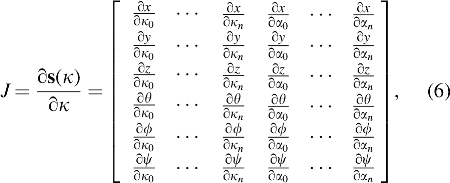
Multiplication of every elements' transformation matrix is an \documentclass{aastex}\usepackage{amsbsy}\usepackage{amsfonts}\usepackage{amssymb}\usepackage{bm}\usepackage{mathrsfs}\usepackage{pifont}\usepackage{stmaryrd}\usepackage{textcomp}\usepackage{portland, xspace}\usepackage{amsmath, amsxtra}\usepackage{upgreek}\pagestyle{empty}\DeclareMathSizes{10}{9}{7}{6}\begin{document} $${ \cal O} ( n )$$ \end{document} operation and it must be computed for every degree of freedom, 2n in this case since each element can control its curvature and twist, resulting in a time complexity of \documentclass{aastex}\usepackage{amsbsy}\usepackage{amsfonts}\usepackage{amssymb}\usepackage{bm}\usepackage{mathrsfs}\usepackage{pifont}\usepackage{stmaryrd}\usepackage{textcomp}\usepackage{portland, xspace}\usepackage{amsmath, amsxtra}\usepackage{upgreek}\pagestyle{empty}\DeclareMathSizes{10}{9}{7}{6}\begin{document} $${ \cal O} ( {n^2} )$$ \end{document} . This can be reduced by precomputing and storing the various transformations, but the problem becomes one of storage and a trade off between communication, storage, and computation in the distributed system.⁴⁰

We distribute the inverse kinematic problem to the robotic material by reducing the number of elements that are allowed to change their curvature and twist at each step. The 2n degree of freedom system is reduced to a 2m degree of freedom system where \documentclass{aastex}\usepackage{amsbsy}\usepackage{amsfonts}\usepackage{amssymb}\usepackage{bm}\usepackage{mathrsfs}\usepackage{pifont}\usepackage{stmaryrd}\usepackage{textcomp}\usepackage{portland, xspace}\usepackage{amsmath, amsxtra}\usepackage{upgreek}\pagestyle{empty}\DeclareMathSizes{10}{9}{7}{6}\begin{document} $$1 \le m \ll n$$ \end{document} and \documentclass{aastex}\usepackage{amsbsy}\usepackage{amsfonts}\usepackage{amssymb}\usepackage{bm}\usepackage{mathrsfs}\usepackage{pifont}\usepackage{stmaryrd}\usepackage{textcomp}\usepackage{portland, xspace}\usepackage{amsmath, amsxtra}\usepackage{upgreek}\pagestyle{empty}\DeclareMathSizes{10}{9}{7}{6}\begin{document} $$n - m$$ \end{document} elements are held rigid during the update. In this scheme, an m-element neighborhood identifies an element to compute the curvature and twist updates using Equation (5). Once the updates are computed, the m-element neighborhood moves down the length of the beam and the process is repeated (Fig. 4). Evaluation of Equation (5) is still linear in time, but now numerically computing the Jacobian is reduced to linear time as well since the forward kinematic function is called only m times.

FIG. 4.

The distributed inverse kinematic method used in our robotic material beam. (A) The 3-link neighborhood at the base computes and executes updates for its degrees of freedom. (B) Communication flows down the length of the beam to the next neighborhood. (C) This process continues until the goal or some other exit criterion is reached.

Figure 5 shows the communication model for a 3-element neighborhood. For a neighborhood of m elements, \documentclass{aastex}\usepackage{amsbsy}\usepackage{amsfonts}\usepackage{amssymb}\usepackage{bm}\usepackage{mathrsfs}\usepackage{pifont}\usepackage{stmaryrd}\usepackage{textcomp}\usepackage{portland, xspace}\usepackage{amsmath, amsxtra}\usepackage{upgreek}\pagestyle{empty}\DeclareMathSizes{10}{9}{7}{6}\begin{document} $$2 ( m - 1 )$$ \end{document} communications are needed to request and receive the curvature, twist, and transformation data from each element in the neighborhood. Once the updates have been completed, \documentclass{aastex}\usepackage{amsbsy}\usepackage{amsfonts}\usepackage{amssymb}\usepackage{bm}\usepackage{mathrsfs}\usepackage{pifont}\usepackage{stmaryrd}\usepackage{textcomp}\usepackage{portland, xspace}\usepackage{amsmath, amsxtra}\usepackage{upgreek}\pagestyle{empty}\DeclareMathSizes{10}{9}{7}{6}\begin{document} $$m - 1$$ \end{document} communications are needed to update curvatures and twists in the neighborhood and \documentclass{aastex}\usepackage{amsbsy}\usepackage{amsfonts}\usepackage{amssymb}\usepackage{bm}\usepackage{mathrsfs}\usepackage{pifont}\usepackage{stmaryrd}\usepackage{textcomp}\usepackage{portland, xspace}\usepackage{amsmath, amsxtra}\usepackage{upgreek}\pagestyle{empty}\DeclareMathSizes{10}{9}{7}{6}\begin{document} $$n - 1$$ \end{document} communications are needed to update transformation matrices of each element. Since we assume \documentclass{aastex}\usepackage{amsbsy}\usepackage{amsfonts}\usepackage{amssymb}\usepackage{bm}\usepackage{mathrsfs}\usepackage{pifont}\usepackage{stmaryrd}\usepackage{textcomp}\usepackage{portland, xspace}\usepackage{amsmath, amsxtra}\usepackage{upgreek}\pagestyle{empty}\DeclareMathSizes{10}{9}{7}{6}\begin{document} $$n \ll m$$ \end{document} for the embedded system, the communication complexity is on the order of \documentclass{aastex}\usepackage{amsbsy}\usepackage{amsfonts}\usepackage{amssymb}\usepackage{bm}\usepackage{mathrsfs}\usepackage{pifont}\usepackage{stmaryrd}\usepackage{textcomp}\usepackage{portland, xspace}\usepackage{amsmath, amsxtra}\usepackage{upgreek}\pagestyle{empty}\DeclareMathSizes{10}{9}{7}{6}\begin{document} $${ \cal O} ( n )$$ \end{document} .

FIG. 5.

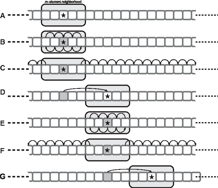
The communication model used in this robotic material. (A) An m-element neighborhood is established and the central element is identified (labeled with a star). (B) The central element collects state information from the neighborhood, computes updates to these degrees of freedom, and sends this information back to elements in the neighborhood. (C) The information is propagated along the length of the beam. (D) Communication flows down the length of the beam and a new m-element neighborhood is established. (E–G) The process continues along the length of the beam.

Results

The multisegment shape-changing material consisting of variable stiffness elements (Related work section), each equipped with a network computing element, is shown in Figure 6. Each computing element provides two functions. First, it measures and controls the temperature of its variable stiffness actuator in a feedback control loop.²⁰ Second, it is part of a distributed computer calculating the required stiffness of its element to reach a desired pose for the beam (Forward and Inverse Kinematics section).

FIG. 6.

Variable stiffness elements are assembled into a beam using acrylic ribs. Small PCBs are attached to each element and are connected to neighboring elements (A). Close-up of an individual element (B). The beam from (A) enclosed into foam with a rubber coating (C). PCB, printed circuit board.

To understand the relationship between stiffness, required time, and required energy, we model the temperature of the variable stiffness element during the Joule heating process so that we can accurately predict the temperature of elements during the operation. The beam is modeled using finite element analysis and compared with the actual heat up times observed in variable stiffness elements. The material properties used are from Ref.³⁸ for polycaprolactone, and standard material properties of acrylic and silicone are from the SolidWorks material library. Joule heating is modeled as 1 W into polycaprolactone faces, touching the acrylic jig with free convection for external faces of the silicone casing. All components are initially at room temperature. Figure 7 shows the correlation between our model and five different beam segments as they are heated up.

FIG. 7.

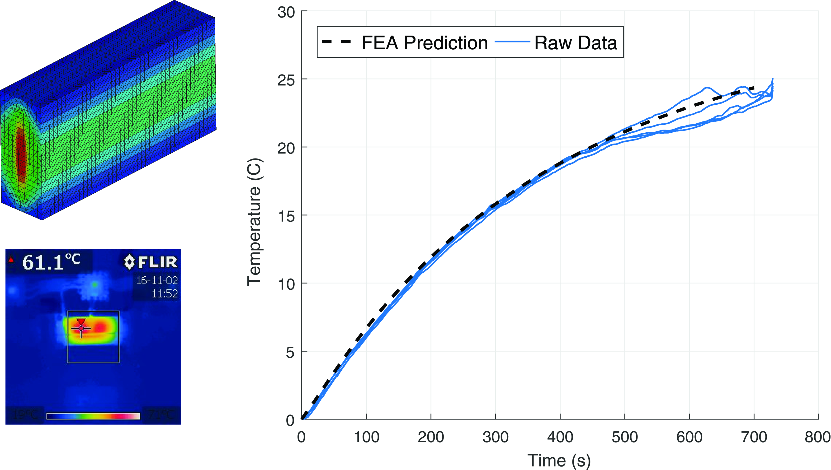
Top left: Finite element simulation predicts the temperature rise and fall times of variable stiffness elements. Right: Comparison of model prediction with experimental data for five different variable stiffness elements. Bottom left: An infrared image showing heat distribution over the length of the element. Color images available online at www.liebertpub.com/soro

Figure 8 compares the required computational time for computing inverse kinematics using centralized and proposed distributed approaches for beams with up to 10,000 elements. For each trial, the beam starts from a straight profile and tries to align with a reachable random goal. For these trials, the goal is the position and orientation of the beam's tip. Trials were terminated when the goal was met within a given tolerance, a local minimum was reached, or the trial exceeded a maximum number of iterations.

FIG. 8.

Average run time using a centralized approach for inverse kinematics (blue) and the distributed method (red) described above. The distributed method grows with \documentclass{aastex}\usepackage{amsbsy}\usepackage{amsfonts}\usepackage{amssymb}\usepackage{bm}\usepackage{mathrsfs}\usepackage{pifont}\usepackage{stmaryrd}\usepackage{textcomp}\usepackage{portland, xspace}\usepackage{amsmath, amsxtra}\usepackage{upgreek}\pagestyle{empty}\DeclareMathSizes{10}{9}{7}{6}\begin{document} $${ \cal O} ( n )$$ \end{document} compared with the \documentclass{aastex}\usepackage{amsbsy}\usepackage{amsfonts}\usepackage{amssymb}\usepackage{bm}\usepackage{mathrsfs}\usepackage{pifont}\usepackage{stmaryrd}\usepackage{textcomp}\usepackage{portland, xspace}\usepackage{amsmath, amsxtra}\usepackage{upgreek}\pagestyle{empty}\DeclareMathSizes{10}{9}{7}{6}\begin{document} $${ \cal O} ( {n^2} )$$ \end{document} growth of the centralized method. Color images available online at www.liebertpub.com/soro

For the proposed distributed method, we see linear growth when computing the update expressed in Equation (5). Adding elements to the beam increases the number of total computations, whereas the computation performed at each individual node remains constant. This is in contrast to the centralized approach, which exhibits exponential growth with growing number of elements. Due to exponential time requirements, we stopped evaluation of the centralized inverse kinematic solution at N = 1000.

To compare the centralized solution with the distributed solution, we chose 10 beam configurations and used the tip positions as goals for each method using a random initial condition this time. Figure 9A shows 10 different beam configurations used in this comparison. For each configuration, we ran the centralized method and distributed method 100 times and compared how each did at finding a solution for the given goal pose. Configurations a through f represent configurations where curvature and twist are constant or vary continuously over the length of the beam, whereas configurations g through j represent configurations where the curvature and twist are discontinuous. Configurations d and e represent the extremes of the beam's workspace. Figure 9B shows that solutions provided by the distributed algorithm are as good or slightly better, in a few cases, than the centralized version of the algorithm.

FIG. 9.

(A) The 10 configurations used to evaluate the effectiveness of the distributed inverse kinematic algorithm compared with the centralized version. Configurations a through f have constant or continuous variations of curvature and twist, while the remaining configurations have discontinuous variations in curvature and twist. (B) A comparison of solutions found for each case. The light gray dots show individual results of each trial, while the large dots show the average. In general, the distributed algorithm does as well or slightly better than the centralized version. Color images available online at www.liebertpub.com/soro

To better understand the difference in solution quality, Figure 10 shows the solutions found for case g in the Cartesian space. All solutions for the distributed case fall on a straight line, while solutions from the centralized case are clustered in a tight grouping near the goal. Solutions from the distributed case also cover a larger space of the beam's self-motion, while the centralized results seem to tend toward the same solution. When a solution is not found, the failure cases from the centralized version are much more erratic and farther away from the goal pose. Failures from the distributed case are still in line with the solution and remain closer to the goal pose.

FIG. 10.

A comparison of solutions found using the distributed algorithm (A) and the centralized algorithm (B) for configuration g, shown in green. All solutions (light gray lines) from the distributed algorithm fall in a line, while all solutions from the centralized algorithm cluster around the same general area. The final pose of each position is indicated by gray dots. Color images available online at www.liebertpub.com/soro

To calibrate for differences between variable stiffness elements due to manufacturing, we measure the curvature of the beam as a function of temperature under a constant load. It is this information that is used by a local controller to set the temperature that corresponds to the curvature that the inverse kinematic solution prescribes.

Friction in our tabletop setup is an external force that is implementation specific and is also easily accounted for in the distributed nature of the material. Elements at the tip of the beam experience a greater curvature than the elements at the base for a given load; in this case, a 500-g weight was hung from the tendons. Figure 11 shows the curvature versus temperature profile of the beam and, equivalently, the range of motion of the beam. Differences in curvature are due to manufacturing differences. For example, elements 2 and 4 in Figure 11A exhibit very similar curvature-to-temperature relationships when bent in the positive direction, but vary dramatically from other elements, which tend to bend less. Specifically, elements 2 and 4 tend to bend up to double as much for the same temperatures as elements 0 and 3 (0.2 vs. 0.1 at 48°C). The same elements that behave similar in the positive direction vary strongly from each other when subjected to negative curvature. For example, element 4 bends almost five times stronger than element 3 at 48°C. As the resulting behavior is strongly nonlinear, it eludes quantification in terms of mean and standard deviation. Rather, we are using the experimental values reported in Figure 11 in a lookup table to select an appropriate temperature for each element based on a desired curvature.

FIG. 11.

To evaluate the curvature that each element can achieve under load, we heat the entire beam while applying a constant load to one of the tendons. (A) Average curvature versus temperature profiles for static load tests using a 500-g weight. (B) Shown in an alternate form, the workspace of our shape-changing beam under constant load. Color images available online at www.liebertpub.com/soro

Finally, we demonstrate the beam's ability to reach and maintain a desired pose obtained through the distributed inverse kinematic algorithm. Figure 12 shows the final curvature achieved by the beam over a sample trial. Here, accuracy of the final pose depends on repeatability of the temperature-dependent curvature of all individual elements (Fig. 11A) and propagation of error along the kinematic chain.

FIG. 12.

Experimental snapshots of moving the beam from an arbitrary start position to a desired goal and the effective end position that the beam reached. The beam position was recorded using an overhead vision system. Color images available online at www.liebertpub.com/soro

Discussion

This article's computational focus is on inverse kinematic algorithms for the tip of the beam to reach a desired pose. We chose this problem as it is computationally hard and scales poorly for large beams when implemented in a centralized manner. The output of the resulting algorithm is a curvature profile consisting of desired curvatures for each element in the beam. Controlling the beam to assume this curvature profile can be achieved in linear time as each element simply needs to control its temperature/curvature accordingly. We note that most practical problems will only require such a solution for shape change.

The range of motion of the robotic material is limited by the construction of various composite parts. A composite can only bend along its centerline, leading to compression and buckling in its periphery. Motion is further impeded by integration of heating, sensing, and computation elements, which are often not flexible. Although other manufacturing techniques such as Shape Deposition Manufacturing⁴¹ might lead to improved results, embedding rigid components into a soft material is still a challenge. Using substrates with gradually varying stiffness is a possible way to embed rigid components into soft materials⁴² without severe stress concentrations, although reducing the range of motion that an otherwise soft material could achieve.

An additional challenge is routing power and communication, the equivalents of vascular networks and the nervous system in biological systems. Embedding of interconnects between each node could be solved using a technique whereby the base polymers are functionalized with a coating of copper,⁴³ resulting in a part that could be populated in a modified circuit board assembly machine and does not require the integration of printed circuit boards or cables. Yet, high-power applications such as Joule heating will still require the integration of multistrand copper wires to deliver the required energy. Although there exist other ways to achieve variable stiffness, each comes with similar problems such as routing of pneumatic or hydraulic hoses.

Another drawback of an implementation with a single variable stiffness element is that positive and negative curvatures must be set in separate steps. This burden could be minimized by shifting the application of the bending moments directly into the material, through the use of shape memory alloys or, optimally, the equivalent to a natural hydrostat. Implementing such actuators comes with additional manufacturing challenges and functional impediments. For example, generating the required torque with two pneumatic bending actuators mounted at either side introduces additional constraints, dramatically reducing the range of motion.

For our specific implementation, there are schemes for setting multiple curvatures at once, although with more communication overhead due to the additional coordination that such approaches require. For example, all elements with either positive or negative curvature could begin their heating process at the same time. As the load is applied and elements reach their desired curvatures, their heating could be turned off, while the other elements continue to heat up and set their curvatures. This scheme would require significantly more communication overhead as elements would need to communicate curvature rates and actuators would need to respond so that element curvatures are set properly.

Conclusions

We show that the distributed inverse kinematic algorithm requires only constant time computation per element, which allows us to implement the shape-changing beam as a material, that is, from identical elements whose computational capabilities are independent of the beam's size. This investigation demonstrates that designing a material that can change its shape autonomously is a codesign problem in which each component—sensing, actuation, computation, and communication—is strongly affected by geometric and dynamical properties of any other component. Nature has mastered this codesign problem brilliantly, as exhibited by the octopus arm and other muscular hydrostat systems with embedded neural computation. By taking inspiration from these mechanisms, we join Webb⁴⁴ in wondering whether engineering integration can also generate hypotheses for the functioning of the biological system. For example, the distributed computation presented here requires only a constant amount of computation per length of element and is therefore likely to require a constant amount of neurons. Similarly, computation travels along the length of the beam, each time leading to incremental movements toward the desired goal, which is similar to activation patterns in the octopus arm.^45,46 While not fitting any disciplinary mold, integration of sensing, actuation, computation, and communication might therefore be of equal intellectual merit than deciphering the functions of equivalent biological systems, whose underlying principles we still have not fully understood.

Footnotes

Acknowledgment

This work has been supported by AFOSR, program manager Byung-Lip “Les” Lee. The authors are grateful for this support.

Author Disclosure Statement

No competing financial interests exist.

References

Kier

, Smith

. Tongues, tentacles and trunks: the biomechanics of movement in muscular-hydrostats. Zool J Linnean Soc, 1985; 83:307–324.

Graziadei

Muscle receptors in cephalopods. Proc R Soc Lond B Biol Sci, 1965; 161:392–402.

Sumbre

, Gutfreund

, Fiorito

, et al. Control of octopus arm extension by a peripheral motor program. Science, 2001; 293:1845–1848.

Hochner

How nervous systems evolve in relation to their embodiment: what we can learn from octopuses and other molluscs. Brain Behav Evol, 2013; 82:19–30.

Gutfreund

, Matzner

, Flash

, et al. Patterns of motor activity in the isolated nerve cord of the octopus arm. Biol Bull, 2006; 211:212–222.

Chirikjian

Hyper-redundant manipulator dynamics: a continuum approximation. Adv Robot, 1994; 9:217–243.

Jones

, Walker

. Practical kinematics for real-time implementation of continuum robots. IEEE Trans Robot, 2006; 22:1087–1099.

McEvoy

, Correll

. Materials that couple sensing, actuation, computation, and communication. Science, 2015; 347:1261689.

Correll

, Heckman

. Materials that make robots smart. In International Symposium on Robotics Research (ISRR). Chile: Puerto Varas, 2017.

10.

Messenger

JB.

Cephalopod chromatophores: neurobiology and natural history. Biol Rev, 2001; 76:473–528.

11.

Hardcastle

, Mann

. Study of large bowel peristalsis. Gut, 1968; 9:512.

12.

Thill

, Etches

, Bond

et al. Morphing skins. Aeron J, 2008; 112:117–139.

13.

Barbarino

, Bilgen

, Ajaj

et al. A review of morphing aircraft. J Intell Mater Syst Struct, 2011; 22:823–877.

14.

Vasista

, Tong

, Wong

. Realization of morphing wings: a multidisciplinary challenge. J Aircraft, 2012; 49:11–28.

15.

Gandhi

, Kang

. Beams with controllable flexural stiffness. Smart Mater Struct, 2007; 16:1179–1184.

16.

Murray

, Gandhi

. Multi-layered controllable stiffness beams for morphing: energy, actuation force, and material strain considerations. Smart Mater Struct, 2010; 19:11.

17.

Brown

, Rodenberg

, Amend

, et al. Universal robotic gripper based on the jamming of granular material. Proc Natl Acad Sci, 2010; 107:18809–18814.

18.

, Yao

, Tauber

, et al. jamSheets: thin interfaces with tunable stiffness enabled by layer jamming. In Proceedings of the 8th International Conference on Tangible, Embedded and Embodied Interaction. Munich, Germany, ACM, 2014, pp. 65–72.

19.

Shan

, Lu

, Majidi

. Soft-matter composites with electrically tunable elastic rigidity. Smart Mater Struct, 2013; 22:085005.

20.

McEvoy

, Correll

. Shape change through programmable stiffness. In International Symposium on Experimental Robotics (ISER). Morocco: Marrakech, 2014.

21.

Shanmuganathan

, Capadona

, Rowan

et al. Biomimetic mechanically adaptive nanocomposites. Prog Polym Sci, 2010; 35:212–222.

22.

Majidi

, Wood

. Tunable elastic stiffness with microconfined magnetorheological domains at low magnetic field. Appl Phys Lett, 2010; 97:164104.

23.

Chen

, Liao

. Design, testing and control of a magnetorheological actuator for assistive knee braces. Smart Mater Struct, 2010; 19:035029.

24.

Varga

, Filipcsei

, Zrnyi

. Magnetic field sensitive functional elastomers with tuneable elastic modulus. Polymer, 2006; 47:227–233.

25.

Pratt

, Williamson

. Series elastic actuators. In Intelligent Robots and Systems 95. 1995. IEEE/RSJ International Conference on “Human Robot Interaction and Cooperative Robots,” Proceedings. Vol. 1, IEEE, 1995, pp. 399–406.

26.

Webster

, Jones

. Design and kinematic modeling of constant curvature continuum robots: a review. Int J Robot Res, 2010; 29:1661–1683.

27.

Yim

, Zhang

, Duff

. Modular robots. Spectrum IEEE, 2002; 39:30–34.

28.

Correll

, Onal

, Liang

, et al. Soft autonomous materials—using active elasticity and embedded distributed computation. In 12th International Symposium on Experimental Robotics, Springer Tracts in Advanced. New Delhi, India, 2014, pp. 227–240.

29.

Marchese

, Konrad

, Onal

, et al. Design, curvature control, and autonomous positioning of a soft and highly compliant 2D robotic manipulator. In 2014 IEEE International Conference on Robotics and Automation. Hong Kong, China, IEEE, 2014.

30.

Robertson

, Paik

. New soft robots really suck: vacuum-powered systems empower diverse capabilities. Sci Robot, 2017; 2:eaan6357.

31.

Tolley

, Shepherd

, Mosadegh

, et al. A resilient, untethered soft robot. Soft Robot, 2014; 1:213–223.

32.

Takashima

, Rossiter

, Mukai

. Mckibben artificial muscle using shape-memory polymer. Sens Actuat A Phys, 2010; 164:116–124.

33.

Abelson

, Allen

, Coore

, et al. Amorphous computing. Commun ACM, 2000; 43:74–82.

34.

Beal

, Dulman

, Usbeck

, et al. Organizing the aggregate: languages for spatial computing. In: Formal and Practical Aspects of Domain-Specific Languages: Recent Developments. Hershey, PA: IGI Global, 2012, p. 436.

35.

Suomela

Survey of local algorithms. ACM Comput Surv, 2013; 45:24.

36.

McEvoy

, Correll

. Thermoplastic variable stiffness composites with embedded, networked sensing, actuation, and control. J Comp Mater, 2014; 49:1799–1808.

37.

McEvoy

, Correll

Distributed inverse kinematics for shape-changing robotic materials. Procedia Technology, Proceedings of International Conference on System-Integrated Intelligence. Paderborn, Germany, 2016, pp. 4–11.

38.

Averous

, Moro

, Dole

, et al. Properties of thermoplastic blends: starch–polycaprolactone. Polymer, 2000; 41:4157–4167.

39.

Buss

SR.

Introduction to inverse kinematics with jacobian transpose, pseudoinverse and damped least squares methods. IEEE J Robot Autom, 2004; 17:16.

40.

Hosseinmardi

, Mysore

, Farrow

, et al. Distributed spatiotemporal gesture recognition in sensor arrays. ACM Trans Auton Adap Syst, 2015; 10:17.

41.

Merz

, Prinz

, Ramaswami

, et al. Shape Deposition Manufacturing. Engineering Design Research Center, Carnegie Mellon University, 1994.

42.

Menguc

, Park

, Pei

, et al. Wearable soft sensing suit for human gait measurement. Int J Robot Res, 2014; 33:1748–1764.

43.

Islam

, Hansen

, Tang

et al. Process chains for the manufacturing of molded interconnect devices. Int J Adv Manuf Technol, 2009; 42:831–841.

44.

Webb

Can robots make good models of biological behaviour?. Behav Brain Sci, 2001; 24:1033–1050.

45.

Gutfreund

, Flash

, Yarom

, et al. Organization of octopus arm movements: a model system for studying the control of flexible arms. J Neurosci, 1996; 16:7297–7307.

46.

Gutfreund

, Flash

, Fiorito

, et al. Patterns of arm muscle activation involved in octopus reaching movements. J Neurosci, 1998; 18:5976–5987.