Modeling soft robots that move on surfaces is challenging from a variety of perspectives. A recent formulation by Bergou et al. of a rod theory that exploits new developments in discrete differential geometry offers an attractive, numerically efficient avenue to help overcome some of these challenges. Their formulation is an example of a discrete elastic rod theory. In this article, we consider a planar version of Bergou et al.'s theory and, with the help of recent works on Lagrange's equations of motion for constrained systems of particles, show how it can be used to model soft robots that are composed of segments of soft material folded and bonded together. We then use our formulation to examine the dynamics of a caterpillar-inspired soft robot that is actuated using shape memory alloys and exploits stick-slip friction to achieve locomotion. After developing and implementing procedures to prescribe the parameters for components of the soft robot, we compare our calibrated model to the experimental behavior of the caterpillar-inspired soft robot.
Introduction
The field of soft robots has emerged as a prominent research area in mechanics in the past decade. The function of these soft robots ranges from soft gripping devices such as Galloway et al.1 and Laschi et al.'s octopus2 with fully functional extending and grabbing tentacles to locomoting devices such as the worm-like robot developed by Seok et al.3 and the caterpillar-inspired robot developed by Trimmer and colleagues.4 While much of the work in soft robots focuses on design and construction, works on the challenging tasks of developing and analyzing models for these machines are far fewer in number.5–11 Models that have appeared in the literature use finite element methods or rod-based theories to model the robot (cf.8,12,13 and references therein). Developing tractable finite element models that are validated with soft robot prototypes is challenging and often involves some type of model reduction (cf.5). Notable examples of this work include Renda et al.'s model for an underwater soft robot.10 Because of the challenges in modeling frictional contact, developing, validating, and analyzing models for soft robots that are designed to grip objects or locomote on rough terrains are difficult.
Nonetheless, a new avenue to develop models for soft robots has become available due to Bergou et al.'s recent formulation of a discrete elastic rod theory.14–16 Their formulation, which we refer to as a discrete elastic rod (DER), is computationally efficient and can model the three-dimensional dynamics of elastic and viscoelastic rods that are capable of bending, stretching, and twisting. The computational advantages of the DER formulation over traditional approaches, such as finite element models, lumped parameter models, or continuous rod models, make it ideal for use in analyzing soft robots. These advantages include generation of ordinary differential equations for the motion of the soft robot that can interface with control schemes and contact algorithms, ability to incorporate a hierarchy of rod models, and ease of interpretation and measurement of kinematical quantities. We also take this opportunity to note that discrete elastic rod formulations are also used to analyze assembly processes for cables (cf.17–19).
The purpose of the present article is to examine a planar version of DER that is capable of modeling locomoting soft robots as a branched structure in frictional contact with a surface and then use the formulation to model the dynamics of a soft robot test bed. For brevity, we refer to this formulation as a planar discrete elastic rod (PDER). The soft robot that we examine is a caterpillar-inspired robot shown in Figure 1. Using the PDER model, we are able to examine the efficacy of actuation strategies for the robot as it locomotes on a rough horizontal surface. Complementing Bergou et al.'s original works,14–16 we derive formulations of the equations of motion for the PDER by taking advantage of recent works on the formulation of Lagrange's equations of motion for a discrete set of particles.20,21 We also explore a novel folding strategy to develop models for soft robots composed of multiple shape memory alloy (SMA) actuators bonded together such as those shown in Figure 1.
Caterpillar-inspired robot made out of six SMA actuator segments connected in series, with embedded flexible circuit and battery packs on top. The inset image shows a schematic of the assembly process for a single actuator segment. SMA, shape memory alloy. Color images are available online.
As in earlier works on locomotion,12,22 the locomotion in the soft robots we analyze is a product of stick-slip friction induced by changing the intrinsic curvature of the rod-like structure that is being used to model the SMA actuator. However, in contrast to earlier work, which involved a quasi-static analysis of an elastica with an attached mass at one of its ends12 and a multibody dynamics model for a caterpillar-inspired robot,23 in this study we analyze the dynamics of the actuator using the PDER formulation. The PDER formulation also provides a set of ordinary differential equations for the discrete model of the soft robot. In ongoing work, these equations are being used to design distributed feedback control strategies.
An outline of the article is as follows. In the next section, ingredients needed to formulate a planar theory of a discrete elastic rod are presented. The theory is a specialization of Bergou et al.'s formulation for an extensible rod that resists bending and torsion.14–16 For the planar case, we are able to restrict attention to bending and stretching and the DER formulation simplifies dramatically. Once the kinematical preliminaries have been presented, we turn to a discussion of mass matrices and inertias in Prescribing Masses and Inertias section and forces and elastic potential energies in Forces and Energies section. Our treatment in the latter section closely follows a recently published primer on DER.24 With the preliminaries taken care of, we then turn to presenting Lagrange's equations of motion for a rod that is free to move on a surface (and is consequently subject to external constraints). In this study, we take advantage of recent works20,21,25 on Lagrange's equations of motion for systems of particles to formulate the equations in a systematic manner. In the Constraining a Discrete Elastic Rod section we apply the ideas from these works to consider folding a rod so the PDER is capable of modeling tree-like structures. This capability is needed if we are to be able to model soft robots such as the one shown in Figure 1.
The PDER formulation that incorporates folded rods and branched tree-like structures is then used to model an SMA-actuated soft robot. First, however, we develop and implement strategies to determine the parameters of the PDER model. These parameters include intrinsic curvature and Young's moduli, both of which are functions of time. Next, we consider the caterpillar-inspired soft robot shown in Figure 1. The design of the soft robot is based on measurements of caterpillar kinematics performed by Trimmer and Issberner,26 where actuator segments are connected in series to mimic body segments of a caterpillar that are actuated from rear to front to result in forward locomotion. In this study, we model the segments as connected SMA actuators and model the entire robot as a tree-like branched structure. Mimicking the actual soft robot, we are able to demonstrate that locomotion can be achieved by actuating the segments in a particular order. Our model also enables the study of the efficiency of different actuation schemes.
Additional details on the fabrication and testing of the SMA actuators are presented in Appendix A.
A Planar Discrete Elastic Rod
We consider Bergou et al.'s14–16 formulation of a discrete elastic rod. Their theory is sufficiently general to model the stretching, torsional, and flexural deformations of an extensible, flexible elastic rod. In this section of the article, we restrict the theory to the planar case. Thus, the rod is free to move on a plane, and the torsional deformation of the rod is ignored. The resulting simplifications to Bergou et al.'s formulation are considerable, and we refer to the theory as PDER in the sequel.
In a discrete elastic rod formulation, the centerline of the rod is discretized into a series of n nodes (or vertices) that are connected by n − 1 segments (edges), where n is an integer. The higher the n, the more refined the discretization of the rod. The position vectors of the nodes that define the edges are denoted by x0, …, xn − 1 (cf. Fig. 2). The edge vector ei and the associated unit vector ti are defined as follows:
In this study, and in the sequel, a subscript is used to denote quantities associated with a vertex (e.g., xk), and a superscript is used to denote quantities associated with an edge (e.g., ei). For the PDER, it is convenient to identify the material vector (director) \documentclass{aastex}\usepackage{amsbsy}\usepackage{amsfonts}\usepackage{amssymb}\usepackage{bm}\usepackage{mathrsfs}\usepackage{pifont}\usepackage{stmaryrd}\usepackage{textcomp}\usepackage{portland, xspace}\usepackage{amsmath, amsxtra}\usepackage{upgreek}\pagestyle{empty}\DeclareMathSizes{10}{9}{7}{6}\begin{document}
$${\bf m}_1^k$$
\end{document} with the unit normal vector for each edge and the material vector (director) \documentclass{aastex}\usepackage{amsbsy}\usepackage{amsfonts}\usepackage{amssymb}\usepackage{bm}\usepackage{mathrsfs}\usepackage{pifont}\usepackage{stmaryrd}\usepackage{textcomp}\usepackage{portland, xspace}\usepackage{amsmath, amsxtra}\usepackage{upgreek}\pagestyle{empty}\DeclareMathSizes{10}{9}{7}{6}\begin{document}
$${\bf m}_2^k = {{\bf E}_3}$$
\end{document} with the out-of-plane direction:
\documentclass{aastex}\usepackage{amsbsy}\usepackage{amsfonts}\usepackage{amssymb}\usepackage{bm}\usepackage{mathrsfs}\usepackage{pifont}\usepackage{stmaryrd}\usepackage{textcomp}\usepackage{portland, xspace}\usepackage{amsmath, amsxtra}\usepackage{upgreek}\pagestyle{empty}\DeclareMathSizes{10}{9}{7}{6}\begin{document}
\begin{align*}
{\bf m}_1^k = {{\bf n}^k} = {{\bf E}_3} \times {{\bf t}^k} , \qquad {\bf m}_2^k = {{\bf E}_3}. \tag{2.2}
\end{align*}
\end{document}
Thus, \documentclass{aastex}\usepackage{amsbsy}\usepackage{amsfonts}\usepackage{amssymb}\usepackage{bm}\usepackage{mathrsfs}\usepackage{pifont}\usepackage{stmaryrd}\usepackage{textcomp}\usepackage{portland, xspace}\usepackage{amsmath, amsxtra}\usepackage{upgreek}\pagestyle{empty}\DeclareMathSizes{10}{9}{7}{6}\begin{document}
$$\left\{ {{{\bf t}^k} , {{\bf n}^k} , {{\bf E}_3}} \right\} $$
\end{document} is an orthonormal triad of vectors. The turning angle can be used to relate the triads at adjacent edges:
\documentclass{aastex}\usepackage{amsbsy}\usepackage{amsfonts}\usepackage{amssymb}\usepackage{bm}\usepackage{mathrsfs}\usepackage{pifont}\usepackage{stmaryrd}\usepackage{textcomp}\usepackage{portland, xspace}\usepackage{amsmath, amsxtra}\usepackage{upgreek}\pagestyle{empty}\DeclareMathSizes{10}{9}{7}{6}\begin{document}
\begin{align*}
{{\bf t}^k} = \cos \left( {{ \varphi _k}} \right) {{\bf t}^{k - 1}} + \sin \left( {{ \varphi _k}} \right) {{\bf n}^{k - 1}} , \quad {{\bf n}^k} = \cos \left( {{ \varphi _k}} \right) {{\bf n}^{k - 1}} - \sin \left( {{ \varphi _k}} \right) {{\bf t}^{k - 1}}. \tag{2.3}
\end{align*}
\end{document}
Three vertices xk−1, xk, and xk+1 of a PDER. This figure also illustrates the pairs of unit vectors \documentclass{aastex}\usepackage{amsbsy}\usepackage{amsfonts}\usepackage{amssymb}\usepackage{bm}\usepackage{mathrsfs}\usepackage{pifont}\usepackage{stmaryrd}\usepackage{textcomp}\usepackage{portland, xspace}\usepackage{amsmath, amsxtra}\usepackage{upgreek}\pagestyle{empty}\DeclareMathSizes{10}{9}{7}{6}\begin{document}
$$\left\{ {{{\bf t}^k} , {{\bf n}^k}} \right\} $$
\end{document} associated with the edges and the turning angle φk. The unit vectors E1 and E2 define an inertial frame. PDER, planar discrete elastic rod. Color images are available online.
Associated with each vertex, we define the length ℓk of the Voronoi region:
where k = 1, …, n − 2.
For the discrete elastic rod, a signed discrete integrated curvature κk can be defined at the kth vertex:
\documentclass{aastex}\usepackage{amsbsy}\usepackage{amsfonts}\usepackage{amssymb}\usepackage{bm}\usepackage{mathrsfs}\usepackage{pifont}\usepackage{stmaryrd}\usepackage{textcomp}\usepackage{portland, xspace}\usepackage{amsmath, amsxtra}\usepackage{upgreek}\pagestyle{empty}\DeclareMathSizes{10}{9}{7}{6}\begin{document}
\begin{align*}
{ \kappa _k } = { \frac { 2 \sin \left( { { \varphi _k } } \right) } { 1 + \cos \left( { { \varphi _k } } \right) } } = 2 { \mkern 1mu } { \rm { tan } } \left( { \frac { { { \varphi _k } } } { 2 } } \right) , \tag { 2.5 }
\end{align*}
\end{document}
where φk is the turning angle at the kth vertex. In comparison to the curvature of a continuous curve, κk can be easily measured in soft robot actuators where optical methods are used to track a set of discrete points.23 The curvature κk is dimensionless and, as shown in Figure 3, this function is not defined when the edges are antiparallel. We observe that
In this equation, \documentclass{aastex}\usepackage{amsbsy}\usepackage{amsfonts}\usepackage{amssymb}\usepackage{bm}\usepackage{mathrsfs}\usepackage{pifont}\usepackage{stmaryrd}\usepackage{textcomp}\usepackage{portland, xspace}\usepackage{amsmath, amsxtra}\usepackage{upgreek}\pagestyle{empty}\DeclareMathSizes{10}{9}{7}{6}\begin{document}
$$\delta _i^k$$
\end{document} is the Kronecker delta: that is, \documentclass{aastex}\usepackage{amsbsy}\usepackage{amsfonts}\usepackage{amssymb}\usepackage{bm}\usepackage{mathrsfs}\usepackage{pifont}\usepackage{stmaryrd}\usepackage{textcomp}\usepackage{portland, xspace}\usepackage{amsmath, amsxtra}\usepackage{upgreek}\pagestyle{empty}\DeclareMathSizes{10}{9}{7}{6}\begin{document}
$$\delta _i^k = 1$$
\end{document} if i = k and is otherwise 0.
The discrete curvature κk as a function of the turning angle φk. When φk = π, the edges of the rod are coincident and, as φk passes through π, the edges intersect. Such behavior is nonphysical and is penalized by the forces in the rod which, in proportion to κk, become unbounded as φk → π. Color images are available online.
The discrete integrated curvature vector κkE3 at the vertex xk is used to quantify the bending strain of the rod:
\documentclass{aastex}\usepackage{amsbsy}\usepackage{amsfonts}\usepackage{amssymb}\usepackage{bm}\usepackage{mathrsfs}\usepackage{pifont}\usepackage{stmaryrd}\usepackage{textcomp}\usepackage{portland, xspace}\usepackage{amsmath, amsxtra}\usepackage{upgreek}\pagestyle{empty}\DeclareMathSizes{10}{9}{7}{6}\begin{document}
\begin{align*}
{ \kappa _k } { { \bf E } _3 } = { \frac { 2 { { \bf t } ^ { k - 1 } } \times { { \bf t } ^k } } { 1 + { { \bf t } ^ { k - 1 } } \cdot { { \bf t } ^k } } } . \tag { 2.7 }
\end{align*}
\end{document}
The representation (2.7) can be considered a specialization of the three-dimensional curvature vector to the PDER. The curvature κk can be considered as a planar version of the vertex-based material curvatures \documentclass{aastex}\usepackage{amsbsy}\usepackage{amsfonts}\usepackage{amssymb}\usepackage{bm}\usepackage{mathrsfs}\usepackage{pifont}\usepackage{stmaryrd}\usepackage{textcomp}\usepackage{portland, xspace}\usepackage{amsmath, amsxtra}\usepackage{upgreek}\pagestyle{empty}\DeclareMathSizes{10}{9}{7}{6}\begin{document}
$${ \kappa _{{k_1}}}$$
\end{document} and \documentclass{aastex}\usepackage{amsbsy}\usepackage{amsfonts}\usepackage{amssymb}\usepackage{bm}\usepackage{mathrsfs}\usepackage{pifont}\usepackage{stmaryrd}\usepackage{textcomp}\usepackage{portland, xspace}\usepackage{amsmath, amsxtra}\usepackage{upgreek}\pagestyle{empty}\DeclareMathSizes{10}{9}{7}{6}\begin{document}
$${ \kappa _{{k_2}}}$$
\end{document} introduced in Bergou et al.15 The curvatures \documentclass{aastex}\usepackage{amsbsy}\usepackage{amsfonts}\usepackage{amssymb}\usepackage{bm}\usepackage{mathrsfs}\usepackage{pifont}\usepackage{stmaryrd}\usepackage{textcomp}\usepackage{portland, xspace}\usepackage{amsmath, amsxtra}\usepackage{upgreek}\pagestyle{empty}\DeclareMathSizes{10}{9}{7}{6}\begin{document}
$${ \kappa _{{k_1}}}$$
\end{document} and \documentclass{aastex}\usepackage{amsbsy}\usepackage{amsfonts}\usepackage{amssymb}\usepackage{bm}\usepackage{mathrsfs}\usepackage{pifont}\usepackage{stmaryrd}\usepackage{textcomp}\usepackage{portland, xspace}\usepackage{amsmath, amsxtra}\usepackage{upgreek}\pagestyle{empty}\DeclareMathSizes{10}{9}{7}{6}\begin{document}
$${ \kappa _{{k_2}}}$$
\end{document} are used to formulate bending strains and elastic energy associated with bending. Alternative measures of bending strain are used in polymer dynamics where a worm-like chain model consisting of bead and springs is used to model polymers. These alternative measures include the turning angle φk and (cf.27 and references therein).
For future reference, the variation of κk due to the displacements of the edges of the discrete rod is presented in this study. The following are intermediate results from Jawed et al.24, Chapter 6 that can be used to compute these variations:
One can verify that the variations are orthogonal to E3 as expected. Indeed, for the planar case of interest we can simplify Equation (2.8) using the identities
\documentclass{aastex}\usepackage{amsbsy}\usepackage{amsfonts}\usepackage{amssymb}\usepackage{bm}\usepackage{mathrsfs}\usepackage{pifont}\usepackage{stmaryrd}\usepackage{textcomp}\usepackage{portland, xspace}\usepackage{amsmath, amsxtra}\usepackage{upgreek}\pagestyle{empty}\DeclareMathSizes{10}{9}{7}{6}\begin{document}
\begin{align*}
{{\bf t}^{k - 1}} \times {{\bf t}^k} = ( {{\bf n}^{k - 1}} \cdot {{\bf t}^k} ) {{\bf E}_3} = - ( {{\bf t}^{k - 1}} \cdot {{\bf n}^k} ) {{\bf E}_3}. \tag{2.9}
\end{align*}
\end{document}
Thus, we have the following simplifications of Equation (2.8):
Prescribing Masses and Inertias
Following Bergou et al.,14–16 the mass Mi associated with the ith vertex is the average mass of the edges meeting at this vertex:
For a homogeneous rod with a uniform cross-section in its reference configuration (or reference state),
where ρ0 is the mass density per unit volume in the reference configuration, Ai is the cross-sectional area in the reference configuration, and denotes the length of the ith edge in the reference configuration. If the rod is not homogeneous or of a uniform cross-section, then Mi must be computed using a more primitive prescription:
\documentclass{aastex}\usepackage{amsbsy}\usepackage{amsfonts}\usepackage{amssymb}\usepackage{bm}\usepackage{mathrsfs}\usepackage{pifont}\usepackage{stmaryrd}\usepackage{textcomp}\usepackage{portland, xspace}\usepackage{amsmath, amsxtra}\usepackage{upgreek}\pagestyle{empty}\DeclareMathSizes{10}{9}{7}{6}\begin{document}
\begin{align*}
{M^i} = \int { \int { \int {{ \rho _0}} } } d{x_1}d{x_2}d{x_3} , \qquad \left( {i = 0 , \ldots , n - 2} \right) , \tag{3.3}
\end{align*}
\end{document}
where the integration is performed over the segment of the three-dimensional body that the ith edge is modeling.
The mass moments of inertia associated with the ith edge are defined with the help of volume integrals:
\documentclass{aastex}\usepackage{amsbsy}\usepackage{amsfonts}\usepackage{amssymb}\usepackage{bm}\usepackage{mathrsfs}\usepackage{pifont}\usepackage{stmaryrd}\usepackage{textcomp}\usepackage{portland, xspace}\usepackage{amsmath, amsxtra}\usepackage{upgreek}\pagestyle{empty}\DeclareMathSizes{10}{9}{7}{6}\begin{document}
\begin{align*}
\rho _0^i{I^i} = \int { \int { \int {x_2^2} } } { \rho _0}d{x_1}d{x_2}d{x_3} , \quad \left( {i = 0 , \ldots , n - 2} \right). \tag{3.4}
\end{align*}
\end{document}
Thus, for a segment of length \documentclass{aastex}\usepackage{amsbsy}\usepackage{amsfonts}\usepackage{amssymb}\usepackage{bm}\usepackage{mathrsfs}\usepackage{pifont}\usepackage{stmaryrd}\usepackage{textcomp}\usepackage{portland, xspace}\usepackage{amsmath, amsxtra}\usepackage{upgreek}\pagestyle{empty}\DeclareMathSizes{10}{9}{7}{6}\begin{document}
$$\ell$$
\end{document} of a homogeneous rod with a rectangular cross-section of height h (in the x2 direction) and width w (in the out-of-plane x3 direction):
\documentclass{aastex}\usepackage{amsbsy}\usepackage{amsfonts}\usepackage{amssymb}\usepackage{bm}\usepackage{mathrsfs}\usepackage{pifont}\usepackage{stmaryrd}\usepackage{textcomp}\usepackage{portland, xspace}\usepackage{amsmath, amsxtra}\usepackage{upgreek}\pagestyle{empty}\DeclareMathSizes{10}{9}{7}{6}\begin{document}
\begin{align*}
\rho _0^i { I^i } = { \rho _0 } \ell { \frac { h { w^3 } } { 12 } } = { \frac { { M^i } { w^2 } } { 12 } } . \tag { 3.5 }
\end{align*}
\end{document}
Observe that we have used the definition of the mass Mi of the ith edge to simplify the expression for \documentclass{aastex}\usepackage{amsbsy}\usepackage{amsfonts}\usepackage{amssymb}\usepackage{bm}\usepackage{mathrsfs}\usepackage{pifont}\usepackage{stmaryrd}\usepackage{textcomp}\usepackage{portland, xspace}\usepackage{amsmath, amsxtra}\usepackage{upgreek}\pagestyle{empty}\DeclareMathSizes{10}{9}{7}{6}\begin{document}
$$\rho _0^i{I^i}$$
\end{document}.
This matrix can be used to formulate an expression for the kinetic energy T of the rod:
\documentclass{aastex}\usepackage{amsbsy}\usepackage{amsfonts}\usepackage{amssymb}\usepackage{bm}\usepackage{mathrsfs}\usepackage{pifont}\usepackage{stmaryrd}\usepackage{textcomp}\usepackage{portland, xspace}\usepackage{amsmath, amsxtra}\usepackage{upgreek}\pagestyle{empty}\DeclareMathSizes{10}{9}{7}{6}\begin{document}
\begin{align*}
T = \frac { 1 } { 2 } \mathop \sum \limits_ { k = 0 } ^ { n - 1 } { \left( { \dot { \bf x } _k^T { M_k } { { \dot { \bf x } } _k } } \right) } . \tag { 3.7 }
\end{align*}
\end{document}
where
The mass matrix in Equation (3.6) is always positive definite.
Forces and Energies
For the planar rod theory, we assume that the elastic energy is incorporated into the stretching and bending of the rod; torsion is ignored. The elastic potential energy Ee is a function of the stretching of the edges and the turning angles between the adjacent edges. A simple choice of the function Ee is an additive decomposition of a stretching energy Es and a bending energy Eb:
\documentclass{aastex}\usepackage{amsbsy}\usepackage{amsfonts}\usepackage{amssymb}\usepackage{bm}\usepackage{mathrsfs}\usepackage{pifont}\usepackage{stmaryrd}\usepackage{textcomp}\usepackage{portland, xspace}\usepackage{amsmath, amsxtra}\usepackage{upgreek}\pagestyle{empty}\DeclareMathSizes{10}{9}{7}{6}\begin{document}
\begin{align*}
{E_e} = {E_s} + {E_b}. \tag{4.1}
\end{align*}
\end{document}
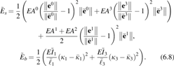
The respective extensional Es and bending Eb elastic energy functions are assumed to be quadratic functions of the strains:
In these expressions, the overbars ornamenting \documentclass{aastex}\usepackage{amsbsy}\usepackage{amsfonts}\usepackage{amssymb}\usepackage{bm}\usepackage{mathrsfs}\usepackage{pifont}\usepackage{stmaryrd}\usepackage{textcomp}\usepackage{portland, xspace}\usepackage{amsmath, amsxtra}\usepackage{upgreek}\pagestyle{empty}\DeclareMathSizes{10}{9}{7}{6}\begin{document}
$$\ell$$
\end{document}k, ej, mi, and κi denote the values of these quantities in a fixed reference configuration, and E denotes the Young's modulus. The moment of inertia in the bending energy is based on the average of the areal moments of inertia:
\documentclass{aastex}\usepackage{amsbsy}\usepackage{amsfonts}\usepackage{amssymb}\usepackage{bm}\usepackage{mathrsfs}\usepackage{pifont}\usepackage{stmaryrd}\usepackage{textcomp}\usepackage{portland, xspace}\usepackage{amsmath, amsxtra}\usepackage{upgreek}\pagestyle{empty}\DeclareMathSizes{10}{9}{7}{6}\begin{document}
\begin{align*}
{ I_i } = \frac { 1 } { 2 } \left( { { I^i } + { I^ { i - 1 } } } \right). \tag { 4.3 }
\end{align*}
\end{document}
This averaged quantity is considered a vertex-based measure. In the sequel, the intrinsic curvature \documentclass{aastex}\usepackage{amsbsy}\usepackage{amsfonts}\usepackage{amssymb}\usepackage{bm}\usepackage{mathrsfs}\usepackage{pifont}\usepackage{stmaryrd}\usepackage{textcomp}\usepackage{portland, xspace}\usepackage{amsmath, amsxtra}\usepackage{upgreek}\pagestyle{empty}\DeclareMathSizes{10}{9}{7}{6}\begin{document}
$${ \bar \kappa _i}$$
\end{document} at the vertex will change depending on the actuation of the SMA actuator that the PDER is modeling. Modeling the actuation using the intrinsic curvature is also a strategy used in models of pneu-net actuators (cf.28).
The force \documentclass{aastex}\usepackage{amsbsy}\usepackage{amsfonts}\usepackage{amssymb}\usepackage{bm}\usepackage{mathrsfs}\usepackage{pifont}\usepackage{stmaryrd}\usepackage{textcomp}\usepackage{portland, xspace}\usepackage{amsmath, amsxtra}\usepackage{upgreek}\pagestyle{empty}\DeclareMathSizes{10}{9}{7}{6}\begin{document}
$${{\bf F}_{{e_i}}}$$
\end{document} acting on the ith vertex can be prescribed by solving an energy balance that equates the negative of the time rate of change of the elastic energy to the combined mechanical power of the forces \documentclass{aastex}\usepackage{amsbsy}\usepackage{amsfonts}\usepackage{amssymb}\usepackage{bm}\usepackage{mathrsfs}\usepackage{pifont}\usepackage{stmaryrd}\usepackage{textcomp}\usepackage{portland, xspace}\usepackage{amsmath, amsxtra}\usepackage{upgreek}\pagestyle{empty}\DeclareMathSizes{10}{9}{7}{6}\begin{document}
$${{\bf F}_{{e_0}}} , \ldots , {{\bf F}_{{e_{n - 1}}}}$$
\end{document}24:
\documentclass{aastex}\usepackage{amsbsy}\usepackage{amsfonts}\usepackage{amssymb}\usepackage{bm}\usepackage{mathrsfs}\usepackage{pifont}\usepackage{stmaryrd}\usepackage{textcomp}\usepackage{portland, xspace}\usepackage{amsmath, amsxtra}\usepackage{upgreek}\pagestyle{empty}\DeclareMathSizes{10}{9}{7}{6}\begin{document}
\begin{align*}
{ \dot E_e} = - \mathop \sum \limits_{i = 0}^{n - 1} {{{\bf F}_{{e_i}}}} \cdot { \dot {\bf x}_i}. \tag{4.4}
\end{align*}
\end{document}
This procedure mimics the definition of conservative forces in systems of particles.21 For the choice of Ee we have selected, it is possible to decompose the force vector at the ith vertex:
\documentclass{aastex}\usepackage{amsbsy}\usepackage{amsfonts}\usepackage{amssymb}\usepackage{bm}\usepackage{mathrsfs}\usepackage{pifont}\usepackage{stmaryrd}\usepackage{textcomp}\usepackage{portland, xspace}\usepackage{amsmath, amsxtra}\usepackage{upgreek}\pagestyle{empty}\DeclareMathSizes{10}{9}{7}{6}\begin{document}
\begin{align*}
{{\bf F}_{{e_i}}} = {{\bf F}_{{s_i}}} + {{\bf F}_{{b_i}}}. \tag{4.5}
\end{align*}
\end{document}
In this study, the force \documentclass{aastex}\usepackage{amsbsy}\usepackage{amsfonts}\usepackage{amssymb}\usepackage{bm}\usepackage{mathrsfs}\usepackage{pifont}\usepackage{stmaryrd}\usepackage{textcomp}\usepackage{portland, xspace}\usepackage{amsmath, amsxtra}\usepackage{upgreek}\pagestyle{empty}\DeclareMathSizes{10}{9}{7}{6}\begin{document}
$${{\bf F}_{{s_i}}}$$
\end{document} is associated with a stretching energy, and the force \documentclass{aastex}\usepackage{amsbsy}\usepackage{amsfonts}\usepackage{amssymb}\usepackage{bm}\usepackage{mathrsfs}\usepackage{pifont}\usepackage{stmaryrd}\usepackage{textcomp}\usepackage{portland, xspace}\usepackage{amsmath, amsxtra}\usepackage{upgreek}\pagestyle{empty}\DeclareMathSizes{10}{9}{7}{6}\begin{document}
$${{\bf F}_{{b_i}}}$$
\end{document} is associated with a bending or flexural energy. These forces can be prescribed by assuming that they satisfy the following energy balance for all motions of the rod:
\documentclass{aastex}\usepackage{amsbsy}\usepackage{amsfonts}\usepackage{amssymb}\usepackage{bm}\usepackage{mathrsfs}\usepackage{pifont}\usepackage{stmaryrd}\usepackage{textcomp}\usepackage{portland, xspace}\usepackage{amsmath, amsxtra}\usepackage{upgreek}\pagestyle{empty}\DeclareMathSizes{10}{9}{7}{6}\begin{document}
\begin{align*}
{ \dot E_s} + { \dot E_b} = - \mathop \sum \limits_{i = 0}^{n - 1} { \left( {{{\bf F}_{{s_i}}} + {{\bf F}_{{b_i}}}} \right) } \cdot { \dot {\bf x}_i}. \tag{4.6}
\end{align*}
\end{document}
After some rearranging, we find that Equation (4.6) can be expressed as
\documentclass{aastex}\usepackage{amsbsy}\usepackage{amsfonts}\usepackage{amssymb}\usepackage{bm}\usepackage{mathrsfs}\usepackage{pifont}\usepackage{stmaryrd}\usepackage{textcomp}\usepackage{portland, xspace}\usepackage{amsmath, amsxtra}\usepackage{upgreek}\pagestyle{empty}\DeclareMathSizes{10}{9}{7}{6}\begin{document}
\begin{align*}
\mathop \sum \limits_{i = 0}^{n - 1} {{{\bf X}_i}} \cdot { \dot {\bf x}}_i = 0. \tag{4.7}
\end{align*}
\end{document}
In this equation,
As Equation (4.7) is assumed to hold true for all motions of the discrete rod, the vectors Xi are independent of \documentclass{aastex}\usepackage{amsbsy}\usepackage{amsfonts}\usepackage{amssymb}\usepackage{bm}\usepackage{mathrsfs}\usepackage{pifont}\usepackage{stmaryrd}\usepackage{textcomp}\usepackage{portland, xspace}\usepackage{amsmath, amsxtra}\usepackage{upgreek}\pagestyle{empty}\DeclareMathSizes{10}{9}{7}{6}\begin{document}
$${ \dot {\bf x}_i}$$
\end{document}, and x0, …, xn – 1 can all be independently varied, we can conclude that
\documentclass{aastex}\usepackage{amsbsy}\usepackage{amsfonts}\usepackage{amssymb}\usepackage{bm}\usepackage{mathrsfs}\usepackage{pifont}\usepackage{stmaryrd}\usepackage{textcomp}\usepackage{portland, xspace}\usepackage{amsmath, amsxtra}\usepackage{upgreek}\pagestyle{empty}\DeclareMathSizes{10}{9}{7}{6}\begin{document}
\begin{align*}
{{\bf X}_k} = {\bf 0} , \qquad \qquad \left( {k = 0 , \ldots , n - 1} \right). \tag{4.9}
\end{align*}
\end{document}
It is now possible to equate the forces to the gradients of the elastic energy.
With the help of Equation (4.8), an expression for the internal force \documentclass{aastex}\usepackage{amsbsy}\usepackage{amsfonts}\usepackage{amssymb}\usepackage{bm}\usepackage{mathrsfs}\usepackage{pifont}\usepackage{stmaryrd}\usepackage{textcomp}\usepackage{portland, xspace}\usepackage{amsmath, amsxtra}\usepackage{upgreek}\pagestyle{empty}\DeclareMathSizes{10}{9}{7}{6}\begin{document}
$${{\bf F}_{{s_j}}}$$
\end{document} due to stretching acting on the vertex xj in terms of the stretching energy Es can be found:
As anticipated, the components of the forces \documentclass{aastex}\usepackage{amsbsy}\usepackage{amsfonts}\usepackage{amssymb}\usepackage{bm}\usepackage{mathrsfs}\usepackage{pifont}\usepackage{stmaryrd}\usepackage{textcomp}\usepackage{portland, xspace}\usepackage{amsmath, amsxtra}\usepackage{upgreek}\pagestyle{empty}\DeclareMathSizes{10}{9}{7}{6}\begin{document}
$${{\bf F}_{{s_k}}}$$
\end{document} are parallel to tangent vectors to the edges that meet at the kth vertex.
The following expression for the internal force due to bending \documentclass{aastex}\usepackage{amsbsy}\usepackage{amsfonts}\usepackage{amssymb}\usepackage{bm}\usepackage{mathrsfs}\usepackage{pifont}\usepackage{stmaryrd}\usepackage{textcomp}\usepackage{portland, xspace}\usepackage{amsmath, amsxtra}\usepackage{upgreek}\pagestyle{empty}\DeclareMathSizes{10}{9}{7}{6}\begin{document}
$${{\bf F}_{{b_k}}}$$
\end{document} acting at the vertex xi is computed using the bending energy Eb with the help of Equations (4.8) and (4.9):
Representations for \documentclass{aastex}\usepackage{amsbsy}\usepackage{amsfonts}\usepackage{amssymb}\usepackage{bm}\usepackage{mathrsfs}\usepackage{pifont}\usepackage{stmaryrd}\usepackage{textcomp}\usepackage{portland, xspace}\usepackage{amsmath, amsxtra}\usepackage{upgreek}\pagestyle{empty}\DeclareMathSizes{10}{9}{7}{6}\begin{document}
$${{ \partial { \kappa _k}}} \over { \partial {{\bf e}^{k - 1}}}$$
\end{document} and \documentclass{aastex}\usepackage{amsbsy}\usepackage{amsfonts}\usepackage{amssymb}\usepackage{bm}\usepackage{mathrsfs}\usepackage{pifont}\usepackage{stmaryrd}\usepackage{textcomp}\usepackage{portland, xspace}\usepackage{amsmath, amsxtra}\usepackage{upgreek}\pagestyle{empty}\DeclareMathSizes{10}{9}{7}{6}\begin{document}
$${{ \partial { \kappa _k}} \over { \partial {{\bf e}^k}}}$$
\end{document} can be found using (2.10). In contrast to the forces \documentclass{aastex}\usepackage{amsbsy}\usepackage{amsfonts}\usepackage{amssymb}\usepackage{bm}\usepackage{mathrsfs}\usepackage{pifont}\usepackage{stmaryrd}\usepackage{textcomp}\usepackage{portland, xspace}\usepackage{amsmath, amsxtra}\usepackage{upgreek}\pagestyle{empty}\DeclareMathSizes{10}{9}{7}{6}\begin{document}
$${{\bf F}_{{s_k}}}$$
\end{document} associated with stretching of the edge, the components of the forces \documentclass{aastex}\usepackage{amsbsy}\usepackage{amsfonts}\usepackage{amssymb}\usepackage{bm}\usepackage{mathrsfs}\usepackage{pifont}\usepackage{stmaryrd}\usepackage{textcomp}\usepackage{portland, xspace}\usepackage{amsmath, amsxtra}\usepackage{upgreek}\pagestyle{empty}\DeclareMathSizes{10}{9}{7}{6}\begin{document}
$${{\bf F}_{{b_k}}}$$
\end{document} are normal to the tangent vectors of the edges that meet at the kth vertex.
State Space Formulation and Lagrange's Equations of Motion
In the planar formulation of the discrete elastic rod formulation, a 2n-dimensional state vector q is formulated using the Cartesian components of the position vectors of the n vertices:
\documentclass{aastex}\usepackage{amsbsy}\usepackage{amsfonts}\usepackage{amssymb}\usepackage{bm}\usepackage{mathrsfs}\usepackage{pifont}\usepackage{stmaryrd}\usepackage{textcomp}\usepackage{portland, xspace}\usepackage{amsmath, amsxtra}\usepackage{upgreek}\pagestyle{empty}\DeclareMathSizes{10}{9}{7}{6}\begin{document}
\begin{align*}
q = \left[ {{q^1} , \ldots , {q^{2n}}} \right] = { \left[ {{{\bf x}_0} \cdot {{\bf E}_1} , {{\bf x}_0} \cdot {{\bf E}_2} , \ldots , {{\bf x}_{ ( n - 1 ) }} \cdot {{\bf E}_1} , {{\bf x}_{ ( n - 1 ) }} \cdot {{\bf E}_2}} \right] ^T}. \tag{5.1}
\end{align*}
\end{document}
If we consider the kth node and the (k − 1)th and kth edges bounding this vertex, then the components of the force vector are
where the resultant of the elastic forces and dissipative force \documentclass{aastex}\usepackage{amsbsy}\usepackage{amsfonts}\usepackage{amssymb}\usepackage{bm}\usepackage{mathrsfs}\usepackage{pifont}\usepackage{stmaryrd}\usepackage{textcomp}\usepackage{portland, xspace}\usepackage{amsmath, amsxtra}\usepackage{upgreek}\pagestyle{empty}\DeclareMathSizes{10}{9}{7}{6}\begin{document}
$${{\bf F}_{{d_k}}}$$
\end{document} acting on the kth node has the decomposition
\documentclass{aastex}\usepackage{amsbsy}\usepackage{amsfonts}\usepackage{amssymb}\usepackage{bm}\usepackage{mathrsfs}\usepackage{pifont}\usepackage{stmaryrd}\usepackage{textcomp}\usepackage{portland, xspace}\usepackage{amsmath, amsxtra}\usepackage{upgreek}\pagestyle{empty}\DeclareMathSizes{10}{9}{7}{6}\begin{document}
\begin{align*}
{{\bf F}_k} = {{\bf F}_{{d_k}}} + {{\bf F}_{{s_k}}} + {{\bf F}_{{b_k}}}. \tag{5.4}
\end{align*}
\end{document}
For future reference, we note that if an external force P acts on the vertex xk, then this force contributes as follows to the components of the generalized force :
Examples of the force P in the sequel will include contact and friction forces acting on a node.
As the discrete elastic rod can be considered as a set of particles joined by elastic elements and acted upon by external forces, classic methods such as those in Synge and Griffith29 can be used to show to establish the equations of motion for the rod. It is convenient to define a Lagrangian function L = T − U where T is the kinetic energy of the rod and U denotes the potential energy associated with elastic energy Ee and externally applied conservative forces. The equations of motion can be expressed in the following canonical form:
\documentclass{aastex}\usepackage{amsbsy}\usepackage{amsfonts}\usepackage{amssymb}\usepackage{bm}\usepackage{mathrsfs}\usepackage{pifont}\usepackage{stmaryrd}\usepackage{textcomp}\usepackage{portland, xspace}\usepackage{amsmath, amsxtra}\usepackage{upgreek}\pagestyle{empty}\DeclareMathSizes{10}{9}{7}{6}\begin{document}
\begin{align*}
\frac { d } { { dt } } \left( { { \frac { \partial L } { \partial { { \dot q } ^J } } } } \right) - { \frac { \partial L } { \partial { q^J } } } = { Q_J } , \qquad \left( { J = 1 , \ldots , 2n } \right) \tag { 5.6 }
\end{align*}
\end{document}
In these representations for the generalized force QJ, \documentclass{aastex}\usepackage{amsbsy}\usepackage{amsfonts}\usepackage{amssymb}\usepackage{bm}\usepackage{mathrsfs}\usepackage{pifont}\usepackage{stmaryrd}\usepackage{textcomp}\usepackage{portland, xspace}\usepackage{amsmath, amsxtra}\usepackage{upgreek}\pagestyle{empty}\DeclareMathSizes{10}{9}{7}{6}\begin{document}
$${{\bf F}_{{ \rm{n}}{{ \rm{c}}_k}}}$$
\end{document} is the nonconservative force acting on the kth vertex. The equations of motion (5.6) are equivalent to linear combinations of Newton's laws of motion Fi = mi\documentclass{aastex}\usepackage{amsbsy}\usepackage{amsfonts}\usepackage{amssymb}\usepackage{bm}\usepackage{mathrsfs}\usepackage{pifont}\usepackage{stmaryrd}\usepackage{textcomp}\usepackage{portland, xspace}\usepackage{amsmath, amsxtra}\usepackage{upgreek}\pagestyle{empty}\DeclareMathSizes{10}{9}{7}{6}\begin{document}
$$\ddot {\bf x}_i$$
\end{document} applied to each of the nodes of the rod. The equations (5.6) can also be expressed in a state space form discussed in Bergou et al.15 (see the Constraining a Discrete Elastic Rod section).
Constraining a Discrete Elastic Rod
There are two common instances where integrable constraints are imposed on the discrete elastic rod. The first case arises when the rod is in contact with a surface. The second case arises when certain edges of the rod are folded onto themselves or (equivalently) edges of a rod are bonded together. Both cases occur when the soft robot shown in Figure 1 is modeled using a discrete elastic rod. As we shall demonstrate for the first time, it is straightforward to construct the potential and kinetic energies for the constrained (folded) structure. In addition, because the constraints imposed during the folding process are integrable, deriving the equations of motion follows a standard procedure.20,21 Alternative numerical methods to impose the constraints are discussed in Bergou et al.16 (see A Discrete Model for a Caterpillar-Inspired Soft Robot section).
Constrained equations of motion
After the integrable constraints have been imposed on the discrete elastic rod, a new set of coordinates can be defined by eliminating the redundant coordinates. This new set of coordinates is distinguished by a tilde:
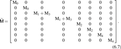
where N is the number of degrees of freedom of the constrained rod. For instance, for the folded structure shown in Figure 4b, N = 10 − 2. In the sequel, we ornament kinetic and kinematic quantities associated with the constrained system with a tilde.
(a) A discrete elastic rod composed of four edges and five nodes and (b) the folded discrete elastic rod obtained by permanently joining two of the edges of the rod together. Color images are available online.
In the event that the rod is in contact with a rough surface, it is prudent not to impose the constraints associated with the contact until the concomitant normal forces have been computed. In the PDER formulation, the contact of a rod with a surface is enforced through the contact of a node. For the purposes of exposition, suppose the kth node is in contact with a stationary planar surface whose unit normal is E2, then we prescribe the constraint forces \documentclass{aastex}\usepackage{amsbsy}\usepackage{amsfonts}\usepackage{amssymb}\usepackage{bm}\usepackage{mathrsfs}\usepackage{pifont}\usepackage{stmaryrd}\usepackage{textcomp}\usepackage{portland, xspace}\usepackage{amsmath, amsxtra}\usepackage{upgreek}\pagestyle{empty}\DeclareMathSizes{10}{9}{7}{6}\begin{document}
$${{\bf F}_{{k_{{ \rm{con}}}}}}$$
\end{document} acting on the node as the sum of a normal force and a friction force:
where vk = \documentclass{aastex}\usepackage{amsbsy}\usepackage{amsfonts}\usepackage{amssymb}\usepackage{bm}\usepackage{mathrsfs}\usepackage{pifont}\usepackage{stmaryrd}\usepackage{textcomp}\usepackage{portland, xspace}\usepackage{amsmath, amsxtra}\usepackage{upgreek}\pagestyle{empty}\DeclareMathSizes{10}{9}{7}{6}\begin{document}
$${ \dot {\bf x}_k}$$
\end{document}. The unit vector is parallel to the slipping direction of the kth node, μs is the coefficient of static friction, and μk is the coefficient of dynamic friction. At the stick-slip transition, vk = 0, the friction force is static, and we prescribe the slip direction to be antiparallel to the direction of the limiting static friction force.
By imposing the integrable constraints, we can also compute the constrained kinetic energy \documentclass{aastex}\usepackage{amsbsy}\usepackage{amsfonts}\usepackage{amssymb}\usepackage{bm}\usepackage{mathrsfs}\usepackage{pifont}\usepackage{stmaryrd}\usepackage{textcomp}\usepackage{portland, xspace}\usepackage{amsmath, amsxtra}\usepackage{upgreek}\pagestyle{empty}\DeclareMathSizes{10}{9}{7}{6}\begin{document}
$$\rm \widetilde T$$
\end{document} of the structure:
where the N × N mass matrix is computed using the 2n × 2n matrix by combining the elements associated with the joined nodes. Similarly, for the elastic potential energy, we need to eliminate several terms associated with bending of the pairs of folded edges. To avoid singularities with the turning angle, it may be necessary to introduce new intrinsic curvature terms into the expression for Ee to arrive at \documentclass{aastex}\usepackage{amsbsy}\usepackage{amsfonts}\usepackage{amssymb}\usepackage{bm}\usepackage{mathrsfs}\usepackage{pifont}\usepackage{stmaryrd}\usepackage{textcomp}\usepackage{portland, xspace}\usepackage{amsmath, amsxtra}\usepackage{upgreek}\pagestyle{empty}\DeclareMathSizes{10}{9}{7}{6}\begin{document}
$$\widetilde{E}_e$$
\end{document}. Related remarks pertain to the potential energy Ua associated with the applied conservative forces. The energies \documentclass{aastex}\usepackage{amsbsy}\usepackage{amsfonts}\usepackage{amssymb}\usepackage{bm}\usepackage{mathrsfs}\usepackage{pifont}\usepackage{stmaryrd}\usepackage{textcomp}\usepackage{portland, xspace}\usepackage{amsmath, amsxtra}\usepackage{upgreek}\pagestyle{empty}\DeclareMathSizes{10}{9}{7}{6}\begin{document}
$$\widetilde{E}_e$$
\end{document} and Ũa are then added to define Ũ. We shall shortly discuss a pair of examples in the Folding a Discrete Elastic Rod section to illustrate these points.
Lagrange's equations of motion for the constrained rod are
\documentclass{aastex}\usepackage{amsbsy}\usepackage{amsfonts}\usepackage{amssymb}\usepackage{bm}\usepackage{mathrsfs}\usepackage{pifont}\usepackage{stmaryrd}\usepackage{textcomp}\usepackage{portland, xspace}\usepackage{amsmath, amsxtra}\usepackage{upgreek}\pagestyle{empty}\DeclareMathSizes{10}{9}{7}{6}\begin{document}
\begin{align*}
\frac { d } { { dt } } \left( { { \frac { \partial \tilde L } { \partial { { \dot \tilde q } ^K } } } } \right) - { \frac { \partial \tilde L } { \partial { { \tilde q } ^K } } } = { \tilde Q_K } , \qquad \left( { K = 1 , \ldots , N } \right) , \tag { 6.4 }
\end{align*}
\end{document}
where \documentclass{aastex}\usepackage{amsbsy}\usepackage{amsfonts}\usepackage{amssymb}\usepackage{bm}\usepackage{mathrsfs}\usepackage{pifont}\usepackage{stmaryrd}\usepackage{textcomp}\usepackage{portland, xspace}\usepackage{amsmath, amsxtra}\usepackage{upgreek}\pagestyle{empty}\DeclareMathSizes{10}{9}{7}{6}\begin{document}
$$\widetilde L$$
\end{document} = \documentclass{aastex}\usepackage{amsbsy}\usepackage{amsfonts}\usepackage{amssymb}\usepackage{bm}\usepackage{mathrsfs}\usepackage{pifont}\usepackage{stmaryrd}\usepackage{textcomp}\usepackage{portland, xspace}\usepackage{amsmath, amsxtra}\usepackage{upgreek}\pagestyle{empty}\DeclareMathSizes{10}{9}{7}{6}\begin{document}
$$\widetilde T$$
\end{document} − \documentclass{aastex}\usepackage{amsbsy}\usepackage{amsfonts}\usepackage{amssymb}\usepackage{bm}\usepackage{mathrsfs}\usepackage{pifont}\usepackage{stmaryrd}\usepackage{textcomp}\usepackage{portland, xspace}\usepackage{amsmath, amsxtra}\usepackage{upgreek}\pagestyle{empty}\DeclareMathSizes{10}{9}{7}{6}\begin{document}
$$\widetilde U$$
\end{document}. Constraint forces \documentclass{aastex}\usepackage{amsbsy}\usepackage{amsfonts}\usepackage{amssymb}\usepackage{bm}\usepackage{mathrsfs}\usepackage{pifont}\usepackage{stmaryrd}\usepackage{textcomp}\usepackage{portland, xspace}\usepackage{amsmath, amsxtra}\usepackage{upgreek}\pagestyle{empty}\DeclareMathSizes{10}{9}{7}{6}\begin{document}
$${{\bf F}_{{{ \rm{c}}_k}}}$$
\end{document} are needed to impose the integrable constraints associated with contact, attachment, or folding. However, in the case where the contact is with a smooth surface, it can be shown that these forces do not contribute to several of the forces K:
Consequently, Equation (6.4) can be integrated using standard methods.
Folding a discrete elastic rod
Imagine modeling a T-shaped structure using a discrete elastic rod. The simplest such model will have four nodes; however, to start the modeling process, we consider a discrete elastic rod with four edges (and five nodes) shown in Figure 4. Imagine constraining the positions of nodes x1 and x3 to be identical, which has the effect of folding the second and third edges onto themselves.*
To establish the equations of motion for the folded structure shown in Figure 4, we need only eight generalized coordinates:
The mass matrix is
The constrained elastic energy \documentclass{aastex}\usepackage{amsbsy}\usepackage{amsfonts}\usepackage{amssymb}\usepackage{bm}\usepackage{mathrsfs}\usepackage{pifont}\usepackage{stmaryrd}\usepackage{textcomp}\usepackage{portland, xspace}\usepackage{amsmath, amsxtra}\usepackage{upgreek}\pagestyle{empty}\DeclareMathSizes{10}{9}{7}{6}\begin{document}
$$\widetilde{E}$$
\end{document} = \documentclass{aastex}\usepackage{amsbsy}\usepackage{amsfonts}\usepackage{amssymb}\usepackage{bm}\usepackage{mathrsfs}\usepackage{pifont}\usepackage{stmaryrd}\usepackage{textcomp}\usepackage{portland, xspace}\usepackage{amsmath, amsxtra}\usepackage{upgreek}\pagestyle{empty}\DeclareMathSizes{10}{9}{7}{6}\begin{document}
$$\widetilde{E}_s$$
\end{document} + \documentclass{aastex}\usepackage{amsbsy}\usepackage{amsfonts}\usepackage{amssymb}\usepackage{bm}\usepackage{mathrsfs}\usepackage{pifont}\usepackage{stmaryrd}\usepackage{textcomp}\usepackage{portland, xspace}\usepackage{amsmath, amsxtra}\usepackage{upgreek}\pagestyle{empty}\DeclareMathSizes{10}{9}{7}{6}\begin{document}
$$\widetilde{E}_b$$
\end{document} can be obtained from Equation (4.2):
The areal moment of inertia in the bending energy expression is defined as
The intrinsic curvature at the T-joint is such that the intrinsic turning angle at this point is 90°. Thus,
\documentclass{aastex}\usepackage{amsbsy}\usepackage{amsfonts}\usepackage{amssymb}\usepackage{bm}\usepackage{mathrsfs}\usepackage{pifont}\usepackage{stmaryrd}\usepackage{textcomp}\usepackage{portland, xspace}\usepackage{amsmath, amsxtra}\usepackage{upgreek}\pagestyle{empty}\DeclareMathSizes{10}{9}{7}{6}\begin{document}
\begin{align*}
{ \bar \kappa _1} = { \bar \kappa _3} = 2. \tag{6.10}
\end{align*}
\end{document}
These modifications to the intrinsic curvatures and bending energies are necessary to avoid singularities associated with turning angles of 180°.
A generalization of this folding procedure used to model a caterpillar-inspired robot is shown in Figures 5 and 6. In this construction, we are modeling the bonding of two segments of a discrete elastic rod by artificially inserting massless freely extensible segments of a rod (i.e., the segment has a Young's modulus of 0). Such a segment is shown as a dashed line in the aforementioned figure. We can then use the folding procedure mentioned earlier to create a discrete elastic rod model for the caterpillar-inspired robot in the A Discrete Model for a Caterpillar-Inspired Soft Robot section.
(a) A discrete elastic rod composed of two segments with eight nodes and a third massless freely extensible segment with a single edge (dashed line). (b) The folded discrete elastic rod obtained by permanently bonding the third edge to the first segment. Color images are available online.
(a) The folded discrete elastic rod from Figure 5 that is obtained by permanently bonding the third edge to the first segment. (b) The folded discrete elastic rod formed by bonding the sixth edge of the first segment to the first edge of the second segment. (c) Introducing intrinsic curvature into the folded rod. Color images are available online.
A Discrete Model for a Single SMA Actuator
A class of soft robots such as those discussed in Refs.2–4 is typically made by assembling a series of actuators composed of nickel-titanium SMA wire enclosed in a flexible casing. We refer to the assembly of wire and flexible casing as an SMA actuator. As electric current is passed through the wire, the wire heats up and transitions from its martensite to the austenite state.33 This transformation bends the actuator and also changes its flexural rigidity. Faithfully simulating the dynamics of a single actuator during this transformation is a necessary precursor to simulating a soft robot assembled from these actuators.
We model the transformation as inducing changes to the intrinsic curvature and flexural rigidity in a rod-based model for the actuator. To obtain an estimate of the material parameters of the SMA actuator during actuation, we consider a single actuator clamped at one end and free at the other under repeated actuation. We first perform an experiment to measure the shape of the hardware actuator over time using automated tracking of high speed video. Next we numerically solve for material parameter values that give the best agreement between the hardware measurements and the results of numerical simulations of the planar DER model. All six of the actuators (which we label #1 through #6) used in the construction of the caterpillar robot were probed in this manner.
We are able to use an optical method based on our earlier work23 to determine the intrinsic curvature of the actuator. The tracking procedure involves three steps. First, given a frame from the video, a colored edge of the actuator is isolated from the rest of the image. Then, a smoothing spline is used to obtain [x(s), y(s)], where s is the arc-length parameter. Using the functions x(s) and y(s), the curvature κ can be computed analytically. A sample of the results for a single actuator is shown in Figure 7. Although the curvature is not uniform along the length of the actuator, we seek to approximate κ in our models using a mean curvature. At each frame, a circle is fit to the outline of the actuator. The mean curvature of the actuator is identified as the inverse of the circle's radius. Paralleling our earlier work with pneu-net actuators,28,34 the mean curvature we find in this manner, after a rescaling and appropriate sign attribution, can be identified with the intrinsic discrete integrated curvature κk used in the PDER model. Representative examples of the time evolution of the mean curvature can be seen in Figure 8a for 10 repeated activation cycles. Every cycle heats the actuator and, without sufficient cooling time, the curvature profile flattens out.
Motion capture data of a cantilevered SMA actuator. (a) Deformed shape of the actuator when an activation pulse signal is applied at t = 0. After a period of ∼2 s, the actuator returns close to its undisturbed state. (b) Measurement of the curvature κ = κ(s, t) of the centerline of the actuator as a function of arc length for various instants of time. Data from t = 0 s to t = 0.5 s are omitted for visual clarity due to the initial high-frequency response of the actuator (cf. Fig. 8a). However, the initial data are readily inferred from the video provided in the Supplementary Data associated with this article. Color images are available online.
PDER simulation of a cantilevered SMA actuator, using 10 nodes with the first 2 fixed. (a) Predicted mean curvature \documentclass{aastex}\usepackage{amsbsy}\usepackage{amsfonts}\usepackage{amssymb}\usepackage{bm}\usepackage{mathrsfs}\usepackage{pifont}\usepackage{stmaryrd}\usepackage{textcomp}\usepackage{portland, xspace}\usepackage{amsmath, amsxtra}\usepackage{upgreek}\pagestyle{empty}\DeclareMathSizes{10}{9}{7}{6}\begin{document}
$$\bar \kappa ( t )$$
\end{document} of the centerline of the actuator over time, overlaying the simulation result with the logistic fit and measured data for actuator #1 over 10 cycles. (b) Deformed shape of the simulated actuator when an activation pulse signal is applied at t = 0. After a period of ∼2 s, the actuator returns close to its undisturbed state. Color images are available online.
The periodic input current (or activation pulse) to the SMA actuator consists of a square pulse, 0.15 s in duration, with a period of 3.54 s. The current changes the curvature of the actuator. Based on a series of tests, a representative sample of which is shown in Figure 8a, we assume that the change in the mean intrinsic curvature follows a logistic curve of the form
\documentclass{aastex}\usepackage{amsbsy}\usepackage{amsfonts}\usepackage{amssymb}\usepackage{bm}\usepackage{mathrsfs}\usepackage{pifont}\usepackage{stmaryrd}\usepackage{textcomp}\usepackage{portland, xspace}\usepackage{amsmath, amsxtra}\usepackage{upgreek}\pagestyle{empty}\DeclareMathSizes{10}{9}{7}{6}\begin{document}
\begin{align*}
\bar \kappa ( t ) = { \bar \kappa _ { { \rm { rest } } } } - A \left( { 1 - \frac { 1 } { { 1 + { e^ { - \frac { { t - { t_0 } } } { \tau } } } } } } \right) , \tag { 7.1 }
\end{align*}
\end{document}
starting from the moment electrical current is applied at t = 0. In this equation, \documentclass{aastex}\usepackage{amsbsy}\usepackage{amsfonts}\usepackage{amssymb}\usepackage{bm}\usepackage{mathrsfs}\usepackage{pifont}\usepackage{stmaryrd}\usepackage{textcomp}\usepackage{portland, xspace}\usepackage{amsmath, amsxtra}\usepackage{upgreek}\pagestyle{empty}\DeclareMathSizes{10}{9}{7}{6}\begin{document}
$${ \bar \kappa _{{ \rm{rest}}}}$$
\end{document} is the resting value of the curvature that it returns to after actuation, A > 0 represents the net decrease in the curvature at the start of actuation, t0 is the time that the curvature is halfway back to its resting value [\documentclass{aastex}\usepackage{amsbsy}\usepackage{amsfonts}\usepackage{amssymb}\usepackage{bm}\usepackage{mathrsfs}\usepackage{pifont}\usepackage{stmaryrd}\usepackage{textcomp}\usepackage{portland, xspace}\usepackage{amsmath, amsxtra}\usepackage{upgreek}\pagestyle{empty}\DeclareMathSizes{10}{9}{7}{6}\begin{document}
$$\bar \kappa ( {t_0} ) = { \bar \kappa _{{ \rm{rest}}}} - A / 2$$
\end{document}], and τ is a time constant. The Matlab function lsqcurvefit is used to solve for the four parameters (\documentclass{aastex}\usepackage{amsbsy}\usepackage{amsfonts}\usepackage{amssymb}\usepackage{bm}\usepackage{mathrsfs}\usepackage{pifont}\usepackage{stmaryrd}\usepackage{textcomp}\usepackage{portland, xspace}\usepackage{amsmath, amsxtra}\usepackage{upgreek}\pagestyle{empty}\DeclareMathSizes{10}{9}{7}{6}\begin{document}
$${ \bar \kappa _{{ \rm{rest}}}}$$
\end{document}, A, τ, t0) that minimize a least-squares error function, \documentclass{aastex}\usepackage{amsbsy}\usepackage{amsfonts}\usepackage{amssymb}\usepackage{bm}\usepackage{mathrsfs}\usepackage{pifont}\usepackage{stmaryrd}\usepackage{textcomp}\usepackage{portland, xspace}\usepackage{amsmath, amsxtra}\usepackage{upgreek}\pagestyle{empty}\DeclareMathSizes{10}{9}{7}{6}\begin{document}
$$\sum { ( \kappa ( t ) - \bar \kappa ( } t , { \bar \kappa _{{ \rm{rest}}}} , A , \tau , {t_0} ) { ) ^2}.$$
\end{document} To prepare the data, we trim the 240 frame-per-second time series data for a given actuator into data for each individual cycle, taking t = 0 to be the instant that the curvature first crosses the threshold κ = −60 m−1 from below. The end of a cycle is chosen as the time when the curvature reaches its minimum value before the next electrical pulse input. As can be seen from Figure 8a, the logistic function in Equation (7.1) qualitatively matches the shape of κ(t) after initial oscillations have died down.
As regards our PDER simulation, we identify κ(t) with the intrinsic curvature \documentclass{aastex}\usepackage{amsbsy}\usepackage{amsfonts}\usepackage{amssymb}\usepackage{bm}\usepackage{mathrsfs}\usepackage{pifont}\usepackage{stmaryrd}\usepackage{textcomp}\usepackage{portland, xspace}\usepackage{amsmath, amsxtra}\usepackage{upgreek}\pagestyle{empty}\DeclareMathSizes{10}{9}{7}{6}\begin{document}
$$\bar \kappa ( t )$$
\end{document} of the rod. The function \documentclass{aastex}\usepackage{amsbsy}\usepackage{amsfonts}\usepackage{amssymb}\usepackage{bm}\usepackage{mathrsfs}\usepackage{pifont}\usepackage{stmaryrd}\usepackage{textcomp}\usepackage{portland, xspace}\usepackage{amsmath, amsxtra}\usepackage{upgreek}\pagestyle{empty}\DeclareMathSizes{10}{9}{7}{6}\begin{document}
$$\bar \kappa ( t )$$
\end{document} is then used to define the reference (or intrinsic) discrete integrated curvatures \documentclass{aastex}\usepackage{amsbsy}\usepackage{amsfonts}\usepackage{amssymb}\usepackage{bm}\usepackage{mathrsfs}\usepackage{pifont}\usepackage{stmaryrd}\usepackage{textcomp}\usepackage{portland, xspace}\usepackage{amsmath, amsxtra}\usepackage{upgreek}\pagestyle{empty}\DeclareMathSizes{10}{9}{7}{6}\begin{document}
$${ \bar \kappa _1} ( t ) , \ldots , { \bar \kappa _{n - 2}} ( t )$$
\end{document} of the nodes of the PDER. In this manner, the SMA actuation is incorporated into the rod model. That is, when the square pulse is activated, the intrinsic curvature changes according to Equation (7.1). Note that the time constant τ can be considered to be a function of the SMA temperature, as seen in Figure 8a for an actuation period of 3.54 s; a longer period of actuation would yield a constant τ but a slower locomotion speed of the caterpillar-inspired soft robot.
For the numerical simulations of the planar DER model, we use the implicit first-order integration scheme suggested in Refs.15,24:
with a time step h = tk+ 1 − tk. At each instant of time tk, we numerically solve the set of nonlinear equations in Equation (7.2) for x(tk+ 1) and \documentclass{aastex}\usepackage{amsbsy}\usepackage{amsfonts}\usepackage{amssymb}\usepackage{bm}\usepackage{mathrsfs}\usepackage{pifont}\usepackage{stmaryrd}\usepackage{textcomp}\usepackage{portland, xspace}\usepackage{amsmath, amsxtra}\usepackage{upgreek}\pagestyle{empty}\DeclareMathSizes{10}{9}{7}{6}\begin{document}
$$\dot {x}$$
\end{document}(tk+ 1) using Matlab's fsolve function. Entries of the force vector F are the sum of forces due to bending, stretching, viscous damping, and frictional ground contact for each node. The actuator is simulated using a discrete elastic rod with n = 10 nodes and a time step of h = 0.001 s. To simulate the boundary conditions at one end of the cantilevered rod, the first two nodes of the discrete elastic rod were fixed.
To estimate the stiffness and damping parameters of the actuator, we consider the oscillations in \documentclass{aastex}\usepackage{amsbsy}\usepackage{amsfonts}\usepackage{amssymb}\usepackage{bm}\usepackage{mathrsfs}\usepackage{pifont}\usepackage{stmaryrd}\usepackage{textcomp}\usepackage{portland, xspace}\usepackage{amsmath, amsxtra}\usepackage{upgreek}\pagestyle{empty}\DeclareMathSizes{10}{9}{7}{6}\begin{document}
$$\bar \kappa ( t )$$
\end{document} during the first 0.4 s of actuation (cf. Fig. 8a). For each of the six actuators and each cycle, the dominant frequency of oscillation is computed using Matlab's periodogram function, and the curvature overshoot is calculated as the minimum value of the measured curvature relative to the logistic curve fit. We use Matlab's nonlinear equation solver fzero to solve for values of the Young's modulus E and viscous damping coefficient δ such that the oscillation frequency and overshoot of the numerical PDER simulation of the actuator most closely match the experimental data. The Young's modulus is presumed to follow the same activation time profile as the intrinsic curvature, assuming that the maximum stiffness is 2.3 times that of the resting stiffness based on the martensitic–austenitic transition of the SMA wire:
\documentclass{aastex}\usepackage{amsbsy}\usepackage{amsfonts}\usepackage{amssymb}\usepackage{bm}\usepackage{mathrsfs}\usepackage{pifont}\usepackage{stmaryrd}\usepackage{textcomp}\usepackage{portland, xspace}\usepackage{amsmath, amsxtra}\usepackage{upgreek}\pagestyle{empty}\DeclareMathSizes{10}{9}{7}{6}\begin{document}
\begin{align*}
E ( t ) = { E_ { { \rm { rest } } } } \left( { 2.3 - { \frac { 1.3 } { 1 + { e^ { - \frac { { t - { t_0 } } } { \tau } } } } } } \right). \tag { 7.3 }
\end{align*}
\end{document}
The damping coefficient δ is assumed to be constant over time. In our simulations, the frequency of oscillation varies strongly with the bending stiffness, while the overshoot and decay time varies more strongly with the damping coefficient.
Best-fit material parameter values for the cantilever SMA actuator are presented in Appendix Table A1, averaged over the 6 actuators and 10 cycles of activation each. Figure 8b shows snapshots of the cantilever DER simulation using average parameter fits from actuator #1. In contrast to the snapshot data shown in Figure 7 where the rod does not have a constant curvature, the simulations in Figure 8b show a rod where each node has the same curvature, based on the mean curvature parameter fit from the experimental data. The temporal behavior of the mean curvature compares favorably to the experimental measurements shown in Figure 7.
A Discrete Model for a Caterpillar-Inspired Soft Robot
The next model we consider is for the caterpillar-inspired soft robot shown in Figure 1. The PDER model for this robot is constructed using a straightforward variation of the folding procedure presented in Folding a Discrete Elastic Rod section (cf. Fig. 5). In this study, we consider a series of ns interconnected PDER segments each containing nn nodes. Each segment can be actuated to vary its intrinsic curvature and stiffness, as in the single-rod example in the previous section. Within a single segment, we label the nodes in order as j = 0, 1, …, nn − 1. The connection from segment k to segment k + 1 is such that the edge connecting nodes nn− 1 and nn− 2 of the kth segment are bonded onto nodes nf and nf + 1 of the (k + 1)th segment, where nf and nb are the number of extra nodes forming forward-facing and rearward-facing foot-like extensions, respectively (cf. Fig. 9a showing the case of nf = 0, nb = 1). The end point of the foot structure will sometimes contact the ground, giving rise to the frictional forces that enable locomotion. In addition, we add a passive spine PDER along the top of the structure that holds the electronics and batteries to power and control the system. The spine rod has one node per segment, such that node j − 1 of the spine is attached to a particular node p of the jth segment.
Locomotion performance of a PDER model for a caterpillar-inspired soft robot. (a) Segment numbering of the model; (b) intrinsic curvature κ0(t) of the segments as a function of time; (c) Young's moduli E(t) of the segments as a function of time; (d) displacement of the front foot of the robot as a function of time; and (e) displacement of the rear foot of the robot as a function of time. The displacements shown in (d, e) are compared to the performance of the fabricated and actuated soft robot (hardware robot). The highest displacement was attained with rear-facing feet configured as shown in (a). Color images are available online.
In our simulations of the caterpillar PDER model, we use the same material parameters for the SMA actuator discussed in A Discrete Model for a Single SMA Actuator section. The parameters for the time series of intrinsic curvature and stiffness of the actuators are taken as the means of the parameters over all measured actuators and actuation cycles. Inputs are based on a gait developed for the experimental prototype shown in Figure 1. For both the hardware robot and the simulation, control inputs are repeated with a period of 3.54 s, with a 1/3 period phase difference between neighboring segments, such that two actuators are activated simultaneously in a wave from the back to the front of the robot. The full list of material parameters for the SMA actuator segments and the passive spine rod is collected in the Appendix.
For our simulations, we use ns = 6 segments with nn = 9 + nf + nb nodes per segment for different combinations of nf, nb = {0, 1}. The spine is attached at node 4 + nf for each segment, and neighboring segments are connected along a single edge, such that nodes nn − 2 − nb and nn − 1 − nb of the kth segment correspond to nodes nf and nf + 1 of the (k + 1)th segment (cf. Fig. 9a).
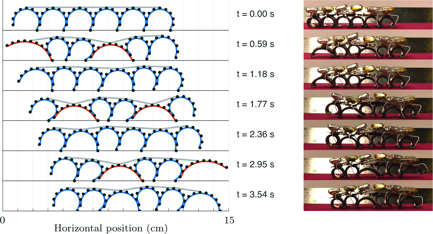
The asymmetry of the foot-like structure (having one additional node below the shared edge on the next rod) appears to be vital for locomotion, based on observations of the physical prototype. In simulation, we investigated a range of different foot shapes, varying the length of the forward and rearward extended foot edges while keeping the total length of each segment constant. The foot shape with maximum horizontal displacement after one complete gait cycle used nf = 0, nb = 1 with the rearward-facing foot edge having length equal to the other edges. The displacement over time for the hardware robot is compared to the simulations in Figure 9, and snapshots of the maximum-displacement simulation are presented with corresponding images of the hardware robot in Figure 10.
Locomotion performance of a caterpillar PDER model compared to a soft robot prototype. Left: snapshots of the model from one full period of the gait cycle. Right: images of the soft robot at corresponding times during a gait cycle. The snapshots are taken from a supplemental video associated with this article. Color images are available online.
The segment actuation that was used to compute the results shown in Figure 7 and the motion of the caterpillar-inspired robot in Figure 10b have been explained in Supplementary Videos S1 and S2.
To compare locomotion performance, we measure the horizontal displacement of the front foot (the last node of the last segment) and back foot (the first node of the first segment). Over a single gait cycle of 3.54 s, the hardware robot has displacement of 36.8 mm (front) and 38.0 mm (back). The best of the simulations has a horizontal displacement of 26.7 mm (front) and 27.0 mm (back). The worst of the simulations has displacement of only 6.9 mm (front) and 8.9 mm (back). Performance for a range of foot shapes is presented in Figure 11. Although our highest displacement simulation based on the material parameters measured in A Discrete Model for a Single SMA Actuator section has on average 28% lower displacement compared to the hardware robot, we are encouraged that the complex PDER model with many parameters is able to qualitatively track the motion of the physical system. Through additional simulations with variations of the parameter values, we find that increasing the stiffness of the actuators by a factor of 20% yields a displacement that is 6.7% greater than the hardware robot, illustrated in Appendix A.6.
Locomotion performance of a caterpillar PDER model with varying foot shapes, measured over a full 3.54 s gait cycle. (a) Heat map of the front foot displacement (mm) and (b) heat map of the rear foot displacement. Forward-foot and rearward-foot extensions are the length of forward-facing foot edges and rearward-facing foot edges, respectively, as a fraction of the length of interior edges. The color scale (in mm) is the same for both plots. Color images are available online.
Our simulations suggest that the locomotion performance is highly sensitive to the geometry of the connections between rods forming the feet that contact the ground, to such an extent that small changes in the foot shape yield simulations with up to a 3.4 times difference in locomotion performance, as shown in Figure 11. Comparisons of the simulation results to video of the hardware prototype reveal a few key differences. At the onset of activation, the hardware appears to generate higher forces than the simulation, causing the caterpillar to leap forward at the start of each step. The shape of the foot end of each segment affects the angle that the end of the rod touches the ground. This observation is significant because forces arising due to change in intrinsic curvature at the first node are normal to the first edge.
The connection of the spine also has a significant effect on the behavior of the system. We investigated other attachment schemes, such as only attaching to the first and last segments, but found that attaching to every segment achieved the best locomotion results. The one-node-per-segment attachment used in the simulation preserves the primary function of the spine, which is to keep the segments from folding over on each other. In the future, the PDER theory may be extended to model rod-on-rod surface contact with frictional and normal forces. Such an extension might provide a more realistic simulation in certain situations.
Conclusions
In this article, we have discussed the application of Bergou et al.'s discrete elastic rod formulation to study and analyze the locomotion of soft robots. The robots of interest are composed of long slender structures that are amenable to modeling using a rod theory. To help facilitate use of the discrete rod formulation, the notion of folding a straight rod is introduced so it can model a soft robot that has a tree-like architecture. This folding strategy was also shown to include a strategy where segments of rods were bonded together. We also showed how recent works on Lagrange's equations of motion for systems of particles can be exploited so as to confidently establish the equations of motion for the discrete rod. Our main goal was to apply the discrete elastic rod formulation to study the difficult problem of developing models for the locomotion of soft robots. A representative example was presented to show the capabilities of the formulation: a caterpillar-inspired soft robot fabricated from SMA actuators in series. The presentation was supplemented by an extensive discussion of parameter estimation and identification. To date, ours is one of the most detailed analysis of locomoting soft robots in the literature. It is straightforward to consider modeling other locomoting soft robots using this formulation, and we hope this article inspires the soft robotics community to explore the development of models of this type.
Footnotes
Acknowledgments
This research was partially supported by grant numbers W911NF-16-1-0148 (to CMU), W911NF-16-1-0242 (to UCB), and W911NF-16-1-0244 (to UMD) from the U.S. Army Research Organization. These grants are administered by Dr. Samuel C. Stanton. The work of N.N.G. was supported by a Berkeley Fellowship awarded by the University of California, Berkeley and a National Defense Science and Engineering Graduate Fellowship. The authors are grateful to three anonymous reviewers for their extensive constructive critiques of an earlier draft of this article.
Author Disclosure Statement
No competing financial interests exist.
Supplementary Material
Appendix A. A Shape Memory Alloy Actuator Fabrication and Characterization
This appendix discusses the fabrication and characterization of the shape memory alloy (SMA) actuators that are modeled in this article. The actuators were developed at the Soft Materials Laboratory (SML) at Carnegie Mellon University (CMU).A1
References
1.
GallowayKC, BeckerKP, PhillipsB, et al.Soft robotic grippers for biological sampling on deep reefs. Soft Robotics, 2016; 3:23–33.
2.
LaschiC, CianchettiM, MazzolaiB, et al.Soft robot arm inspired by the octopus. Adv Robotics, 2012; 26:709–727.
3.
SeokS, OnalCD, ChoKJ, et al.Meshworm: A peristaltic soft robot with antagonistic nickel titanium coil actuators. IEEE/ASME Trans Mech, 2013; 18:1485–1497.
4.
LinHT, LeiskGG, TrimmerBA. Goqbot: A caterpillar-inspired soft-bodied rolling robot. Bioinspir Biomim, 2011; 6:026-007.
5.
ChenevierJ, GonzálezD, AguadoJV, et al.Reduced-order modeling of soft robots. PLoS One, 2018; 13:1–15.
6.
DuriezC. Control of elastic soft robots based on real-time finite element method. In: 2013 IEEE International Conference on Robotics and Automation. Milpitas, CA: IEEE, 2013 pp. 3982–3987.
7.
DuriezC, BiezeT. Soft robot modeling, simulation and control in real-time (Soft Robotics: Trends, Applications and Challenges, vol. 17) In: Laschi C, Rossiter J, Iida F, Cianchetti M, Margheri L. (Eds). Cham, Switzerland: Springer, 2017 pp. 103–109.
8.
GraziosoS, Di GironimoG, SicilianoB. A geometrically exact model for soft continuum robots: The finite element deformation space formulation. Soft Robotics 2019. DOI: https://doi.org/10.1089/soro.2018.0047.
9.
LipsonH.Challenges and opportunities for design, simulation, and fabrication of soft robots. Soft Robotics, 2014; 1:21–27.
10.
RendaF, Giorgio-SerchiF, BoyerF, et al.Senevuratne: A unified multi-soft-body dynamic model for underwater soft robots. Int J Rob Res, 2018; 37:648–666.
11.
RungeG, RaatzG. A framework for the automated design and modelling of soft robotic systems. CIRP Ann, 2017; 66:9–12.
12.
ZhouX, MajidiC, O'ReillyOM. Flexing into motion: A locomotion mechanism for soft robots. Int J Nonlin Mech, 2015; 74:7–17.
13.
ZhouX, MajidiC, O'ReillyOM. Soft hands: an analysis of some gripping mechanisms in soft robot design. Int J Solids Struct, 2015; 64–65:155–165.
14.
AudolyB, ClauvelinN, BrunPT, et al.A discrete geometric approach for simulating the dynamics of thin viscous threads. J Comput Phys, 2013; 253:18–49.
15.
BergouM, AudolyB, VougaE, et al.Discrete viscous threads. ACM Trans Graph, 2010; 29:116:1–116:10.
16.
BergouM, WardetzkyM, RobinsonS, et al.Discrete elastic rods. ACM Trans Graph, 2008; 27:63:1–63:12.
17.
LinnJ, DreßlerK. Discrete Cosserat rod models based on the difference geometry of framed curves for interactive simulation of flexible cables (Math for the Digital Factory, Mathematics in Industry, vol. 27) In: Ghezzi L, Hömberg D, Landry C. (Eds). Cham, Switzerland: Springer International Publishing AG, 2017, pp. 289–319.
18.
LoockA, SchömerE, StadtwaldI. A virtual environment for interactive assembly simulation: From rigid bodies to deformable cables. In: 5th World Multiconference on Systemics, Cybernetics and Informatics. Winter Garden, FL: International Institute of Informatics and Systemics, 2001, pp. 325–332.
19.
LvN, LiuJ, DingX, et al.Physically based real-time interactive assembly simulation of cable harness. J Manuf Syst, 2017; 43(Pt 3):385–399 [Special Issue on the 12th International Conference on Frontiers of Design and Manufacturing].
20.
CaseyJ.Geometrical derivation of Lagrange's equations for a system of particles. Am J Phys, 1994; 62:836–847.
21.
O'ReillyOM.Intermediate Engineering Dynamics: A Unified Treatment of Newton-Euler and Lagrangian Mechanics. Cambridge: Cambridge University Press, 2008.
22.
ZhouX, MajidiC, O'ReillyOM. Energy efficiency in friction-based locomotion mechanisms for soft and hard robots: Slower can be faster. Nonlin Dyn, 2014; 78:2811–2821.
23.
Daily-DiamondCA, NoveliaA, O'ReillyOM. Dynamical analysis and development of a biologically inspired SMA caterpillar robot. Bioinspir Biomim, 2017; 12:056-005.
24.
JawedMK, NoveliaA, O'ReillyOM. A Primer on the Kinematics of Discrete Elastic Rods. SpringerBriefs. in Applied Sciences and Technology. New York: Springer-Verlag, 2018.
25.
O'ReillyOM, SrinivasaAR. A simple treatment of constraint forces and constraint moments in the dynamics of rigid bodies. ASME Appl Mech Rev, 2014; 67:014.801–014.808.
26.
TrimmerBA, IssbernerJ. Kinematics of soft-bodied, legged locomotion in Manduca sexta larvae. Biol Bull, 2007; 212:130–142.
27.
BukowickiM, Ekiel-JeżewskaML. Different bending models predict different dynamics of sedimenting elastic trumbbells. Soft Matter, 2018; 1–16. DOI: https://dx-doi-org.web.bisu.edu.cn/10.1039/C8SM00604K.
28.
de PayrebruneKM, O'ReillyOM. On constitutive relations for a rod-based model of a pneu-net bending actuator. Extreme Mech Lett, 2016; 8:38–46.
29.
SyngeJL, GriffithBA. Principles of Mechanics, 3rd ed. New York: McGraw-Hill, 1959.
30.
ConnellyR, DemaineED, RoteG. Straightening polygonal arcs and convexifying polygonal cycles. In: Proceedings of the 41st Annual Symposium on Foundations of Computer Science. Long Beach, CA: IEEE, 2000, pp. 432–442.
31.
DemaineED, O'RourkeJ. A survey of folding and unfolding in computational geometry (Combinatorial and Computational Geometry, Mathematical Sciences Research Institute Publications, vol. 52) In: Goodman JE, Pach J, Welzl E. (Eds). New York: Cambridge University Press, 2005, pp. 167–211.
SeeleckeS, MullerI. Shape memory alloy actuators in smart structures: Modeling and simulation. Appl Mech Rev, 2004; 57:23–46.
34.
de PayrebruneKM, O'ReillyOM. On the development of rod-based models for pneumatically actuated soft robot actuators a five-parameter constitutive relation. Int. J Solids Struct, 2017; 120:226–235.
Supplementary Material
Please find the following supplemental material available below.
For Open Access articles published under a Creative Commons License, all supplemental material carries the same license as the article it is associated with.
For non-Open Access articles published, all supplemental material carries a non-exclusive license, and permission requests for re-use of supplemental material or any part of supplemental material shall be sent directly to the copyright owner as specified in the copyright notice associated with the article.


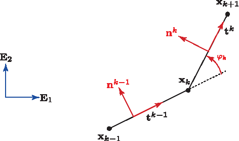


 (cf.
27
and references therein).
(cf.
27
and references therein).


 denotes the length of the ith edge in the reference configuration. If the rod is not homogeneous or of a uniform cross-section, then Mi must be computed using a more primitive prescription:


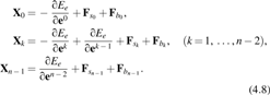


 are
are
 :
:


 is parallel to the slipping direction of the kth node, μs is the coefficient of static friction, and μk is the coefficient of dynamic friction. At the stick-slip transition,
 is computed using the 2n × 2n matrix
  by combining the elements associated with the joined nodes. Similarly, for the elastic potential energy, we need to eliminate several terms associated with bending of the pairs of folded edges. To avoid singularities with the turning angle, it may be necessary to introduce new intrinsic curvature terms into the expression for Ee to arrive at
  K
:
K
:

 is
is