Closed-Loop Control Through Self-Sensing of a Joule-Heated Twisted and Coiled Polymer Muscle

Abstract

The twisted and coiled polymer muscle (TCPM) has two major benefits: low weight and low cost. Therefore, this new type of actuator is increasingly used in robotic applications where these benefits are relevant. Closed-loop control of these muscles, however, requires additional sensors that add weight and cost, negating the muscles' intrinsic benefits. Self-sensing enables feedback without added sensors. In this article, we investigate the feasibility of using self-sensing in closed-loop control of a Joule-heated muscle. We use a hardware module that is capable of driving the muscle, and simultaneously providing sensor measurements based on inductance. A mathematical model relates the measurements to the deflection. In combination with a simple force model, we can estimate both deflection and force, and control either of them. For a muscle that operates within deflections of [10, 30] mm and forces of [0.32, 0.51] N, our self-sensing method exhibited a 95% confidence interval of 2.14 mm around a mean estimation error of −0.27 mm and 29.0 mN around a mean estimation error of 7.5 mN, for the estimation of, respectively, deflection and force. We conclude that self-sensing in closed-loop control of Joule-heated TCPMs is feasible and may facilitate further deployment of such actuators in applications where low cost and weight are critical.

Introduction

The recently developed actuation principle represented by the twisted and coiled polymer muscle (TCPM) has a number of benefits that make it interesting for application in soft robotics.¹ Two major benefits are its low weight and low cost. The working principle of this actuator is based on the thermal torsion effect.² Twisting a fiber with a substructure highly aligned in the direction of the fiber, such as polymer chains or carbon nanotubes, results in a helically aligned substructure. Radial expansion of the twisted fiber and entropic contraction of the helical substructure generate a torque in the opposite direction of the twist. In nylon, both effects can be induced through heating. These torsional actuators become linear actuators through coiling.^2,3

Of the varieties of the TCPM, the thermally activated Joule-heated nylon muscle receives the most attention. This specific type already has a wide range of applications: robotic fingers,^4–6 joints,^7–9 orthoses,^10,11 complete robots,^12,13 or being embedded in a silicon manipulator,¹⁴ silicon skin for robotic facial expressions,¹⁵ or a self-adjusting sports bra.¹⁶

Systems that benefit most from TCPMs are typically lightweight and inexpensive, and they should function in versatile environments. However, most TCPM control schemes rely either on added sensors to enable feedback control^{4–7,17–20} or on predictable circumstances to enable feedforward control.²¹ Added sensors increase weight and cost, negating two major benefits of these actuators. Accurate feedforward control requires a controlled environment, which limits its usability in real-life applications. One way to enjoy the benefits of TCPMs without the drawbacks of added sensors or complex models is through self-sensing. This means that a system determines its state through the interpretation of input-signal behavior, use of special input signals, or connecting additional electrical leads to existing hardware.²² Self-sensing in TCPMs will provide an inexpensive and light-weight way to implement feedback.

TCPMs with Joule heating possess self-sensing capabilities, as demonstrated in our previous work.²³ We show the potential to use both resistance and inductance of heating wires for self-sensing purposes. Next to our work, three studies on sensing in TCPMs focus on modeling the resistance of coated nylon muscles.^24–26 Two of these works use auto-coiled muscles.^24,25 The first work contributes a phenomenological approach to derive a sensing model.²⁴ It relates resistance of a coated fiber to geometric changes during stretching of the coil. However, this approach does not include actuation, and it therefore cannot be applied as a self-sensing model. The second work contributes an analysis of the resistance when actuating the muscle.²⁵ The authors found nonlinearities in the resistance attributed to coil windings making contact with each other. The third study uses mandrel-coiled muscles embedded in a silicon manipulator.²⁶ The authors use the muscles purely as sensors, instead of actuators, and propose a fourth-order polynomial fit as a measurement model. Although these contributions demonstrate the capability for self-sensing, none use self-sensing to close the feedback loop.

In this article, we close the feedback loop via self-sensing. We first identify and validate parameters for two models: one model to estimate deflection via the muscle's inductance, and another model to estimate force, whereby the model inputs are power and estimated deflection. Second, with the models applied, we implement a feedback loop through self-sensing, and perform simple control tasks, as illustrated by Figure 1.

FIG. 1.

Impression of a self-sensing muscle. A control signal P is used to both drive the muscle to generate the force F and measure the inductance L of the Joule-heating wire. Based on the measurement and the previous control input, the self-sensing and control module estimates the force \documentclass{aastex}\usepackage{amsbsy}\usepackage{amsfonts}\usepackage{amssymb}\usepackage{bm}\usepackage{mathrsfs}\usepackage{pifont}\usepackage{stmaryrd}\usepackage{textcomp}\usepackage{portland, xspace}\usepackage{amsmath, amsxtra}\usepackage{upgreek}\pagestyle{empty}\DeclareMathSizes{10}{9}{7}{6}\begin{document} $$\hat F$$ \end{document} and deflection \documentclass{aastex}\usepackage{amsbsy}\usepackage{amsfonts}\usepackage{amssymb}\usepackage{bm}\usepackage{mathrsfs}\usepackage{pifont}\usepackage{stmaryrd}\usepackage{textcomp}\usepackage{portland, xspace}\usepackage{amsmath, amsxtra}\usepackage{upgreek}\pagestyle{empty}\DeclareMathSizes{10}{9}{7}{6}\begin{document} $$\hat x$$ \end{document} , and it, subsequently, determines the new control signal. Color images are available online.

We start with an explanation of the methods. The subsequent section contains the experimental validation of our methods. Next, we present the results of the experiments. Finally, we discuss our work and provide conclusions.

Self-Sensing and Control Methods

We first describe the hardware that combines actuation and sensing. Next, we introduce the models used for self-sensing of deflection and estimation of force, as well as their online implementations. Finally, we introduce the control method.

Combined actuation and sensing

Although several ways exist to activate the TCPM, we choose Joule heating by means of a constantan resistance wire. Joule heating has the benefit that it can be used for self-sensing.²³ In this article, we make use of hardware that realizes this principle.²⁷ The so-called Muscle Drive (MD) drives the TCPM by applying a Pulse Width Modulated (PWM) signal with a controlled duty cycle D. The electrical response of the TCPM during the off time of a signal period relates to inductance. Based on this response, the MD determines a measure of inductance L called decay time.²⁷

Self-sensing model

In our previous work, we introduced a self-sensing model to estimate deflection x, force F, and temperature, when measuring both inductance and resistance.²³ In this article, we first use the actuation power P to estimate the contribution of temperature to force F_T. Next, we use L to determine x and velocity \documentclass{aastex}\usepackage{amsbsy}\usepackage{amsfonts}\usepackage{amssymb}\usepackage{bm}\usepackage{mathrsfs}\usepackage{pifont}\usepackage{stmaryrd}\usepackage{textcomp}\usepackage{portland, xspace}\usepackage{amsmath, amsxtra}\usepackage{upgreek}\pagestyle{empty}\DeclareMathSizes{10}{9}{7}{6}\begin{document} $$\dot {x}$$ \end{document} . We calculate their contribution to force F_l via a mechanical model. Addition of F_T, F_l, and a force offset F_o gives the total force. Figure 2 illustrates this process. Note that the symbol L in this article does not represent physical inductance, but an assumed proportionally related measure thereof.

FIG. 2.

Block diagram for estimation and control. The gray dashed rectangle contains the functionality of the Muscle Drive (MD). Within the MD, the switch indicates that either the deflection estimate \documentclass{aastex}\usepackage{amsbsy}\usepackage{amsfonts}\usepackage{amssymb}\usepackage{bm}\usepackage{mathrsfs}\usepackage{pifont}\usepackage{stmaryrd}\usepackage{textcomp}\usepackage{portland, xspace}\usepackage{amsmath, amsxtra}\usepackage{upgreek}\pagestyle{empty}\DeclareMathSizes{10}{9}{7}{6}\begin{document} $$\hat x$$ \end{document} or the force estimate \documentclass{aastex}\usepackage{amsbsy}\usepackage{amsfonts}\usepackage{amssymb}\usepackage{bm}\usepackage{mathrsfs}\usepackage{pifont}\usepackage{stmaryrd}\usepackage{textcomp}\usepackage{portland, xspace}\usepackage{amsmath, amsxtra}\usepackage{upgreek}\pagestyle{empty}\DeclareMathSizes{10}{9}{7}{6}\begin{document} $$\hat F$$ \end{document} is used as input for the controller, alongside reference r, resulting in either control of deflection x or force F. The Universal Testing Machine (UTM) acts as a load on the muscle. When the MD controls force, the UTM imposes deflection, and vice versa. The temperature model uses power input P to compute the contribution of temperature to force \documentclass{aastex}\usepackage{amsbsy}\usepackage{amsfonts}\usepackage{amssymb}\usepackage{bm}\usepackage{mathrsfs}\usepackage{pifont}\usepackage{stmaryrd}\usepackage{textcomp}\usepackage{portland, xspace}\usepackage{amsmath, amsxtra}\usepackage{upgreek}\pagestyle{empty}\DeclareMathSizes{10}{9}{7}{6}\begin{document} $${ \hat F_T}$$ \end{document} , as in Equation (1). The deflection and velocity estimator represents the measurement of deflection based on decay time L in Equation (4), the subsequent low-pass filtering of the deflection measurement, and taking the backward difference to find velocity \documentclass{aastex}\usepackage{amsbsy}\usepackage{amsfonts}\usepackage{amssymb}\usepackage{bm}\usepackage{mathrsfs}\usepackage{pifont}\usepackage{stmaryrd}\usepackage{textcomp}\usepackage{portland, xspace}\usepackage{amsmath, amsxtra}\usepackage{upgreek}\pagestyle{empty}\DeclareMathSizes{10}{9}{7}{6}\begin{document} $$\hat \dot x$$ \end{document} . The Standard Linear Solid model calculates the contribution \documentclass{aastex}\usepackage{amsbsy}\usepackage{amsfonts}\usepackage{amssymb}\usepackage{bm}\usepackage{mathrsfs}\usepackage{pifont}\usepackage{stmaryrd}\usepackage{textcomp}\usepackage{portland, xspace}\usepackage{amsmath, amsxtra}\usepackage{upgreek}\pagestyle{empty}\DeclareMathSizes{10}{9}{7}{6}\begin{document} $${ \hat F_l}$$ \end{document} to force by deflection and velocity by using Equation (6). The total force estimate \documentclass{aastex}\usepackage{amsbsy}\usepackage{amsfonts}\usepackage{amssymb}\usepackage{bm}\usepackage{mathrsfs}\usepackage{pifont}\usepackage{stmaryrd}\usepackage{textcomp}\usepackage{portland, xspace}\usepackage{amsmath, amsxtra}\usepackage{upgreek}\pagestyle{empty}\DeclareMathSizes{10}{9}{7}{6}\begin{document} $$\hat F$$ \end{document} is found by adding \documentclass{aastex}\usepackage{amsbsy}\usepackage{amsfonts}\usepackage{amssymb}\usepackage{bm}\usepackage{mathrsfs}\usepackage{pifont}\usepackage{stmaryrd}\usepackage{textcomp}\usepackage{portland, xspace}\usepackage{amsmath, amsxtra}\usepackage{upgreek}\pagestyle{empty}\DeclareMathSizes{10}{9}{7}{6}\begin{document} $${ \hat F_l} , \;{ \hat F_T}$$ \end{document} , and force offset F_o. Finally, the PID controller with anti-windup determines the control signal by using Equation (7).

For the estimation of F_T, we disregard the heating time of the resistance wire and assume it heats the fiber homogeneously. We do not measure temperature independently, and we want to use a minimal set of fitted parameters. Therefore, rather than using temperature, we directly relate input power P to the contribution of temperature to force F_T. A first-order model describes the relationship between P, F_T and its derivative with respect to time \documentclass{aastex}\usepackage{amsbsy}\usepackage{amsfonts}\usepackage{amssymb}\usepackage{bm}\usepackage{mathrsfs}\usepackage{pifont}\usepackage{stmaryrd}\usepackage{textcomp}\usepackage{portland, xspace}\usepackage{amsmath, amsxtra}\usepackage{upgreek}\pagestyle{empty}\DeclareMathSizes{10}{9}{7}{6}\begin{document} $$\dot {F}_T$$ \end{document} as a function of time t: \documentclass{aastex}\usepackage{amsbsy}\usepackage{amsfonts}\usepackage{amssymb}\usepackage{bm}\usepackage{mathrsfs}\usepackage{pifont}\usepackage{stmaryrd}\usepackage{textcomp}\usepackage{portland, xspace}\usepackage{amsmath, amsxtra}\usepackage{upgreek}\pagestyle{empty}\DeclareMathSizes{10}{9}{7}{6}\begin{document} \begin{align*} { \dot F_T} ( t ) = { \kappa _P}P ( t ) - { \kappa _c}{F_T} ( t ) { \rm{ , }} \tag{1} \end{align*} \end{document}

where κ_P and κ_c represent the coefficient of conductive heating and convective cooling, respectively. Since F_T represents the contribution of temperature to force, κ_P includes a factor modeling the influence of temperature on force and a factor to correct for power dissipated by the wire directly to the air. We find P by: \documentclass{aastex}\usepackage{amsbsy}\usepackage{amsfonts}\usepackage{amssymb}\usepackage{bm}\usepackage{mathrsfs}\usepackage{pifont}\usepackage{stmaryrd}\usepackage{textcomp}\usepackage{portland, xspace}\usepackage{amsmath, amsxtra}\usepackage{upgreek}\pagestyle{empty}\DeclareMathSizes{10}{9}{7}{6}\begin{document} \begin{align*} P ( t ) = D { ( t ) ^2 } { R_ { \rm { m } } } { \left( { { \frac { { U_ { \rm { b } } } } { { R_ { \rm { b } } } } } } \right) ^2 } { \rm { , } } \tag { 2 } \end{align*} \end{document}

where U_b is the voltage at the connectors of the drive when \documentclass{aastex}\usepackage{amsbsy}\usepackage{amsfonts}\usepackage{amssymb}\usepackage{bm}\usepackage{mathrsfs}\usepackage{pifont}\usepackage{stmaryrd}\usepackage{textcomp}\usepackage{portland, xspace}\usepackage{amsmath, amsxtra}\usepackage{upgreek}\pagestyle{empty}\DeclareMathSizes{10}{9}{7}{6}\begin{document} $$D = 1$$ \end{document} , R_b is the electrical resistance of the circuit as measured at the connectors, and R_m is the electrical resistance of the Joule-heating part of the circuit. Note that we neglect the influence of reactive power on heating of the muscle. The muscles used in this article have an inductance in the order of magnitude of 1 μH. With a signal frequency in the order of magnitude of 100 Hz, the reactive power is around 0.01% of the total power.

The model for computing deflection is taken directly from our previous work.²³ It relates L to x and temperature T by: \documentclass{aastex}\usepackage{amsbsy}\usepackage{amsfonts}\usepackage{amssymb}\usepackage{bm}\usepackage{mathrsfs}\usepackage{pifont}\usepackage{stmaryrd}\usepackage{textcomp}\usepackage{portland, xspace}\usepackage{amsmath, amsxtra}\usepackage{upgreek}\pagestyle{empty}\DeclareMathSizes{10}{9}{7}{6}\begin{document} \begin{align*} L ( t ) = { \frac { { \lambda _x } } { x ( t ) + { \lambda _l } } } + { \lambda _T } T ( t ) + { \lambda _o } { \rm { , } } \tag { 3 } \end{align*} \end{document}

with λ_x, λ_l, λ_T, and λ_o as fitted parameters. In contrast to our previous work,²³ we use a constantan resistance wire that exhibits almost constant resistance regardless of temperature. We can therefore neglect the influence of temperature on the actuation and measurement signal. We further neglect the potential influences of temperature on inductance that do not also influence deflection. Omitting temperature from Equation (3) and rewriting the equation to act as a self-sensing model results in: \documentclass{aastex}\usepackage{amsbsy}\usepackage{amsfonts}\usepackage{amssymb}\usepackage{bm}\usepackage{mathrsfs}\usepackage{pifont}\usepackage{stmaryrd}\usepackage{textcomp}\usepackage{portland, xspace}\usepackage{amsmath, amsxtra}\usepackage{upgreek}\pagestyle{empty}\DeclareMathSizes{10}{9}{7}{6}\begin{document} \begin{align*} x ( t ) = { \frac { { \lambda _x } - { \lambda _l } ( L ( t ) - { \lambda _o } ) } { L ( t ) - { \lambda _o } } } . \tag { 4 } \end{align*} \end{document}

As a force model we combine the Standard Linear Solid (SLS) model for the mechanical behavior,²⁸ with a contribution by temperature in parallel, as shown in Figure 3. This makes the force model:

\documentclass{aastex}\usepackage{amsbsy}\usepackage{amsfonts}\usepackage{amssymb}\usepackage{bm}\usepackage{mathrsfs}\usepackage{pifont}\usepackage{stmaryrd}\usepackage{textcomp}\usepackage{portland, xspace}\usepackage{amsmath, amsxtra}\usepackage{upgreek}\pagestyle{empty}\DeclareMathSizes{10}{9}{7}{6}\begin{document} \begin{align*} F ( t ) = {F_l} ( t ) + {F_T} ( t ) + {F_{ \rm{o}}}{ \rm{ , }} \tag{5} \end{align*} \end{document}

in which F_o represents a force offset, and for which the contribution by F_l is governed by: \documentclass{aastex}\usepackage{amsbsy}\usepackage{amsfonts}\usepackage{amssymb}\usepackage{bm}\usepackage{mathrsfs}\usepackage{pifont}\usepackage{stmaryrd}\usepackage{textcomp}\usepackage{portland, xspace}\usepackage{amsmath, amsxtra}\usepackage{upgreek}\pagestyle{empty}\DeclareMathSizes{10}{9}{7}{6}\begin{document} \begin{align*} { { \dot F } _l } \, ( t ) = - \frac { { { k_2 } } } { c } { F_l } \, ( t ) + \frac { { { k_1 } { k_2 } } } { c } x \, ( t ) + ( { k_1 } + { k_2 } ) \, \dot x \, ( t ) { \rm { , } } \tag { 6 } \end{align*} \end{document}

with stiffnesses k₁ and k₂, and damping c. These three parameters, in addition to F_o, are fitted parameters.

FIG. 3.

Representation of the force model used for the muscles: the Standard Linear Solid model,²⁸ with a contribution by temperature in parallel.

Estimator implementation

F_T and F_l can be found by transferring their respective models to discrete time. However, filtering is required to process deflection measurements into usable estimates, and we need to estimate \documentclass{aastex}\usepackage{amsbsy}\usepackage{amsfonts}\usepackage{amssymb}\usepackage{bm}\usepackage{mathrsfs}\usepackage{pifont}\usepackage{stmaryrd}\usepackage{textcomp}\usepackage{portland, xspace}\usepackage{amsmath, amsxtra}\usepackage{upgreek}\pagestyle{empty}\DeclareMathSizes{10}{9}{7}{6}\begin{document} $$\dot {x}$$ \end{document} as an input for the force model. To that end, we apply a low-pass filter, with a cut-off frequency at 1/9 Hz. Subsequently, we find the velocity by taking the backward difference of the deflection estimate.

Control design

To keep control simple, we choose to use proportional-integral-derivative (PID) control with anti-windup via back calculation to deal with the actuation-signal limits.²⁹ The control law to find the desired actuation signal \documentclass{aastex}\usepackage{amsbsy}\usepackage{amsfonts}\usepackage{amssymb}\usepackage{bm}\usepackage{mathrsfs}\usepackage{pifont}\usepackage{stmaryrd}\usepackage{textcomp}\usepackage{portland, xspace}\usepackage{amsmath, amsxtra}\usepackage{upgreek}\pagestyle{empty}\DeclareMathSizes{10}{9}{7}{6}\begin{document} $${P_{ \rm{d}}}$$ \end{document} is given by:

with the error e and ė its derivative with respect to time. Control parameters K_p, T_d, and T_i represent the proportional gain, and the derivative and integral time constants, respectively. We saturate \documentclass{aastex}\usepackage{amsbsy}\usepackage{amsfonts}\usepackage{amssymb}\usepackage{bm}\usepackage{mathrsfs}\usepackage{pifont}\usepackage{stmaryrd}\usepackage{textcomp}\usepackage{portland, xspace}\usepackage{amsmath, amsxtra}\usepackage{upgreek}\pagestyle{empty}\DeclareMathSizes{10}{9}{7}{6}\begin{document} $${P_{ \rm{d}}}$$ \end{document} by using: \documentclass{aastex}\usepackage{amsbsy}\usepackage{amsfonts}\usepackage{amssymb}\usepackage{bm}\usepackage{mathrsfs}\usepackage{pifont}\usepackage{stmaryrd}\usepackage{textcomp}\usepackage{portland, xspace}\usepackage{amsmath, amsxtra}\usepackage{upgreek}\pagestyle{empty}\DeclareMathSizes{10}{9}{7}{6}\begin{document} \begin{align*} P ( t ) = \max \, ( {P_{{ \rm{min}}}} , \min \, ( {P_{{ \rm{max}}}} , {P_{ \rm{d}}} ( t ) ) ) \tag{9} \end{align*} \end{document}

with \documentclass{aastex}\usepackage{amsbsy}\usepackage{amsfonts}\usepackage{amssymb}\usepackage{bm}\usepackage{mathrsfs}\usepackage{pifont}\usepackage{stmaryrd}\usepackage{textcomp}\usepackage{portland, xspace}\usepackage{amsmath, amsxtra}\usepackage{upgreek}\pagestyle{empty}\DeclareMathSizes{10}{9}{7}{6}\begin{document} $${P_{{ \rm{max}}}}$$ \end{document} and \documentclass{aastex}\usepackage{amsbsy}\usepackage{amsfonts}\usepackage{amssymb}\usepackage{bm}\usepackage{mathrsfs}\usepackage{pifont}\usepackage{stmaryrd}\usepackage{textcomp}\usepackage{portland, xspace}\usepackage{amsmath, amsxtra}\usepackage{upgreek}\pagestyle{empty}\DeclareMathSizes{10}{9}{7}{6}\begin{document} $${P_{{ \rm{min}}}}$$ \end{document} representing the respective upper and lower bound of the actuation signal. We use this control law for both deflection control and force control. Therefore, the reference r can be either a deflection or a force, and we use the corresponding estimate, \documentclass{aastex}\usepackage{amsbsy}\usepackage{amsfonts}\usepackage{amssymb}\usepackage{bm}\usepackage{mathrsfs}\usepackage{pifont}\usepackage{stmaryrd}\usepackage{textcomp}\usepackage{portland, xspace}\usepackage{amsmath, amsxtra}\usepackage{upgreek}\pagestyle{empty}\DeclareMathSizes{10}{9}{7}{6}\begin{document} $$\hat x$$ \end{document} or \documentclass{aastex}\usepackage{amsbsy}\usepackage{amsfonts}\usepackage{amssymb}\usepackage{bm}\usepackage{mathrsfs}\usepackage{pifont}\usepackage{stmaryrd}\usepackage{textcomp}\usepackage{portland, xspace}\usepackage{amsmath, amsxtra}\usepackage{upgreek}\pagestyle{empty}\DeclareMathSizes{10}{9}{7}{6}\begin{document} $$\hat F$$ \end{document} , to calculate e and ė. We discretize the integral action by using Euler's method.

Stability analysis

Stability analysis requires knowledge of the full system: the physical actuator, its controller, and the load. However, for the method in this article we do not make assumptions regarding the behavior of the load. In other words, we do not know the behavior of the blocks representing the Universal Testing Machine (UTM) and the physical muscle in Figure 2 for arbitrary cases. This means that we cannot analyze stability for the full system. However, we can analyze the stability of the control loop within the gray dotted lines representing the MD, by assuming a constant x, and hence a constant L. This case represents force control with a constant deflection. In this case, closed-loop control is reduced to the interaction between the temperature model in Equation (1) and the control law in Equation (7). A potential source of instability is the saturation in Equation (9). Separating the nonlinearity from the dynamics allows for stability analysis via describing functions.³⁰ To that end, we determine the transfer function from P to \documentclass{aastex}\usepackage{amsbsy}\usepackage{amsfonts}\usepackage{amssymb}\usepackage{bm}\usepackage{mathrsfs}\usepackage{pifont}\usepackage{stmaryrd}\usepackage{textcomp}\usepackage{portland, xspace}\usepackage{amsmath, amsxtra}\usepackage{upgreek}\pagestyle{empty}\DeclareMathSizes{10}{9}{7}{6}\begin{document} $${P_{ \rm{d}}}$$ \end{document} , and we use a describing function to represent the saturation in the controller. In the Laplace domain, the transfer function that represents the interaction between Equations (1) and (7) is given by: \documentclass{aastex}\usepackage{amsbsy}\usepackage{amsfonts}\usepackage{amssymb}\usepackage{bm}\usepackage{mathrsfs}\usepackage{pifont}\usepackage{stmaryrd}\usepackage{textcomp}\usepackage{portland, xspace}\usepackage{amsmath, amsxtra}\usepackage{upgreek}\pagestyle{empty}\DeclareMathSizes{10}{9}{7}{6}\begin{document} \begin{align*} \frac { { { P_ { \rm { d } } } } } { P } = { \frac { - { K_ { \rm { p } } } { T_ { \rm { d } } } { \kappa _P } { s^2 } + \left( { \frac { 1 } { { { T_i } } } - { \kappa _P } { K_ { \rm { p } } } } \right) s + \left( { { \frac { { \kappa _c } } { { T_i } } } - { \frac { { \kappa _P } { K_ { \rm { p } } } } { { T_i } } } } \right) } { { s^2 } + \left( { \frac { 1 } { { { T_i } } } + { \kappa _c } } \right) s + { \frac { { \kappa _c } } { { T_i } } } } } { \rm { , } } \tag { 10 } \end{align*} \end{document}

where s represents the Laplace variable. We can analyze the stability of this system via the describing-function method.³⁰ Given a properly tuned controller and positive parameters, this system is stable.

Experimental Methods

In this section, we first describe the experimental setup, followed by the construction method and limits of the muscle. We then explain the signal construction for identification, training, and warming up, followed by the control tasks. Then, we explain the experimental protocol. Lastly, we describe how we processed the data.

Experimental setup

The MD applies the PWM signal and measures L. To cope with artifacts of the device that result in spikes and predictable variations in the measurements, we apply a 2-sample moving-average filter and a 15-sample median filter. We use a UTM with a load cell to apply and measure deflection and force. The UTM is a Mark10 ESM303 that has a resolution of 0.02 mm. The load cell of the UTM is a Mark10 M5-05 Force Gauge that has a resolution of 0.5 mN. We control both the UTM and the MD with a custom Python code, running on a laptop. The perspex duct surrounding the TCPM, and a GELID silent 12 120 mm fan directed at the TCPM, with 10 V applied, ensures controlled airflow. Figure 4 illustrates this setup.

FIG. 4.

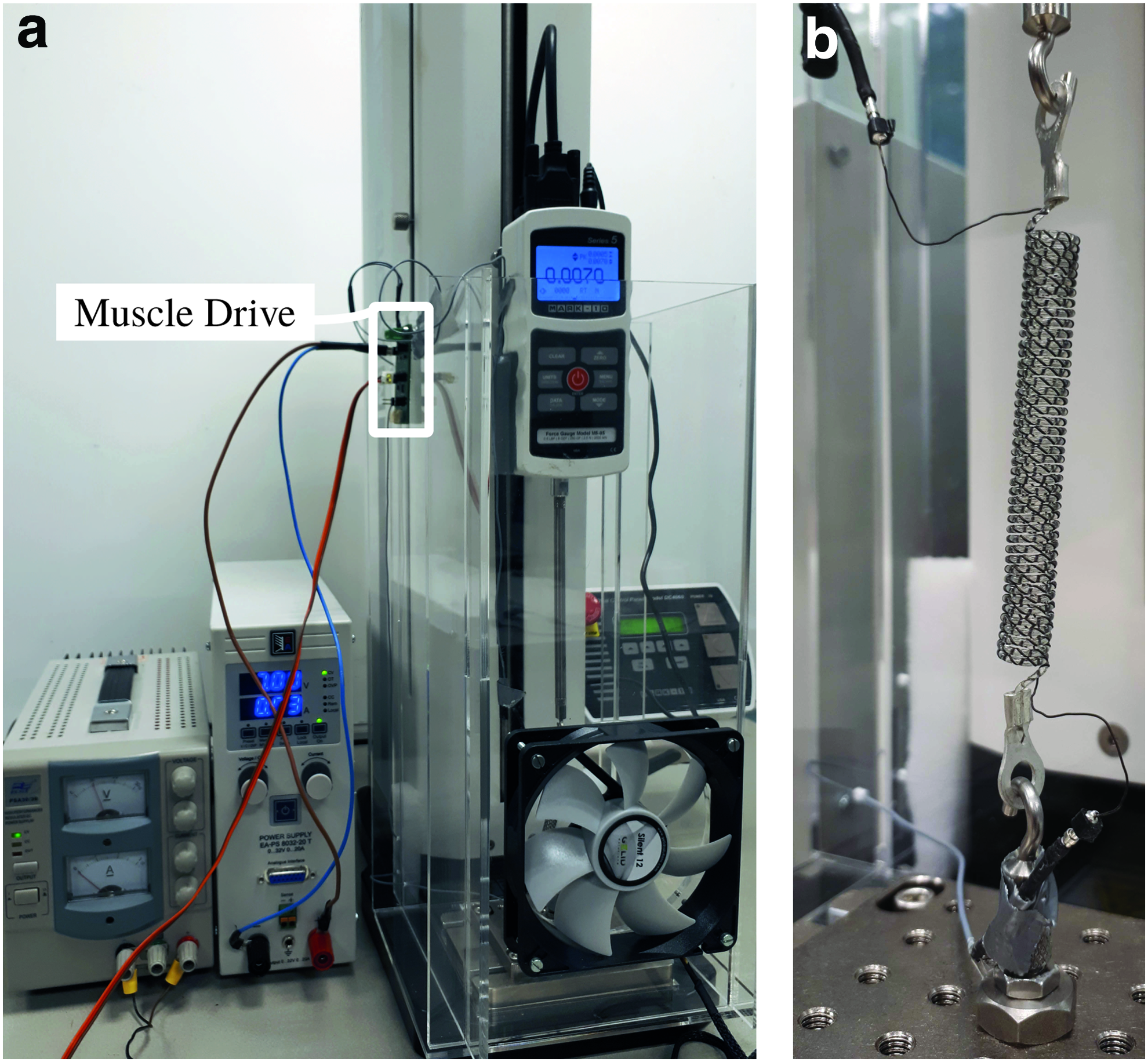
Overall setup, with the UTM and the MD in (a), and the twisted and coiled polymer muscle in (b). Color images are available online.

Muscle construction and limits

For construction of the TCPM we use the method described in our previous work²³: We align the precursor fiber and resistance wire, with a load suspended at one end, blocking rotation, and a rotary motor at the other. We twist the line until it just starts to coil upon itself. Complete coiling can be achieved either by letting the whole fiber coil upon itself or by wrapping it around a mandrel. We choose the latter, for it increases the sensitivity of inductance to muscle deflection. Annealing finishes the muscle. The endings of the resistance wire connected to the electrical leads are shaped such that when the TCPM is under tension, their influence on the force measurement is minimal. The relevant specifications for construction are shown in Table 1.

Table 1.

Muscle Construction Specifications

Property	Value
Precursor fiber diameter	0.8 mm
Precursor fiber material	Nylon
Resistance wire diameter	0.3 mm
Resistance wire material	Constantan
Load at twisting	≈6.50 N
Mandrel diameter	5 mm
Mandrel length	50 mm
Annealing temperature	165°C
Annealing time	1 h
No. of windings	46
Joule-heating resistance	10.18 Ω
Joule-heating inductance	≈1.30 μH

To obtain repeatable actuation behavior we had to train the muscle.²³ In addition, in pilot experiments we found that trained muscles that had been inactive for a while needed a warming up to regain that same behavior. Therefore, we included a warming-up phase each time we started an experiment and when we continued an experiment after a pause in the protocol.

Through pilot experiments we determined the following limits of deflection and power. To be sure to have overcome the preload knee and avoid nonlinear behavior due to touching coils,^25,31 we choose \documentclass{aastex}\usepackage{amsbsy}\usepackage{amsfonts}\usepackage{amssymb}\usepackage{bm}\usepackage{mathrsfs}\usepackage{pifont}\usepackage{stmaryrd}\usepackage{textcomp}\usepackage{portland, xspace}\usepackage{amsmath, amsxtra}\usepackage{upgreek}\pagestyle{empty}\DeclareMathSizes{10}{9}{7}{6}\begin{document} $${x_{{ \rm{min}}}} = 10\,{ \rm{mm}}$$ \end{document} as the minimum deflection for the experiments. To prevent overstretching, we choose \documentclass{aastex}\usepackage{amsbsy}\usepackage{amsfonts}\usepackage{amssymb}\usepackage{bm}\usepackage{mathrsfs}\usepackage{pifont}\usepackage{stmaryrd}\usepackage{textcomp}\usepackage{portland, xspace}\usepackage{amsmath, amsxtra}\usepackage{upgreek}\pagestyle{empty}\DeclareMathSizes{10}{9}{7}{6}\begin{document} $${x_{{ \rm{max}}}} = 30\,{ \rm{mm}}$$ \end{document} as the maximum deflection. With a voltage of \documentclass{aastex}\usepackage{amsbsy}\usepackage{amsfonts}\usepackage{amssymb}\usepackage{bm}\usepackage{mathrsfs}\usepackage{pifont}\usepackage{stmaryrd}\usepackage{textcomp}\usepackage{portland, xspace}\usepackage{amsmath, amsxtra}\usepackage{upgreek}\pagestyle{empty}\DeclareMathSizes{10}{9}{7}{6}\begin{document} $${U_{ \rm{b}}} = 7 \;{ \rm{V}}$$ \end{document} applied on the electrical leads, and a resistance at the connectors of \documentclass{aastex}\usepackage{amsbsy}\usepackage{amsfonts}\usepackage{amssymb}\usepackage{bm}\usepackage{mathrsfs}\usepackage{pifont}\usepackage{stmaryrd}\usepackage{textcomp}\usepackage{portland, xspace}\usepackage{amsmath, amsxtra}\usepackage{upgreek}\pagestyle{empty}\DeclareMathSizes{10}{9}{7}{6}\begin{document} $${R_{ \rm{b}}} = 10.75 \; \Omega$$ \end{document} , of which the resistance at the muscle is \documentclass{aastex}\usepackage{amsbsy}\usepackage{amsfonts}\usepackage{amssymb}\usepackage{bm}\usepackage{mathrsfs}\usepackage{pifont}\usepackage{stmaryrd}\usepackage{textcomp}\usepackage{portland, xspace}\usepackage{amsmath, amsxtra}\usepackage{upgreek}\pagestyle{empty}\DeclareMathSizes{10}{9}{7}{6}\begin{document} $${R_{ \rm{m}}} = 10.18 \; \Omega$$ \end{document} , the maximum power input would be 4.31 W. However, to prevent overheating, we choose an 85% duty cycle as the maximum, obtaining \documentclass{aastex}\usepackage{amsbsy}\usepackage{amsfonts}\usepackage{amssymb}\usepackage{bm}\usepackage{mathrsfs}\usepackage{pifont}\usepackage{stmaryrd}\usepackage{textcomp}\usepackage{portland, xspace}\usepackage{amsmath, amsxtra}\usepackage{upgreek}\pagestyle{empty}\DeclareMathSizes{10}{9}{7}{6}\begin{document} $${P_{{ \rm{max}}}} = 3.12 \;{ \rm{W}}$$ \end{document} . In addition, the MD requires a minimum duty cycle of 15% to provide accurate measurements. This is a practical limitation of the MD, when combined with a constantan wire for Joule heating. This sets the lower limit at \documentclass{aastex}\usepackage{amsbsy}\usepackage{amsfonts}\usepackage{amssymb}\usepackage{bm}\usepackage{mathrsfs}\usepackage{pifont}\usepackage{stmaryrd}\usepackage{textcomp}\usepackage{portland, xspace}\usepackage{amsmath, amsxtra}\usepackage{upgreek}\pagestyle{empty}\DeclareMathSizes{10}{9}{7}{6}\begin{document} $${P_{{ \rm{min}}}} = 0.10 \;{ \rm{W}}$$ \end{document} . Therefore, the boundaries within which we performed the experiments are [10, 30] mm for deflection and \documentclass{aastex}\usepackage{amsbsy}\usepackage{amsfonts}\usepackage{amssymb}\usepackage{bm}\usepackage{mathrsfs}\usepackage{pifont}\usepackage{stmaryrd}\usepackage{textcomp}\usepackage{portland, xspace}\usepackage{amsmath, amsxtra}\usepackage{upgreek}\pagestyle{empty}\DeclareMathSizes{10}{9}{7}{6}\begin{document} $$[ 0.10 , 3.12 ] \;{ \rm{W}}$$ \end{document} for power.

Signal construction

In training, warming up, identification, and validation, we excited the muscle by letting the MD apply a power, and the UTM apply a deflection. We used two signal types: a multi-sine signal m and a random-step signal g.

We constructed the multi-sine signal with N components as: \documentclass{aastex}\usepackage{amsbsy}\usepackage{amsfonts}\usepackage{amssymb}\usepackage{bm}\usepackage{mathrsfs}\usepackage{pifont}\usepackage{stmaryrd}\usepackage{textcomp}\usepackage{portland, xspace}\usepackage{amsmath, amsxtra}\usepackage{upgreek}\pagestyle{empty}\DeclareMathSizes{10}{9}{7}{6}\begin{document} \begin{align*} m{ \kern 1pt} { \kern 1pt} ( t ) = {a_0} + \mathop \sum \limits_{i = 1}^N {{a_i}} \sin \, ( 2 \pi {f_i}t + { \phi _i} ) { \rm{ , }} \tag{11} \end{align*} \end{document}

with a₀ the signal offset, a_i the amplitude of the ith component, f_i its frequency, and ϕ _i its phase. In construction, we determine the phases as: \documentclass{aastex}\usepackage{amsbsy}\usepackage{amsfonts}\usepackage{amssymb}\usepackage{bm}\usepackage{mathrsfs}\usepackage{pifont}\usepackage{stmaryrd}\usepackage{textcomp}\usepackage{portland, xspace}\usepackage{amsmath, amsxtra}\usepackage{upgreek}\pagestyle{empty}\DeclareMathSizes{10}{9}{7}{6}\begin{document} \begin{align*} { \phi _i } = { \phi _0 } - \frac { { \pi { i^2 } } } { N } { \rm { , } } \tag { 12 } \end{align*} \end{document}

where ϕ₀ is a pseudo-randomly chosen phase offset. This construction method avoids high peaks.³² We took equal amplitudes, with the signal scaled such that it fit the deflection and power limits, respectively. The frequency interval from which we took the N equally spaced frequencies was \documentclass{aastex}\usepackage{amsbsy}\usepackage{amsfonts}\usepackage{amssymb}\usepackage{bm}\usepackage{mathrsfs}\usepackage{pifont}\usepackage{stmaryrd}\usepackage{textcomp}\usepackage{portland, xspace}\usepackage{amsmath, amsxtra}\usepackage{upgreek}\pagestyle{empty}\DeclareMathSizes{10}{9}{7}{6}\begin{document} $$[ {10^{ - 2.4}} , {10^{ - 1.1}} ] \;{ \rm{Hz}}$$ \end{document} . To avoid producing the same signal for deflection and power, we took two different prime numbers for N and produced two different values for ϕ₀. For the deflection excitation we chose N = 11, and for the power excitation we took N = 7.

We constructed the random-step signal with H steps as: \documentclass{aastex}\usepackage{amsbsy}\usepackage{amsfonts}\usepackage{amssymb}\usepackage{bm}\usepackage{mathrsfs}\usepackage{pifont}\usepackage{stmaryrd}\usepackage{textcomp}\usepackage{portland, xspace}\usepackage{amsmath, amsxtra}\usepackage{upgreek}\pagestyle{empty}\DeclareMathSizes{10}{9}{7}{6}\begin{document} \begin{align*} g ( t ) = {b_0} + \mathop \sum \limits_{i = 1}^H {{b_i}} h ( t - { \tau _i} ) \tag{13} \end{align*} \end{document}

with h representing the Heaviside step function, b₀ the signal offset, b_i the amplitude for each step, and τ_i the step times. We determined the step times with a random generator, following the construction of step times for generalized binary noise.³³ Given a certain process time constant τ_p and sampling frequency f_s, for each sample time, the probability p the signal switches is: \documentclass{aastex}\usepackage{amsbsy}\usepackage{amsfonts}\usepackage{amssymb}\usepackage{bm}\usepackage{mathrsfs}\usepackage{pifont}\usepackage{stmaryrd}\usepackage{textcomp}\usepackage{portland, xspace}\usepackage{amsmath, amsxtra}\usepackage{upgreek}\pagestyle{empty}\DeclareMathSizes{10}{9}{7}{6}\begin{document} \begin{align*} p = 1 - \frac { 1 } { { 0.5 { \tau _p } { f_s } } } { \rm { , } } \tag { 14 } \end{align*} \end{document}

such that the average time between switching was half the process time constant. Via pilot experiments, we determined the approximate time constants for deflection and power to be, respectively, \documentclass{aastex}\usepackage{amsbsy}\usepackage{amsfonts}\usepackage{amssymb}\usepackage{bm}\usepackage{mathrsfs}\usepackage{pifont}\usepackage{stmaryrd}\usepackage{textcomp}\usepackage{portland, xspace}\usepackage{amsmath, amsxtra}\usepackage{upgreek}\pagestyle{empty}\DeclareMathSizes{10}{9}{7}{6}\begin{document} $${ \tau _p} \approx 2 \;{ \rm{s}}$$ \end{document} and \documentclass{aastex}\usepackage{amsbsy}\usepackage{amsfonts}\usepackage{amssymb}\usepackage{bm}\usepackage{mathrsfs}\usepackage{pifont}\usepackage{stmaryrd}\usepackage{textcomp}\usepackage{portland, xspace}\usepackage{amsmath, amsxtra}\usepackage{upgreek}\pagestyle{empty}\DeclareMathSizes{10}{9}{7}{6}\begin{document} $${ \tau _p} \approx 35 \;{ \rm{s}}$$ \end{document} . However, to not let the influence of deflection dominate in the identification data set, we chose the time constants for deflection and power to be, respectively, \documentclass{aastex}\usepackage{amsbsy}\usepackage{amsfonts}\usepackage{amssymb}\usepackage{bm}\usepackage{mathrsfs}\usepackage{pifont}\usepackage{stmaryrd}\usepackage{textcomp}\usepackage{portland, xspace}\usepackage{amsmath, amsxtra}\usepackage{upgreek}\pagestyle{empty}\DeclareMathSizes{10}{9}{7}{6}\begin{document} $${ \tau _p} = 12.5 \;{ \rm{s}}$$ \end{document} and \documentclass{aastex}\usepackage{amsbsy}\usepackage{amsfonts}\usepackage{amssymb}\usepackage{bm}\usepackage{mathrsfs}\usepackage{pifont}\usepackage{stmaryrd}\usepackage{textcomp}\usepackage{portland, xspace}\usepackage{amsmath, amsxtra}\usepackage{upgreek}\pagestyle{empty}\DeclareMathSizes{10}{9}{7}{6}\begin{document} $${ \tau _p} = 20 \;{ \rm{s}}$$ \end{document} . For the size and direction of the step, we used two pseudo-random processes. First, we sampled the step size from a uniform distribution \documentclass{aastex}\usepackage{amsbsy}\usepackage{amsfonts}\usepackage{amssymb}\usepackage{bm}\usepackage{mathrsfs}\usepackage{pifont}\usepackage{stmaryrd}\usepackage{textcomp}\usepackage{portland, xspace}\usepackage{amsmath, amsxtra}\usepackage{upgreek}\pagestyle{empty}\DeclareMathSizes{10}{9}{7}{6}\begin{document} $$\left[ {0 , 0.25 \left( {{g_{{ \rm{max}}}} - {g_{{ \rm{min}}}}} \right) } \right]$$ \end{document} , with \documentclass{aastex}\usepackage{amsbsy}\usepackage{amsfonts}\usepackage{amssymb}\usepackage{bm}\usepackage{mathrsfs}\usepackage{pifont}\usepackage{stmaryrd}\usepackage{textcomp}\usepackage{portland, xspace}\usepackage{amsmath, amsxtra}\usepackage{upgreek}\pagestyle{empty}\DeclareMathSizes{10}{9}{7}{6}\begin{document} $${g_{{ \rm{max}}}}$$ \end{document} and \documentclass{aastex}\usepackage{amsbsy}\usepackage{amsfonts}\usepackage{amssymb}\usepackage{bm}\usepackage{mathrsfs}\usepackage{pifont}\usepackage{stmaryrd}\usepackage{textcomp}\usepackage{portland, xspace}\usepackage{amsmath, amsxtra}\usepackage{upgreek}\pagestyle{empty}\DeclareMathSizes{10}{9}{7}{6}\begin{document} $${g_{{ \rm{min}}}}$$ \end{document} representing the upper and lower limit of deflection and power, respectively. Next, a virtual coin toss determined the direction of the step. However, if a step in either direction would take the signal out of bounds, the opposite direction was chosen. Finally, we scaled the signal to include the upper and lower limits of deflection and power.

Control tasks

We performed several control tasks to quantify the self-sensing performance and the closed-loop control performance of the muscle. We had the muscle perform both force and deflection control. Both consisted of step responses to determine control behavior, and tracking sinusoid references to find the bandwidth of the actuator. The step references contained seven steps, spread over the respective ranges of \documentclass{aastex}\usepackage{amsbsy}\usepackage{amsfonts}\usepackage{amssymb}\usepackage{bm}\usepackage{mathrsfs}\usepackage{pifont}\usepackage{stmaryrd}\usepackage{textcomp}\usepackage{portland, xspace}\usepackage{amsmath, amsxtra}\usepackage{upgreek}\pagestyle{empty}\DeclareMathSizes{10}{9}{7}{6}\begin{document} $$[ 0.375 , 0.525 ] \;{ \rm{N}}$$ \end{document} and \documentclass{aastex}\usepackage{amsbsy}\usepackage{amsfonts}\usepackage{amssymb}\usepackage{bm}\usepackage{mathrsfs}\usepackage{pifont}\usepackage{stmaryrd}\usepackage{textcomp}\usepackage{portland, xspace}\usepackage{amsmath, amsxtra}\usepackage{upgreek}\pagestyle{empty}\DeclareMathSizes{10}{9}{7}{6}\begin{document} $$[ 10 , 30 ] \,{ \rm{mm}}$$ \end{document} . Each step was held for 20 s. The sinusoid reference swept over 15 subsequently applied frequencies. For force control the sinusoid had a 0.05 N amplitude and a 0.40 N offset. For deflection control the sinusoid had an amplitude of 5 mm, and an offset of 20 mm. The frequencies were logarithmically spaced within the same frequency interval used for the multi-sine identification signal. The application of each frequency lasted for three periods. In pilot experiments, we tuned the gains of both controllers, via the Ziegler-Nichols method.³⁴ For deflection control, we used PID control, with \documentclass{aastex}\usepackage{amsbsy}\usepackage{amsfonts}\usepackage{amssymb}\usepackage{bm}\usepackage{mathrsfs}\usepackage{pifont}\usepackage{stmaryrd}\usepackage{textcomp}\usepackage{portland, xspace}\usepackage{amsmath, amsxtra}\usepackage{upgreek}\pagestyle{empty}\DeclareMathSizes{10}{9}{7}{6}\begin{document} $${K_{ \rm{p}}} = - 1.08 \;{ \rm{W}} / { \rm{mm}} , \;{T_{ \rm{d}}} = 0.625 \;{ \rm{s}}$$ \end{document} , and \documentclass{aastex}\usepackage{amsbsy}\usepackage{amsfonts}\usepackage{amssymb}\usepackage{bm}\usepackage{mathrsfs}\usepackage{pifont}\usepackage{stmaryrd}\usepackage{textcomp}\usepackage{portland, xspace}\usepackage{amsmath, amsxtra}\usepackage{upgreek}\pagestyle{empty}\DeclareMathSizes{10}{9}{7}{6}\begin{document} $${T_{ \rm{i}}} = 2.5 \;{ \rm{s}}$$ \end{document} . For force control, we chose to use proportional-integral (PI) control, with \documentclass{aastex}\usepackage{amsbsy}\usepackage{amsfonts}\usepackage{amssymb}\usepackage{bm}\usepackage{mathrsfs}\usepackage{pifont}\usepackage{stmaryrd}\usepackage{textcomp}\usepackage{portland, xspace}\usepackage{amsmath, amsxtra}\usepackage{upgreek}\pagestyle{empty}\DeclareMathSizes{10}{9}{7}{6}\begin{document} $${K_{ \rm{p}}} = 540 \;{ \rm{W / N}}$$ \end{document} and \documentclass{aastex}\usepackage{amsbsy}\usepackage{amsfonts}\usepackage{amssymb}\usepackage{bm}\usepackage{mathrsfs}\usepackage{pifont}\usepackage{stmaryrd}\usepackage{textcomp}\usepackage{portland, xspace}\usepackage{amsmath, amsxtra}\usepackage{upgreek}\pagestyle{empty}\DeclareMathSizes{10}{9}{7}{6}\begin{document} $${T_{ \rm{i}}} = 1 \;{ \rm{s}}$$ \end{document} . During the control tasks, the UTM imposed deflection and force, respectively. For deflection control, we had the UTM maintain a constant force of 0.40 N. For force control, we had the UTM maintain a deflection of 20 mm.

As part of the control tasks, we implemented a calibration sequence for deflection measurements and force estimates. The calibration provided two offsets, compensating for unmodeled effects, and disturbances happening in between identification and control. For calibration of the deflection measurements, the UTM held a deflection of 20 mm. The difference between the deflection estimate and the actual deflection, averaged over 10 s, gave the calibration offset for the deflection measurements. For calibration of the force estimates, the UTM held a force of 0.40 N, whereas the MD controlled the deflection. The difference between the force estimate and the actual force, averaged over 30 s, gave the calibration offset for the force estimates.

Experimental protocol

For training, we first suspended the untrained TCPM and set the load cell to zero. We then attached the bottom of the TCPM to the UTM, and we set the position of the UTM, such that the TCPM just started to be under tension. At this point, we set the deflection of the UTM to zero. Then, we turned on the fan and the MD, and we started the training. We excited deflection and power for 600 s, using a multi-sine signal for both.

The identification was initiated in the same way as training. Before gathering identification data, we gave the TCPM a warming up by means of a multi-sine on deflection and power, lasting for 250 s. For identification, we subsequently applied a multi-sine, and a random-step signal on both deflection and power, both lasting 200 s. For validation of the identification, we used a multi-sine for 100 s, followed by a random-step signal for 120 s, applied to both deflection and power. Directly after gathering identification data and preceding the control tasks, we identified the model parameters as described in the next paragraph. During this time, the TCPM was still suspended in the UTM.

The control tasks were preceded with warming up the TCPM by means of a multi-sine for 380 s, and a random-step signal for 200 s, applied on both deflection and power. After the warm-up, we calibrated the deflection measurements and force estimates. Next, we started the force-control tasks. After completion, we recalibrated the deflection measurements and force estimates, to correct for numeric drifting or low-frequency effects that were not included in the models. We then continued the experiment with the position control tasks.

Data processing

The data acquired by the UTM and the MD had their own respective time stamps. Using those, we aligned and re-sampled both UTM and MD data to 16 Hz.

To identify the 6 parameters for Equations (1), (5), and (6), we minimized the squared error between the measured and estimated force response. We obtained the estimated force response by running a simulation of the dynamical system, with the re-sampled power and deflection as input. With MATLAB's genetic-algorithm optimization, we came close to the absolute minimum. Subsequently, with MATLAB's nonlinear least-squares optimization, via the Levenberg-Marquardt algorithm, we found the absolute minimum. We found the three parameters for Equation (4) in a similar fashion, minimizing the squared error between estimated and applied deflection.

For analysis of the models, we first calculated the root mean square error (RMSE) to quantify the estimation error of deflection and force. Second, we assessed the quality of the fit via the R² value, given by: \documentclass{aastex}\usepackage{amsbsy}\usepackage{amsfonts}\usepackage{amssymb}\usepackage{bm}\usepackage{mathrsfs}\usepackage{pifont}\usepackage{stmaryrd}\usepackage{textcomp}\usepackage{portland, xspace}\usepackage{amsmath, amsxtra}\usepackage{upgreek}\pagestyle{empty}\DeclareMathSizes{10}{9}{7}{6}\begin{document} \begin{align*} { R^2 } = 1 - { \frac { \sum \nolimits_ { i = 1 } ^n { { { ( { y_i } - { f_i } ) } ^2 } } } { \sum \nolimits_ { i = 1 } ^n { { { ( { y_i } - \bar y ) } ^2 } } } } { \rm { , } } \tag { 15 } \end{align*} \end{document}

where y_i are the n data points with \documentclass{aastex}\usepackage{amsbsy}\usepackage{amsfonts}\usepackage{amssymb}\usepackage{bm}\usepackage{mathrsfs}\usepackage{pifont}\usepackage{stmaryrd}\usepackage{textcomp}\usepackage{portland, xspace}\usepackage{amsmath, amsxtra}\usepackage{upgreek}\pagestyle{empty}\DeclareMathSizes{10}{9}{7}{6}\begin{document} $$\bar y$$ \end{document} as their mean, and f_i the estimates. We calculated the R² and RMSE values for the offline estimates belonging to the identification and validation part, and online estimates of the control tasks. In addition, we calculated the 95% confidence interval for online estimation of both deflection and force. We used the data gathered during deflection control to assess deflection estimates, and data gathered during force control to assess force estimates.

To take a closer look at the performance and limitations of control, we calculated the rise times of the step responses. In addition, to determine the bandwidth of the actuator, we fit the amplitude, phase, and offset of a sinusoid with a given frequency to the respective responses to the last two periods of the sinusoid reference. We approximated the bandwidth by determining the −3 dB point via linear interpolation of the resulting magnitudes.

Results

Figure 5 shows the time series of the identification and validation experiment. Table 2 gives the fitted parameters for Equations (1), (4), (5), and (6). Table 3 shows the quality of the fit and the estimation error resulting from these parameters.

FIG. 5.

Time series of the identification and validation. The top figure shows the applied power. The middle figure shows the applied deflection in black and the fit deflection estimate in red. The bottom figure shows the measured force in black and the fit force in red. In all figures, the black vertical line shows the separation of identification and validation data. Color images are available online.

Table 2.

Fitted Parameters for Measuring Deflection and Estimating Force. The Unit at ^*Proportionally Relates to μHmm. The Unit at ^**Proportionally Relates to μH.

x		F
λ_x	2.81^*	κ_P	7.2 10⁻³ N/J	k ₁	10.8 10⁻³ N/mm
λ_l	28.8 mm	κ_c	131.6 10⁻³ 1/s	k ₂	2.7 10⁻³ N/mm
λ_o	0.433^**	F _o	106.9 10⁻³ N	c	4.3 10⁻³ Ns/mm

Table 3.

Fit Quality Measures for Deflection and Force, for Data Regarding Fitting, Validation, and Control

	Fit		Validation		Control
	R²	RMSE	R²	RMSE	R²
x	0.96	0.97 mm	1.00	0.39 mm	0.93	1.10 mm
F	0.97	12.8 mN	0.98	12.7 mN	0.86	16.3 mN

RMSE, root mean square error.

Figure 6 highlights the online estimation of deflection and force, by directly comparing the estimates with the true values. We achieved 95% confidence intervals of, respectively, 2.14 mm around a mean error of −0.27 mm for deflection estimation and 29.0 mN around a mean error of 7.5 mN for force estimation. Figure 7 shows the resulting time series of the control experiment. Herein, Figure 7a and b show the step responses during deflection and force control, respectively. Figure 7c and d show four representative periods of the respective sine sweeps. In Figure 8, we show the frequency responses of the sine sweeps during deflection control and during force control. The step responses during deflection control had rise times between 4.2 and 14.1 s, and during force control they had rise times between 2.1 and 5.1 s. Both ranges had outliers at 20 s, indicating that the response did not reach the reference value. We found the bandwidth for deflection control to be ∼1/25 Hz, and for force control to be ∼1/18 Hz.

FIG. 6.

Estimation data during, respectively, deflection control (a) and force control (b). The gray dots represent the estimates given at the true value. The red line represents the bisector of the graph, indicating what the correct values would be. The area between the black lines indicates the 95% confidence interval, which is ±2.14 mm around a mean error of −0.27 mm for deflection and ±29.0 mN around a mean error of 7.5 mN for force. Color images are available online.

FIG. 7.

Time series data regarding the control experiment. The top figures show the step responses with, respectively, deflection control (a) and force control (b) over time. The bottom figures show four sample periods during the sine sweep with, respectively, deflection control (c) and force control (d). In all four figures, the black solid line indicates the true value, the red line indicates the estimate, and the dashed black line indicates the reference. Color images are available online.

FIG. 8.

Frequency response data of the sine sweeps, with deflection control in black and force control in red. The cross markers indicate the measured response. The dashed lines indicate the linear interpolation between these points. This shows that the −3 dB point for deflection control lies at approximately 1/18 Hz, and for force control it lies approximately at 1/25 Hz. Color images are available online.

Discussion

Our method and implementation of self-sensing resulted in a 95% confidence interval of 2.14 mm around a mean error of −0.27 mm for estimation of deflection and of 29.0 mN around a mean error of 7.5 mN for estimation of force. Combined with our control implementation, we achieved a 1/25 Hz for deflection control and a 1/18 Hz for force control.

The RMSE and 95% confidence interval we achieved for estimation of deflection were sufficient for feedback control. From these results, we conclude that our measurement model in Equation (4) includes the most important effects. Still, tailoring the hardware to the range of inductance of this specific muscle would likely improve the measurements. In addition, we needed an averaging filter and a rather strong median filter to avoid spikes in the data. These artifacts should be taken care of in a new version of the hardware. Further, in the measurement model, we neglected the potential influence of the applied control signal and the influence of temperature. The former requires additional research, in combination with developments in hardware. The latter requires a measurement of temperature, for example via resistance, as in our previous work.²³

The presented implementation for force estimation also captures the most important effects, and it allows for feedback control. However, it does need improvement of both precision and accuracy. The force estimates in Figure 7b and Figure 7d show underestimation at the bottom edge of the achievable force interval, when the control signal is at the lower saturation limit. This indicates that the experimental procedure to find the Joule-heating parameters might underestimate the contribution by convective cooling. Moreover, the peaks in deflection measurements propagate in the force estimate. This explains the peaks in Figure 7b. In additional future work, we aim at quantifying the repeatability of the behavior of the muscles, both within and between muscles. We included a warming-up phase in the experimental protocol, to ensure repeatable behavior. The muscle seems to have a relaxation effect with a low time constant. Endurance tests will reveal this time constant. Subsequent modeling thereof allows for omission of the warming up.

Figure 7a and b illustrate the response of the muscle to step inputs on the reference during, respectively, deflection and force control. The rise times vary from 2.1 to 14.1 s, excluding outliers at 20 s. The control action gets saturated for the majority of the step responses.

Figure 8 shows a limited bandwidth, whereas a high bandwidth is beneficial for robotic applications. TCPMs inherently suffer from this issue, because in practice heating and cooling are slow processes. However, these actuators are suitable for tasks that do not require a high bandwidth. For example, in compliant structures they can slowly change the configuration or stiffness, or apply pre-tension. Further, there are possibilities to increase the bandwidth reported in this study by optimizing material properties, the activation principle, muscle configurations, and control methods. For example, we recommend using smaller-diameter fibers or a suitable configuration of several muscles, such as an antagonistic setup.^19,35 In addition, we see opportunities for improving the implementation of the activation principle by expanding the control action space. For example, active cooling stimulates muscle expansion.³⁶ Changing the cooling medium from air to liquid improves the performance as well.^17,35,37 Moreover, when the application of the actuator is known, a feedforward signal could improve the control performance.

A drawback of the TCPM is the poor scalability when considering a single muscle. Using a structure of TCPMs to perform as one actuator increases the scalability and versatility.^1,38 However, closely packing the muscle might lead to interaction of actuation and sensing. In future work, we will investigate these potential disturbances for self-sensing and actuation in muscle structures, and methods to cope with those disturbances.

Conclusion

In this study, we aimed at strengthening the position of TCPMs as a feasible actuator in inexpensive and lightweight control systems. To that end, we closed the feedback loop of a controlled TCPM via self-sensing. We estimated both the deflection and force, using the applied power and self-sensing measurements of deflection as input. Subsequently, this allowed us to control either deflection or force. We achieved a 95% confidence interval of 2.14 mm around a mean estimation error of −0.27 mm and of 29.0 mN around a mean estimation error of 7.5 mN for, respectively, deflection and force. This work validated the used sensing model, and it laid the foundation for further developments of research and hardware. It demonstrated the increase in potential of TCPMs to be the actuators in inexpensive and lightweight control systems.

Footnotes

Acknowledgments

The authors would like to thank Michael Fritschi for sharing the hardware that enables self-sensing, and for deliberation on how to get the most out of it. The authors would also like to thank Ron van Ostayen and Just Herder for their consultation regarding modeling and experiment design.

Author Disclosure Statement

No competing financial interests exist.

References

Haines

, Lima

, Li

, et al. Artificial muscles from fishing line and sewing thread. Science, 2014; 343:6173.

Haines

, Li

, Spinks

, et al. New twist on artificial muscles. Proc Natl Acad Sci U S A, 2016; 113:11709–11716.

Lamuta

, Messelot

, Tawfick

. Theory of the tensile actuation of fiber reinforced coiled muscles. Smart Mater Struct, 2018; 27:55018.

Yip

, Niemeyer

High-performance robotic muscles from conductive nylon sewing thread. In 2015 IEEE International Conference on Robotics and Automation (ICRA). IEEE, Seattle, WA, May 2015, pp. 2313–2318.

Cho

, Song

, Jung

, et al. A robotic finger driven by twisted and coiled polymer actuator. Proc SPIE, 2016; 9798.

Jafarzadeh

, Gans

, Tadesse

. Control of TCP muscles using Takagi-Sugeno-Kang fuzzy inference system. Mechatronics, 2018; 53:124–139.

Edmonds

BPR

, Trejos

. Stiffness control of a nylon twisted coiled actuator for use in mechatronic rehabilitation devices. In International Conference on Rehabilitation Robotics (ICORR). London: IEEE, 2017, pp. 1419–1424.

Zhang

, Iyer

, Simeonov

, et al. Modeling and inverse compensation of hysteresis in supercoiled polymer artificial muscles. IEEE Robot Autom Lett, 2017; 2:773–780.

, Chauhan

, Tadesse

. A novel soft actuator for the musculoskeletal system. Adv Mater Technol, 2018; 3:1700359.

10.

Sutton

, Moein

, Rafiee

, et al. Design of an assistive wrist orthosis using conductive nylon actuators. In International Conference on Biomedical Robotics and Biomechatronics (BioRob), Singapore, 2016, pp. 1074–1079.

11.

Saharan

, Sharma

, Andrade

MJD

, et al. Design of a 3D printed lightweight orthotic device based on twisted and coiled polymer muscle: iGrab hand orthosis. Proc SPIE, 2017; 10164.

12.

, Andrade

MJD

, Brahme

, et al. A reconfigurable robot with tensegrity structure using nylon artificial muscle. Proc SPIE, 2016; 9799:11.

13.

Rajendran

, Zhang

Developing a novel robotic fish with antagonistic artificial muscle actuators. In ASME Dynamic Systems and Control Conference, Tysons, VA, 2017, p. V001T30A011.

14.

Almubarak

, Tadesse

. Twisted and coiled polymer (TCP) muscles embedded in silicone elastomer for use in soft robot. Int J Intell Robot Appl, 2017; 1:352–368.

15.

Almubarak

, Tadesse

. Design and motion control of bioinspired humanoid robot head from servo motors toward artificial muscles. Proc SPIE, 2017; 10163:9.

16.

Steele

, Gho

, Campbell

, et al. The Bionic Bra: Using electromaterials to sense and modify breast support to enhance active living. J Rehabil Assist Technol Eng, 2018; 5:1–9.

17.

, Jung de Andrade

, Rome

, et al. Nylon-muscle-actuated robotic finger. Proc SPIE, 2015; 9431:12.

18.

Arakawa

, Takagi

, Tahara

, et al. Position control of fishing line artificial muscles (coiled polymer actuators) from Nylon thread. Proc SPIE, 2016; 9798:12.

19.

Suzuki

, Kamamichi

. Displacement control of an antagonistic-type twisted and coiled polymer actuator. Smart Mater Struct, 2018; 27:35003.

20.

Ono

, Masuya

, Takagi

, et al. Trajectory tracking of a one-DOF manipulator using multiple fishing line actuators by iterative learning control. In IEEE International Conference on Soft Robotics (RoboSoft). IEEE, Livorno, Italy, 2018, pp. 467–472.

21.

Masuya

, Ono

, Takagi

, et al. Feedforward control of twisted and coiled polymer actuator based on a macroscopic nonlinear model focusing on energy. IEEE Robot Autom Lett, 2018; 3:1824–1831.

22.

Kruusamäe

, Punning

, Aabloo

, et al. Self-sensing ionic polymer actuators: A review. Actuators, 2015; 4:17–38.

23.

van der Weijde

, Smit

, Fritschi

, et al. Self-sensing of deflection, force, and temperature for joule-heated twisted and coiled polymer muscles via electrical impedance. IEEE ASME Transact Mech, 2017; 22:1268–1275.

24.

Abbas

, Zhao

Twisted and coiled sensor for shape estimation of soft robots. In IEEE International Conference on Intelligent Robots and Systems, Vancouver, BC, Canada, September 2017, pp. 482–487.

25.

, Tadesse

. Modeling of the electrical resistance of TCP muscle. In ASME International Mechanical Engineering Congress and Exposition (IMECE). Tampa: ASME, 2017, p. V04AT05A024.

26.

Tang

, Li

, Liu

, et al. Coiled conductive polymer fiber used in soft manipulator as sensor. IEEE Sens J, 2018; 18:6123–6129.

27.

Fritschi

, van de Kamp

. Electrical displacement-, load- or force sensor. Patent No: NL2018591B1. 2018.

28.

Roylance

Engineering Viscoelasticity. Cambridge, MA: Massachusetts Institute of Technology, 2001, pp. 1–37.

29.

Suzuki

, Kamamichi

. Control of twisted and coiled polymer actuator with anti-windup compensator. Smart Mater Struct, 2018; 27:075014.

30.

Atherton

DP.

Nonlinear Control Engineering. Wokingham: Van Nostrand Reinhold Company, 1982.

31.

Cherubini

, Moretti

, Vertechy

, et al. Experimental characterization of thermally-activated artificial muscles based on coiled nylon fishing lines. AIP Adv, 2015; 5:067158.

32.

Schroeder

MR.

Synthesis of low-peak-factor signals and binary sequences with low autocorrelation. IEEE Transact Inform Theory, 1970; 16:85–89.

33.

Tulleken

HJ.

Generalized binary noise test-signal concept for improved identification-experiment design. Automatica, 1990; 26:37–49.

34.

Ziegler

, Nichols

. Optimum Settings for Automatic Controllers. Rochester, NY: Transactions of the ASME, 1942, pp. 759–765.

35.

Song

, Hori

. Force control of twisted and coiled polymer actuators via active control of electrical heating and forced convective liquid cooling. Adv Robot, 2018; 32:1–14.

36.

Takagi

, Arakawa

, Takeda

, et al. Position control of twisted and coiled polymer actuator using a controlled fan for cooling. Proc SPIE, 2017; 10163:8.

37.

Mirvakili

, Rafie Ravandi

, Hunter

, et al. Simple and strong: Twisted silver painted nylon artificial muscle actuated by Joule heating. Proc SPIE, 2014; 9056:10.

38.

Kianzad

, Pandit

, Lewis

, et al. Variable stiffness structure using nylon actuators arranged in a pennate muscle configuration. Proc SPIE, 2015; 9430:9430–9435.