Effects of Multiple Payload Launches on Launch Cost

Introduction

Although the waste of launch vehicle payload capacity is a known problem, ¹ little systematic work has been done to reduce it. This wastage constitutes a significant loss, with a total worldwide wastage of 654 tons of payload capacity from 2000 to 2013 to all Earth orbits. ² This represents a financial loss of ∼$10.7B (2014$).

In the most basic sense, there are 3 possible approaches to reducing wastage: Change the size of the launch vehicle, change the size of the payloads, or pack more payloads on each launch vehicle. Each of these approaches has disadvantages that adversely affect cost, reliability, or both. Changing the size of payloads represents a change in the capabilities of each individual payload, which may be objectionable for the customer. The changes required would be significant in some circumstances: In the dataset used for the analyses in this work, 466 of 672 low Earth orbit payloads have mass data less than 1,000 kg, and there are few launch vehicles that are both small and have good cost-effectiveness (cost per payload mass capacity). In fact, to some degree, these traits are mutually exclusive, as multiple cost models indicate.^2,3 Changing the size of the launch vehicle is not directly possible in most cases, although changing the launch vehicle configuration by adding or removing strap-on boosters may be possible. It is clear, however, that designing a new launch vehicle configuration for every conceivable payload is not practical. Launching multiple payloads is the best current method for reducing wastage, thereby decreasing cost. It is becoming a more popular practice, with the mean number of payloads per launch increasing from 1.45 payloads per launch in 2000 to 1.84 payloads per launch in 2013. ² Results will be presented here to show that conservatively a 50% reduction in wastage is possible by using this method.

Although multiple payload manifests have a proven track record of reducing costs, they are not without disadvantages. The most important of these is that adding multiple payload releases to a launch provides additional failure points, which lowers reliability. The potential cost of this is aggravated by the fact that additional payloads necessarily increase the total value of the payloads being launched on any single launch, and it, thus, makes the consequences of failure even more severe. In a financial sense, this increases the cost of launch insurance.

Method

In a previous work, as reported in Ref., ² the authors have determined the amount of wastage for all launch vehicles used in the 2000–2013 period for launches where complete payload mass and launch vehicle cost data were available. To determine this, it was necessary to tabulate all payloads launched during the interval, what individual launch they were launched on, and the launch vehicle used.

The problem of optimally assigning payloads to a minimum number of identical launch vehicles is simply a variation on the well-known bin packing problem, which has been studied extensively, and has a number of algorithms dedicated to solving it. ⁴ In the case that multiple types of launch vehicles are available and the objective is to assign them in such a way that the total launch cost is minimized, the problem becomes a variable bin-packing problem with fixed costs, as described in Crainic et al. ⁵ As examined in that work, an approximate algorithm is available to solve this problem, although with less accuracy than that for the classical bin-packing problem.

Although there are algorithms that provide exact solutions to the bin-packing problem,^4,6 a best-fit descending, or BFD, algorithm was chosen instead for the sake of simplicity. In this algorithm, the elements (in this case, payloads) are first sorted in descending order. Then, each payload is assigned to the fullest launch vehicle in which it can fit. If there are no launch vehicles with enough capacity remaining, another one is added. In the case where the payload is too large for the launch vehicle in question, it is not assigned and is added to an “NMC” (not mission capable) list. This algorithm will provide a solution that uses no more than 11/9 the optimal number of bins, and in the majority of cases will return the optimal number of bins. Korf cites a problem of 90 elements, with elements ranging in size from 0 to 1 million, and bin capacities of 1 million, where BFD returns the optimal solution 94.832% of the time. ⁴

Although the results from the BFD algorithm can be useful in certain scenarios, such as a user with multiple payloads selecting the cheapest launch vehicle for their needs, it cannot produce the most cost-effective results if multiple launch vehicle types are available. For this situation, Crainic et al. provide a solution with the adaptive-BFD (A-BFD) algorithm, dedicated to solving this variable bin-packing problem with fixed bin costs. Although subject to the same physical limitations on the problem as the BFD algorithm, A-BFD allows variation of the launch vehicle, in both number and type. This algorithm is very similar to BFD, as discussed earlier, with 2 additional steps. The various bin types must be sorted in increasing order of the ratio c/V, where c is the bin cost and V is the bin volume. For this problem, this ratio corresponds to the launch vehicle cost per maximum payload capacity. When a bin must be added, the bin with the best cost-effectiveness that is capable of holding the object being evaluated is added if the object cannot fit into one of the existing bins. Bins of identical c/V must then be sorted in ascending order of capacity.

Given the trend that larger launch vehicles are generally more cost-effective than smaller launch vehicles, it may seem that this approach will cause excessive wastage, especially in the last few manifests assigned. Crainic addresses this issue by introducing a postprocessing step after assignment of all payloads where the algorithm may swap each loaded bin with a new bin from the set of available bins if the second bin is less expensive and has enough capacity to hold the contents of the first bin. For instance, if a very small payload is assigned to a very large capacity launcher by itself owing to this launcher's superior cost-effectiveness in the algorithm's first pass, the postprocessing step will evaluate this situation and select the cheapest launch vehicle that is capable of launching this payload, even if its cost-effectiveness is poor.

The physical nature of the problem, however, introduces a few additional complications to the use of bin-packing algorithms. The most important of these is that launch vehicle capacity depends on the payload's desired orbit. For example, Orbital Sciences' Pegasus XL can place 450 kg into a 200 km altitude, 28.5° inclination orbit, but only 120 kg into a 1,400 km 28.5° orbit. ⁷ This means that the launch vehicles cannot be treated as simple bins; there must be a mechanism to account for the payload's orbit. Another complication follows from this. Two payloads in wildly different orbits cannot be launched together unless one of them is provided with a propulsion system or the entire vehicle delivers each payload to its destination. This is occasionally done, as demonstrated by launch 2002-042, a H-IIA 2024, which placed 2 USERS satellites into low Earth orbit (LEO) and the Kodama satellite into geosynchronous transfer orbit, but this practice is not common and in some cases it can impose significant additional ΔV requirements.

Both the problems mentioned earlier primarily affect payloads in low and medium Earth orbits. Since geosynchronous orbits are characterized by a specific orbital radius, they have very similar ΔV requirements, making them much more amenable to the bin-packing approach. Although the ΔV requirements may not be completely homogenous owing to differences in the trajectory used and/or amount of ΔV provided by the payload, they will be assumed to be so herein. For these reasons, this work will only consider geosynchronous payloads. Payload data throughout are taken from Boone and Miller. ² In the data collected by that paper, there are 358 geosynchronous payloads with payload mass data. The analyses in this article are applied to this data set and to all launch vehicles used during the 2000–2013 interval that have geosynchronous transfer orbit capacity (i.e., excluding small LEO-only launchers such as Pegasus and Falcon 1).

A final complication arises when estimating the cost of the launch. Dramatically increasing the number of payloads launched by a single launch vehicle makes the integration of payloads significantly more difficult, and it increases the associated engineering costs. Estimation of these costs is difficult, as they are heavily payload- and launcher specific even before considering the additional complexity of increasing the number of payloads. In addition, the prices given for launch vehicles often do not indicate whether or not this expense is included in the price of the launch vehicle. Finally, the logistics of assembling multiple payloads from different customers may impose additional costs. Since these costs are not amenable to estimation in a general way applying to the market as a whole, they will not be included in this analysis.

Additional constraints may apply for real-world missions and require investigation. The first is launch timing. Some payloads must launch at certain times for business or other reasons, such as ISS resupply spacecraft. Others may be less time critical, such as many scientific payloads. It is difficult to determine the time scheduler requirements for individual payloads. Therefore, separate analyses first examine a scenario with no time schedule restrictions and then examine a scenario where each payload must launch in the same calendar year that it actually launched.

The second possible restriction is launch vehicle availability. Launch vehicle types were available in different quantities over the studied interval. Although from a simple cost perspective it would be ideal to only buy the most cost-effective launch vehicles, this may not be possible in a real scenario. Similar to time schedules, it is difficult to determine how much actual production capacity exists. Therefore, separate analyses consider a scenario where there are no restrictions on launch vehicle availability and another with launch vehicle availability restricted to the launch vehicles actually used during the studied period.

Results

An example of the results for application of the BFD algorithm to all 358 payloads may be seen in Table 1. This is an excerpt from the optimal payload arrangement for the Falcon 9 v1.1 launch vehicle. Payloads are identified in Table 1 by their COSPAR identification numbers. Mass is also listed here for reference. As stated earlier, the NMC list is composed of payloads that are too heavy for the given launch vehicle to launch.

Table 2 compares wastage in actual service for launch vehicles with what is theoretically possible if the launch vehicle were to launch all geosynchronous payloads that it was capable of launching. As can be seen, most launch vehicles have much higher wastage than is theoretically possible with all payloads from the data set. Note, however, that it is possible to have a lower wastage in actual service than this minimum wastage for launching all payloads in the dataset by the simple virtue of not launching payloads that are not a good fit for the given launch vehicle. This is true for a number of launch vehicles that are indicated in Table 2 with italics. The reverse is also true; if a launch vehicle is used for payloads that are not a good fit, its wastage will be higher.

Given that sizing is an important launch vehicle design decision, it would be instructive to consider whether this theoretical minimum wastage is a function of the launcher's size. Figure 1 plots launchers' maximum geosynchronous payload capacity against wastage if the payloads were ideally packed. It is clear from Figure 1 that there is a trend in this ideal case between maximum payload capacity and wastage. Wastage dramatically decreases as payload capacity increases if payloads are optimally packed.

OPEN IN VIEWER

Fig. 1.

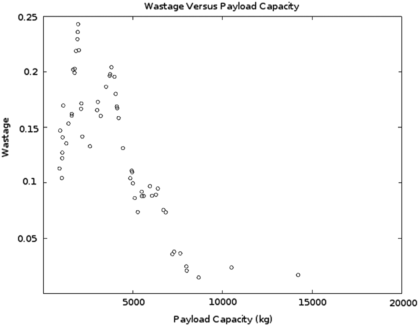
Wastage versus payload capacity.

Wastage in and of itself, however, is not a measure of merit. Since the point of reducing wastage is to reduce launch costs, it would be prudent to directly examine the relationship between cost-effectiveness (cost per payload mass delivered to orbit) and maximum payload capacity in this ideal case. Figure 2 plots this relationship by using launch vehicle prices drawn from previous work. ²

OPEN IN VIEWER

Fig. 2.

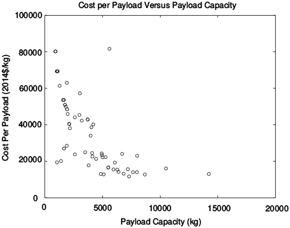
Cost per payload mass delivered versus payload capacity.

Although the results in Figure 2 provide some insight into existing launch vehicles, their usefulness for estimating the cost of payloads on prospective launch vehicle designs is limited by the inherent variations in cost-effectiveness between existing launch vehicle designs. For use in estimating the cost-effectiveness of future designs, the use of a cost model can provide some idea of future cost trends. The cost estimation model in Herrmann and Akin ⁸ , drawn from NASA's SLVLC, enabled computation of the life cycle cost (recurring, nonrecurring, and operational) for a series of launch vehicles sized in multiples of 1,000 kg, operating under the assumption that the theoretical launch vehicles would launch all payloads in the data set within their respective payload capacities.

The values for theoretical life cycle costs were computed by using the same assumptions made by Herrmann and Akin in their baseline case. Specifically, they assume a 2-stage expendable vehicle with a 425 s specific impulse, a structural fraction of 7.8%, and a first-stage ΔV fraction of 67%. The results of the bin-packing algorithm at each payload mass provides the number of launches for the computation of recurring and operational costs. Figure 3 presents results for this case.

OPEN IN VIEWER

Fig. 3.

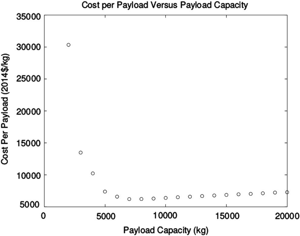
Cost per payload mass delivered versus payload capacity with life cycle cost.

As can be seen, the effect of optimally packing the launch vehicles has a minimal effect on overall trends in launch vehicle cost per payload mass delivered for medium to heavy launch vehicles. Wastage does not decrease quickly enough past 8,000 kg maximum payload capacity to offset the increasing nonrecurring costs that are associated with developing heavier and heavier launch vehicles. Below 5,000 kg payload capacity, the beneficial effects of multiple payloads become less important, as fewer and fewer of the launches in the optimal case have multiple payloads. For example, Falcon 9 v1.1 at 4,850 kg geosynchronous transfer orbit payload capacity has only 1 manifest with more than 2 payloads, and the majority only have 1. Far more important is the effect of limited capability, as touched on in a previous work. ² The 1,000 kg capacity theoretical launch vehicle can only carry 8 payloads out of the 337 in the data set, at a staggeringly high cost of $127,710 per kg delivered to the geosynchronous transfer orbit if it is only developed and used for that mission.

It is clear that the use of larger launch vehicles reduces wastage and cost in the ideally packed scenario with 1 type of launch vehicle. It is less certain, however, that this trend holds true if multiple types of launch vehicles are available, and if so, what the cost savings are. Application of the A-BFD algorithm to the full set of launchers and payloads, with minimization of cost as the goal, provides a minimum-cost scenario. Table 3 contains launch vehicle usage for this case.

As would be expected, the results emphasize more inexpensive launch vehicles. It is instructive to note, however, that capacity does play a role. The heaviest geosynchronous payload in the data set masses more than 8 tons, which is far in excess of Falcon 9 or Long March 3B's rated capacities. This drives the use of larger, more powerful, but less cost-effective launchers such as Atlas V 551. The end result is a total launch cost savings of 45% over the missions as actually launched, with a reduction in wastage from 21.8% to 9.66%.

The results obtained by using the A-BFD algorithm suggest that the “optimal” solution for any given set of launch vehicles and payloads will maximize use of the least expensive launch vehicle, subject to limitations in payload capacity. However, this presents an obvious real-world problem: availability. Even if 1 launch vehicle is far superior in terms of cost-effectiveness than any other, there is some limit as to how many could be produced. It is highly unlikely that all launch vehicle providers were producing at maximum capacity over this entire period, so some variance might not be of consequence, but the solutions mentioned earlier that only use a few types of launch vehicles present a problem.

To investigate this, it is necessary to apply the A-BFD algorithm again while forbidding the use of launch vehicles whose quantities have been exhausted. Table 4 presents launch vehicle usage if only the quantities of launch vehicles actually used for geosynchronous payloads during the studied interval were available. This scenario limits use of the most popular launchers in Table 3, especially Falcon 9, which was not actually used for any geosynchronous missions during the studied interval, and so offers lesser savings of 27.3% while reducing wastage to 4.73%.

Some missions are time critical, such as space station resupply. Although these constraints do not apply to all missions, it is necessary to investigate the effects of schedule constraints on the potential for scheduling to reduce costs. This may be done by running the algorithm on a single year's payloads and launch vehicles at a time and then summing all years in the data set. Accordingly, the analyses in Tables 3 and 4 were repeated with a requirement that each payload be launched in the same year that it was actually launched in. Tables 5 and 6 contain results for this case. For the case with an unconstrained launch vehicle selection, this reduces the total cost savings to 43.7%. If the launch vehicle selection is constrained, cost savings are reduced to 19.1%. The reduction of launch vehicle usage, and the corresponding savings, in this scenario may be seen in Table 7.

Discussion

Several conclusions may be drawn from the information presented earlier. The first is that aside from their larger potential market share, the results indicate another potential advantage that large launch vehicles have over smaller ones. The current raisons d'etre for small launch vehicles are flexibility and launching small payloads, which are actually the majority of low Earth orbit payloads. ² If payloads can be loaded without prejudice on large launch vehicles, however, their wastage is actually lower than that of small launch vehicles, increasing their already formidable cost advantage.

These results set a boundary for what a large launch vehicle is with regard to the capability to reduce wastage. Most of the potential reduction in wastage, and thus cost, is obtained at a geosynchronous transfer orbit payload capacity of ∼8,000 kg. Beyond that, only a small improvement in wastage from increasing size occurs. Since the development of ever-larger launch vehicles begins to increase the life-cycle cost per payload mass capacity of the launch vehicle, ⁹ it is clear that there is a point of diminishing returns.

The cost model shows this point of diminishing returns to be near 8,000 kg as well. Thus, given current market conditions, this represents an optimal payload capacity from a cost perspective. Only a single payload of the 337 in the data set masses more than this, and the remainder can be launched at a wastage of 2.07%. Give that some sort of payload adapters would be required to physically attach the payloads to the launch vehicle, this probably represents a practical lower limit on wastage in actual use.

In scenarios where multiple types of launch vehicles are available, several interesting trends are apparent. The first is that competition in these scenarios is very cutthroat. If launch vehicle selection and manifesting is completely free, the number of launch vehicle types used decreases from 37 to 5. Limiting the launch vehicle availability to what was actually used still reduces the launch vehicle types used to 26. Investigation of Table 4 shows that usage is very much a binary decision: Either a launch vehicle is cost-effective enough to be used, in which case all of those available are used, or it is not, in which case none are used. The sole exception in that scenario is a single Ariane 44P launch. Addition of the time constraint increases the number of types used. Only 1 launcher, Ariane 42P, is completely eliminated, although all launchers with poor cost-effectiveness suffer a reduction in numbers.

Conclusions

A significant savings in terms of launch cost is possible for most launch vehicles if multiple manifesting of payloads is increased in a systematic way. Assuming that each launch vehicle's individual market is similar to the geosynchronous market as a whole, many popular launch vehicles could reduce wastage and, thus launch cost, by a maximum of 15% of total capacity by arranging multiple manifests in a way that is designed to reduce wastage. This practice would also, in theory, promote additional savings, because it enables the use of heavier launch vehicles that usually have better cost-effectiveness. Although there is a point of diminishing returns at ∼8,000 kg of geosynchronous payload capacity, below this, the higher the launch vehicle's capacity, the better. Reducing the use of cost-ineffective small launch vehicles will result in additional savings.

If payloads could be arranged in the most cost-optimal way on the varied types of existing launch vehicles with no regard to time schedules or the number that can be produced, launch cost savings of a maximum of 45% over existing costs are possible. Placing constraints such as time schedules or availability restrictions reduces this, but even in the most restrictive case, where launcher selection is restricted to the quantities actually produced and the payload must launch on a manifest in the same year that it actually launched in, a savings of a maximum of 19% is possible over existing usage.

Both wastage and poor launch vehicle cost-effectiveness increase launch costs. These analyses show that launch vehicle cost-effectiveness is the primary driver behind high launch costs. If launch vehicle choice is unrestricted, wastage only slightly decreases as costs decrease dramatically. This is similar to the results in previous work, ² where an examination of changing launch vehicle selection for the as-launched manifests showed a significant reduction in cost without a corresponding reduction in wastage. However, if launch vehicle choice is restricted and scheduling constraints are imposed, the reduction of wastage becomes more and more important.