Multispecies Single Light-Emitting Diode Mid-Infrared Gas Sensor for Space Habitats and Vehicles

Abstract

To further extended deep space exploration missions, both through commercial space endeavors and through government-funded opportunities, the hazard of toxic gas accumulation onboard space vehicles must be quickly resolved to ensure mission success. Such events can occur due to fire events or fuel/oxidizer leaks. Several hazardous gases that are present in a space environment have absorption features in the mid-infrared range and thus can be detected and quantified via absorption spectroscopy. This work presents a benchtop sensor that utilizes a 4.2 μm light-emitting diode and a rotating diffraction grating to detect both carbon dioxide and nitrous oxide. Subsequent works will focus on adding further species of interest and post benchtop testing.

Introduction

As human curiosity expands the occupied volume within the universe, increased duration and interplanetary manned space travel will become increasingly routine. In these travel vehicles, humans, cargo, and equipment will be housed within a fixed mass atmosphere. This closed environment must be cleaned of any waste gases that occur; this includes carbon dioxide (CO₂), which can be formed from respiration, fire, or smoldering, or molecules that produce odors from everyday tasks such as cooking or brewing coffee.¹ On Earth, these gases would normally be allowed to disperse and would be quickly diluted within the ambient atmosphere or decomposed. However, in space travel, it is critical to implement and maintain a rapid early warning detection system, which can alert the occupants and trigger automated response countermeasures whenever fire or toxic gases begin to accumulate. Thus, it will be necessary to have a low volume/mass/power footprint sensor with high sensitivity and low response time to a range of species.

Residential and commercial fire detection devices are well-established featuring alpha particle-based detection schemes, which are inappropriate for space applications. These differences in detector performance are the result of combustion phenomena in the absence of gravity; false positives (alarms triggered without need) are particularly common due to debris or other nonthreatening objects.² In addition, such detectors are also unable to probe for toxic gases, requiring additional units for sensing each specific toxin.

While fixed-location smoke and hazardous gas detectors are not suitable for spacecraft, there have been some detectors, which have already been implemented in space vehicles. As recently as NASA's Apollo program, crew members senses and observations were the sole sensors responsible for troubleshooting.³ Since Apollo, NASA has advanced the use of smoke detectors using ionization smoke sensors on Skylab and using photoelectric principles within return air ducts on the International Space Station (ISS).³ Some spacecraft cabin gas sensors rely primarily on laser-based absorption spectroscopy.⁴ However, lasers are expensive and have large power consumption and sensitivity issues. Additionally, due to laser characteristics, it is necessary to have a single laser per species to be detected.⁵ Thus, to enable detection of gases which result from combustion or leaks among cooling/propellant/other systems, light-emitting diodes (LEDs) are proposed as viable alternatives as they feature significantly lower power requirements and can be implemented in broad range sensors.

The sensor design that is discussed in this work is the culmination of several previous design iterations. A preliminary design used 3 separate LEDs centered at 3.6, 4.2, and 4.7 μm along with a pair of beam splitters to allow light to pass through a single test cell.⁶ In this design (Fig. 1A), the 3.6 μm LED served as a reference while the 4.2 and 4.7 μm LEDs were used to detect CO₂ and carbon monoxide (CO), respectively. To separate the signals after they had reached the detector, the LEDs were modulated at different frequencies and a frequency-dependent demodulation was implemented. This benchtop model was downsized and utilized a single optical path (Fig. 1B) and tested on high-altitude balloon flight.⁷ A revamp of the detection system enabled the simultaneous frequency- and amplitude-modulated measurements to reveal ambient temperature (frequency shifts) and CO₂ concentration (amplitude shifts). Additionally, rather than utilize an absorption cell, the sensor was packaged in an enclosure with environment to enable measurements along the length of the optical path. The sensor and enclosure were then covered using an external aluminum enclosure to mitigate radio from terrestrial or cosmic sources.

Fig. 1.

(A) Preliminary sensor schematic.⁶ (B) Optical design for high-altitude balloon flight.⁷

The primary goal of the latest sensor design is to prove, in a laboratory benchtop environment, that the broad spectral profile of a single LED can be utilized for multispecies targeting with the use of both a reflective grating and an exit slit to enable wavelength selection. This sensor will be tested with mixtures of varying concentrations of CO₂ and nitrous oxide (N₂O) balanced in nitrogen (N₂) at room temperature and near ambient pressure.

Sensor Theory

Absorption Spectroscopy

Absorption spectroscopy is a method of using a gaseous species' dipole characteristics to quantify concentrations by examining attenuation by the gases when temperature, optical path length, and reference intensity are known.⁸ With nondispersive infrared sensors, infrared light travels from a source to a detector through a probed medium (Fig. 2A). If there are species within the medium that possess absorption features of the gas at the wavelength of the sources' emitted light, then absorption occurs. A form of the Beer–Lambert law [Eq. (1)] can then be used to relate the reference intensity $I_{λ, 0}$ (W·cm⁻²) and the transmitted intensity $I_{λ}$ (W·cm⁻²) to calculate the spectral absorbance $A (λ) e q n o o p e n (u n i t l e s s)$ .

Fig. 2.

(A) Schematic of a typical optical setup consisting of an IR source, test cell containing the species of interest, and an IR detector. (B) Comparison of light intensity at different locations along the path length: reference intensity at the source ( $I_{λ, 0, s_{0}}$ ), reference intensity at the detector ( $I_{λ, 0, s_{3}}$ ), and transmitted intensity when a gas is present in the test cell ( $I_{λ, s_{3}}$ ). IR, infrared.

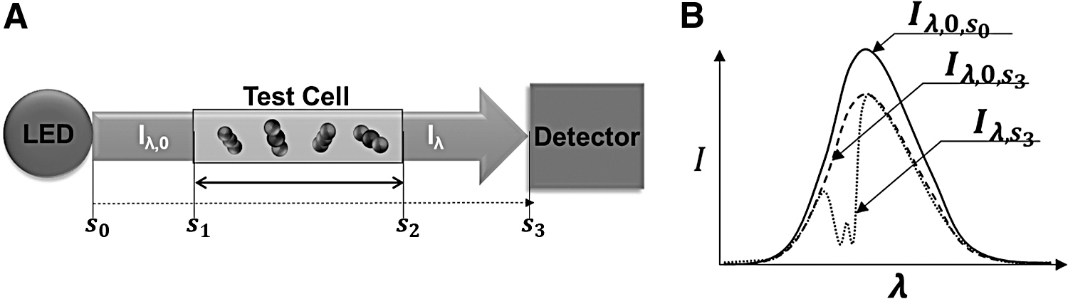
In the current setup, reference intensity is measured by the detector when the test cell is under vacuum and the transmitted intensity is measured by the detector when the test cell contains the mixtures of interest. The mole fraction of the ith species $χ_{i} e q n o o p e n (u n i t l e s s)$ can then be found provided the species concentration n_i (mol/cm³), the path length L (cm), and the wavelength-specific absorption coefficient $α_{λ, i}$ (cm⁻¹) are known. The absorption coefficient for the species being measured is further defined [Eq. (2)] and can typically be found in HITRAN or other databases. Here, $S_{λ}$ (atm⁻¹·cm⁻²) is the spectral line strength, $ϕ_{λ} e q n o o p e n (c m)$ is the line shape function, and $χ_{i} e q n o o p e n (u n i t l e s s)$ is the mole fraction of the ith species. As the absorption coefficient value varies with temperature, the temperature in the environment must be monitored for fluctuations.⁹ A simple schematic depicting spectral features is shown in Figure 2B. $A (λ) = - l n (\frac{I_{λ}}{I_{λ, 0}}) = a_{λ, i} n_{i} L$ (1)

α_{λ, i} = S_{λ} \cdot ϕ_{λ} \cdot χ_{i}

(2)

Wavelength Selection via Diffraction Gratings

One key component of this design is a reflective diffraction grating, which enables chromatic angular dispersion of light characterized by Equation (3) and schematically in Figure 3.¹⁰ In Equation (3), the order of diffraction n (unitless); in the case of the zeroth order (n = 0) the light is reflected, and while an infinite number of orders exist (0 ≤ n < ∞), intensity as order increases rapidly decays and thus the first order (n = 1) is that which is of engineering utility. Then, given the geometric grating constant d (mm), which corresponds to the size of the reflective features on the gratings surface, and the necessary angles α (incident) and β (wavelength-dependent diffracted angle), the wavelength λ (μm) that will ultimately reach the detector can be determined. In many applications involving a grating, the position of the incident light with respect to the grating will generally change to change the resulting wavelength. In the instance of an LED source, the incident light is composed of a range of wavelengths. However, in this setup, the grating itself is the moving component and all other components remain stationary; it is therefore important to move the grating in a quantifiable manner. As the grating rotates, the angles α and β now change; as a result, λ is now a different value. In this manner, a range of wavelengths from ∼3.3 to 4.7 μm can be studied with the use of a single LED. Typically, diffraction gratings are coupled using an exit slit to stop scattered light, which has spectral features far from that of the desired.

Fig. 3.

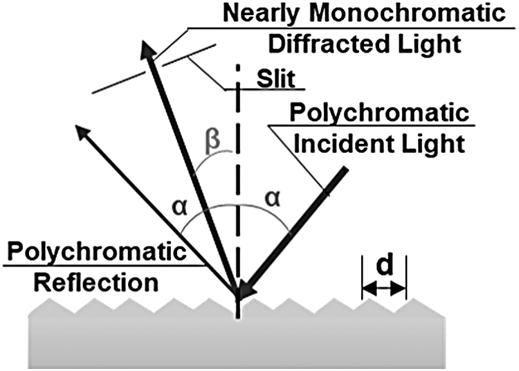
Diffraction grating diagram showing the incident light, reflected light, and one mode of diffracted light.

β = a s i n (\frac{n \cdot λ}{d} - sin (α))

(3)

Apparatus Design

This section discusses all design considerations involved in creating a sensor capable of detecting multiple species with a single LED. The Species Selection section explains the rationale for the 2 targeted species for the apparatus, and the Sensor Optical Design section depicts the optimized optical design. The optical calibration procedures are an important component in determining a feasibly repeatable model and are discussed in depth in the Sensor Grating Position Calibration section. This setup is also validated with the use of laser absorption spectroscopy; the optical design for the laser-based setup is explained in the Quantum Cascade Laser Concentration Reference Measurements section.

Species Selection

To expand the functionality of this sensor over previous designs, the principal objective is to enable multispecies detection via a single LED. For this sensor, it is to be accomplished via a benchtop setup and the implementation of a rotating diffraction grating, as this allows for separation of wavelengths from the light source in a quantifiable manner. A single LED source is used, which will enable the detection of both CO₂ (4.2 μm) and N₂O (4.5 μm). CO₂ has been the primary detected gas for previous iterations as well. N₂O is also commonly known as “laughing gas” because of its uses as a sedative in dentistry. In space applications, N₂O is an oxidizer commonly used in hybrid rockets, such as Virgin Galactic's RocketMotorTwo.¹¹ It is therefore important to monitor in case of any possible gas leaks, especially if humans are onboard.

Sensor Optical Design

Among the various manufacturers of LEDs, it is necessary to select one, which would offer sufficient intensity across the necessary wavelength ranges. A Thorlabs LED4300P is utilized and features sufficient output over the wavelength range of 3.3–4.7 μm. Relative spectral intensity can be seen in Figure 4, which demonstrates the relative intensity at 3 different temperatures. While each of the temperatures produces maximum relative intensity at ∼4.1 nm, there are slight variations that occur in the peak centerline positions. Additionally, it can be seen that output intensity across all wavelengths dramatically increases when temperature is reduced, until ∼4,300 nm; after this point, the opposite trend is seen in that intensity increases as temperature increases.

Fig. 4.

Spectral output with respect to wavelength of the LED used.¹² LED, light-emitting diode.

Within Figure 5 , the sensor schematic can be seen, which shows the collimating lenses, gas cell diffraction grating, slit, condenser lenses, and photodiode. Photons emitted from the LED are first collimated and directed through a gas cell with an internal path length of 14 cm. Polychromatic light, which is transmitted through the gas cell, is then chromatically dispersed using the grating. A condenser lens and slit pair are utilized to both ensure there is proper focus on the detector and to ensure proper biasing of wavelength selections. Within this work, the slit width was held at a span of ±0.98 mm, which allows for a wavelength transmission range of ±5.061 nm from the centerline intensity. To modulate the LED at a constant frequency of 250 kHz, a function generator (4005DDS; BK Precision) was utilized.^6,13 No additional load matching was used.

Fig. 5.

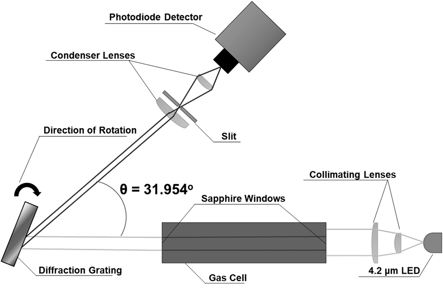
Sensor schematic showing the optical path, the LED, gas cell, rotating grating, optical slit, and photodiode detector.

Sensor Grating Position Calibration

Several important calibration procedures must be completed before species detection. As the grating has a variable position, it is important to ensure minimal jitter and drift. Here, “total range” refers to the total rotation of the grating and the corresponding wavelength range used for analysis. The grating was mounted atop a manual rotating stage (TR80; Newport) with a maximum of 6° fine rotation. For the following tests, we enabled the grating to sweep a range of 5.8° to ensure no stop issues would arise; this translated to a wavelength sweep range of 4,117–4,592 nm when using the specified LED. To automate grating rotation, a stepper motor was attached to the rotating stage's fine tuner, and the motor was driven by an Arduino Uno, which cross-references signals with a USB-6366DAQ (National Instruments). To define a reference position, a laser pointer centered at 650 nm was used to define the reference angle labeled as θ in Figure 5. The laser was placed as close to the LED and gas cell portion of the schematic as possible, as shown in Figure 6. The grating was then rotated so that it was vertically and horizontally aligned with the laser such that the incident light reflected to its source; this was further validated by comparing the distance between the diffraction modes on a flat surface with the use of a Vernier Caliper (20140428; Capri Tools). Then, after noting the angle on the rotating stage for the initial position, the grating was rotated until a mode reached the gas cell and the LED; by noting the order of the mode and the angle of rotation, φ₁, Equation (3) was used to determine the angle between the laser and the LED. Here, φ is equal to α + β. Then, the grating continued to rotate until the same mode passed through the optical slit and reached the detector; this new angle φ₂ was used to calculate the angle between the laser and the detector. Thus, θ, a reference angle between the LED and the detector, could be calculated; this process was completed several times and an average angle value of 31.954° ± 0.025° was determined.

Fig. 6.

Optical setup calibration procedure. First, φ₁ is calculated by rotating the grating until a certain mode (n = 2 in this case) reaches the LED. Then, φ₂ is calculated by continuing to rotate the grating until the same mode reaches the detector. Additional modes that are not of interest for calculation are shown to be gradually fading.

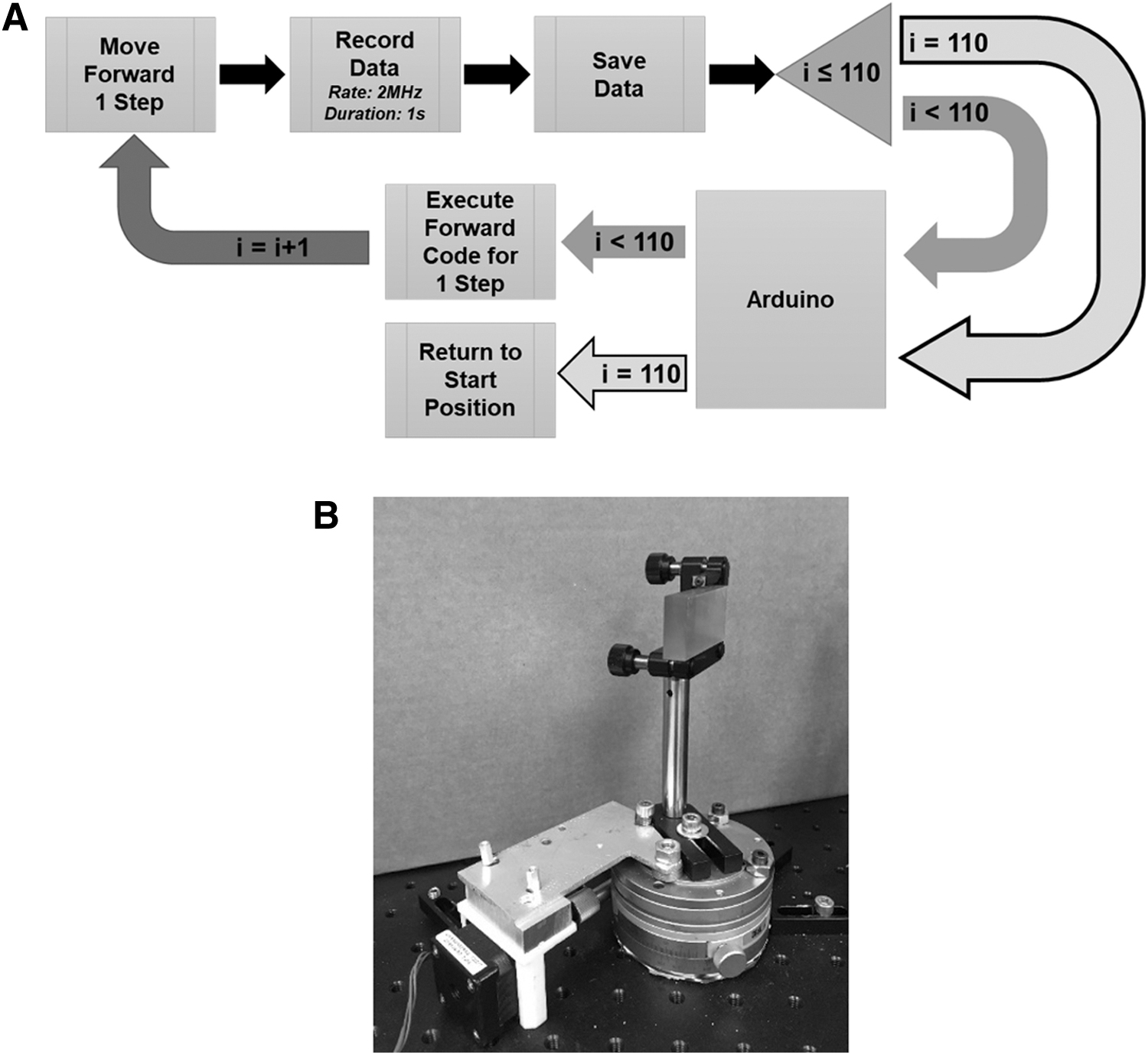
To ensure that the total range of rotation remained constant, several full-scale sweeps were performed in succession. The main potential sources for drift in this setup were within the programming and with the physical grating rotation assembly. A simplified diagram of the LabVIEW code is presented in Figure 7A. LabVIEW controlled data acquisition (DAQ) instructions sent to the Arduino, enabled the grating to rotate and then pause while data were recorded and saved. This process was repeated until the full sweep range of 5.8° was probed with a total of 110 data points. Jitter and drift testing was then conducted, in which the grating was rotated to its full test range and back to its original position 20 times in succession without any detectable deviation in start position. At the final measurement position, the Arduino commanded the grating to return to its initial position.

Fig. 7.

(A) DAQ programming logic diagram. (B) Stepper motor mounted to rotating stage. DAQ, data acquisition.

Quantum Cascade Laser Concentration Reference Measurements

Two Distributed Feedback Quantum Cascade Lasers (QD4250CM1AS and QD4580CM1; Thorlabs) were utilized to perform validation tests for this setup. The first laser, with a wavelength range of 4.256–4.266 μm, was used to measure CO₂, whereas the second contained a wavelength range of 4.583–4.596 μm and was used to measure N₂O.¹⁴ A schematic is shown in Figure 8. The signal from the 2 lasers is combined with the use of a beam splitter. This signal is then split again; 2 fiber-optic couplers are used to send the output to a spectrum analyzer (771B; Bristol) and to the setup seen in Figure 5 simultaneously. The purpose of the spectrum analyzer is so that any drift in the lasers that occurred during testing could be monitored. With this setup, the grating was first rotated such that the CO₂ laser reached the detector and then rotated such that the N₂O laser reached the detector.

Fig. 8.

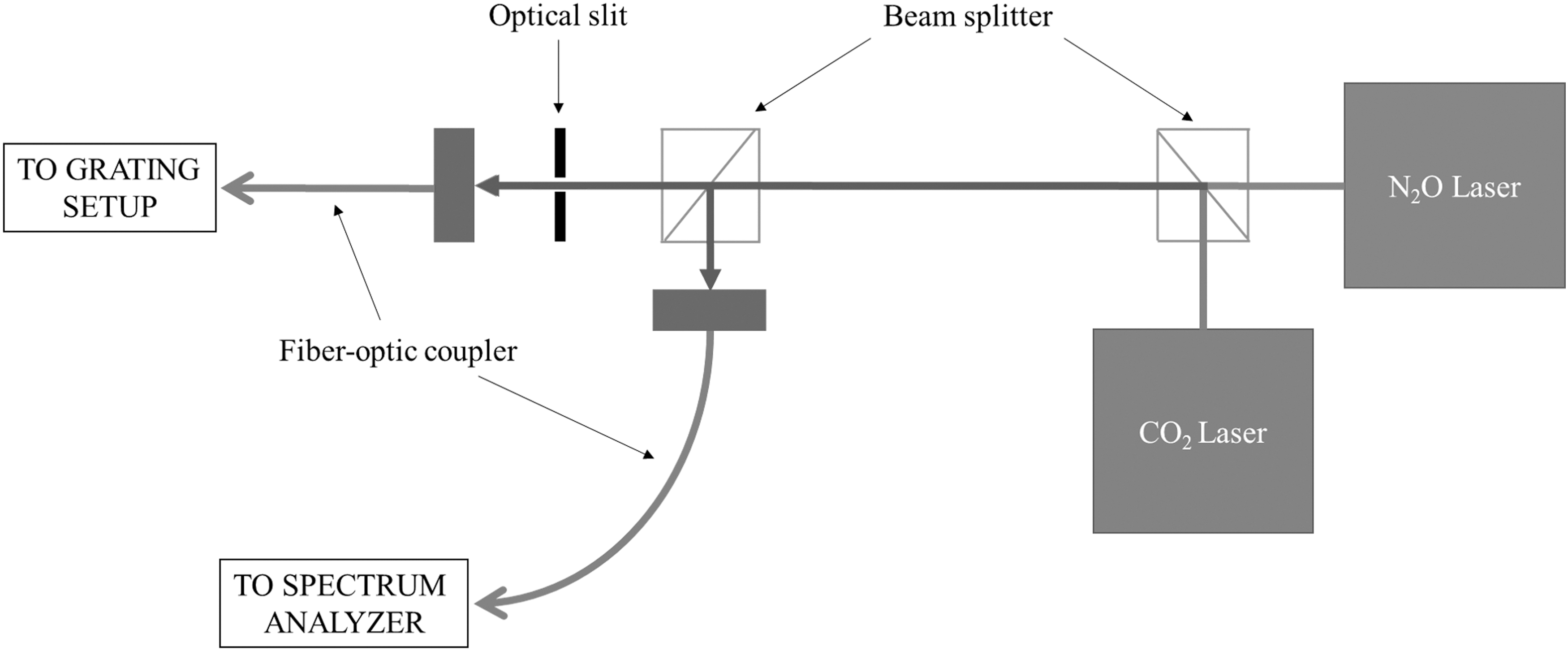
Laser setup diagram.

Data Collection and Evaluation

LED Experiment

All tests were performed within a laboratory fume hood to maintain a controlled environment and minimize potential exposure to leaks. The temperature in the fume hood environment was measured with the use of a thermistor and the Arduino. A temperature value was recorded at each step to account for any fluctuations while the tests were underway. This temperature value was used in theoretical absorbance calculations across the wavelength range [Eq. (1)]. In addition, a vacuum calibration test was taken where the test cell was in vacuum. This test served as the reference intensity to be used in the experimental absorbance calculations [Eq. (1)]. All intensity values were recorded in terms of decibels by the DAQ and were converted to a linear intensity scale for further analysis. This was carried out with the power law Equation (4). Both the reference and transmitted intensities used for calculations were normalized with respect to power fluctuations by dividing by the measured power from the function generator. $\frac{P_{2}}{P_{1}} = 1 0^{(\frac{A}{10})}$ (4)

All tested mixtures contained approximately equal concentrations of CO₂ and N₂O balanced in N₂, prepared with the use of a pressure transducer (MKS Baratron). A lecture bottle was used to store each labeled mixture presented in Table 1. Smaller concentrations were achieved by filling the gas cell with a certain amount of mixture and diluting further with N₂. Each mix was tested a total of 3–4 separate times to account for any variations or false noise.

Table 1.

Mixture Concentration Values

Mixture	Percentage of CO₂	Percentage of N₂O	Percentage of N₂
1	0.778	0.774	98.5
2	0.548	0.551	98.9
3	0.355	0.356	99.3

CO₂, carbon dioxide; N₂, nitrogen; N₂O, nitrous oxide.

Before testing these mixtures, 1 mixture of CO₂ and 1 separate mixture of N₂O (both balanced in N₂) were tested to discount any interference between the 2 species. The absorbance calculations for these 2 mixtures are presented in Figure 9. The plots show that interference is minimal but highlight an issue with false “baseline” absorbance. This occurs because the function generator voltage was higher during tests than during the vacuum calculation, most likely due to the power increasing as the function generator remained on for a longer period. This false baseline affects all wavelengths equally, so it is subtracted out of each test for further analysis. The minimal interference between species means that mixtures including both species simultaneously can be used for further testing.

Fig. 9.

Comparing wavelength and calculated absorbance for 2 mixtures. The first mixture contains 0.96% CO₂ balanced in N₂, and the second mixture contains 0.86% N₂O balanced in N₂. CO₂, carbon dioxide; N₂, nitrogen; N₂O, nitrous oxide.

Figure 10 compares the concentration and integrated absorbance for the 2 species separately and also presents the HITRAN predictions for absorbance. The integrated absorbance is considered primarily because this measurement is relatively insensitive to changes in pressure, which provides an advantage in environments where these variables may fluctuate.¹⁵ The HITRAN predictions were modeled using a Gaussian app. function with an app. resolution of 35 cm⁻¹; this value was calculated by measuring the half-width of the CO₂ peak in Figure 8 and approximating several convolution curves until the best fit was determined. The calculated absorbance data were interpolated from 110 to 40,000 points to match the HITRAN-predicted data. Both experimental and theoretical absorbance curves were smoothed through the use of a convolution function with a half-width of 3 cm⁻¹. The integral of the absorbance values for a specific range was then calculated and divided by the number of points in the range to better compare the theoretical and experimental values. Data with CO₂ are taken from a wavelength range of 4,150–4,350 nm, whereas the N₂O data are taken from a wavelength range of 4,420–4,585 nm. The error bars shown on each point depict the standard deviation for each concentration value. The experimental values shown in Figure 9 are separated by mixture number to compare the effect of preparing a separate mixture versus diluting an existing mixture.

Fig. 10.

(A) CO₂ concentration compared with integrated absorbance. (B) N₂O concentration compared with integrated absorbance. The black markings show the theoretical predictions based on HITRAN data. (C) Percentage error for both species. The circular markings indicate CO₂ and the square markings indicate N₂O.

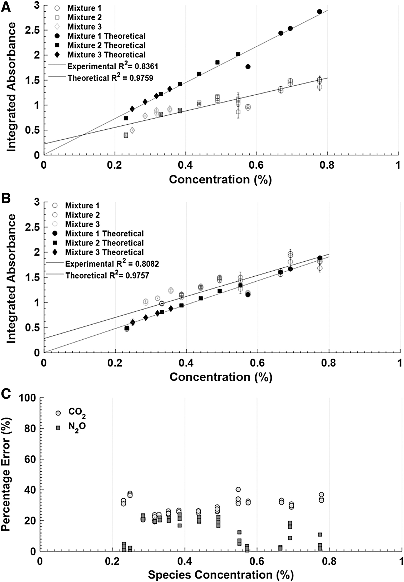
The integrated absorbance figures show that the system matches N₂O predictions much better than those for CO_2. For both species, correlation with the theoretical model increases as concentration decreases. The error bars showing the standard deviation at each concentration value indicate that the multiple tests exhibit less variance as both integrated absorbance values and concentration decrease. Using standard deviation curves for the absorbance with a 95% confidence interval (2-sigma standard deviation), the detection limit is defined as the point where the signal-to-noise ratio is equal to 1.⁵ Thus, the detection limit for CO₂ is determined to be 300 ppm, and the detection limit for N₂O is determined to be 220 ppm. In terms of CO₂-allowable limits, nominal spacecraft operations typically contain a maximum concentration of 5,000 ppm; during the Apollo 13 mission troubles, this concentration reached 20,000 ppm.¹⁶ In addition, humans may begin experiencing negative health risks when exposed to CO₂ concentrations of 5,000 ppm or higher; the average level within an enclosed room or home is typically 1,000 ppm.¹⁷ In terms of N₂O-allowable limits, there is as of yet no Occupational Safety and Health Administration exposure limit, but the recommended maximum exposure for humans within an 8-h workday is 50 ppm.¹⁸ While this is much lower than the current detection limit of the sensor, a lower minimum detection level could be achieved by the eventual use of more powerful LEDs with spectrum ranges more appropriate for N₂O.

The uncertainty in the integrated absorbance measurements is calculated by using the measured values to create logarithmic calibration curves and then quantifying the error due to uncertainty in relation to these equations. In general, for both species, the uncertainty increases as concentration increases due to the increase in variance. For CO₂, the uncertainty ranges between 7.9% and 13.8%; for N₂O, the values range between 5.4% and 11.3%.

Validation with Lasers

Laser experiments were performed with mixtures prepared in the same manner as those for the LED-based experiments; the concentrations are shown in Table 2.

Table 2.

Laser Validation Mixture Concentrations

Mixture	Percentage of CO₂	Percentage of N₂O	Percentage of N₂
1	0.355	0.356	99.29
2	0.674	0.654	98.67
3	0.518	0.503	98.97
4	0.537	0.521	98.94
5	0.201	0.195	99.60

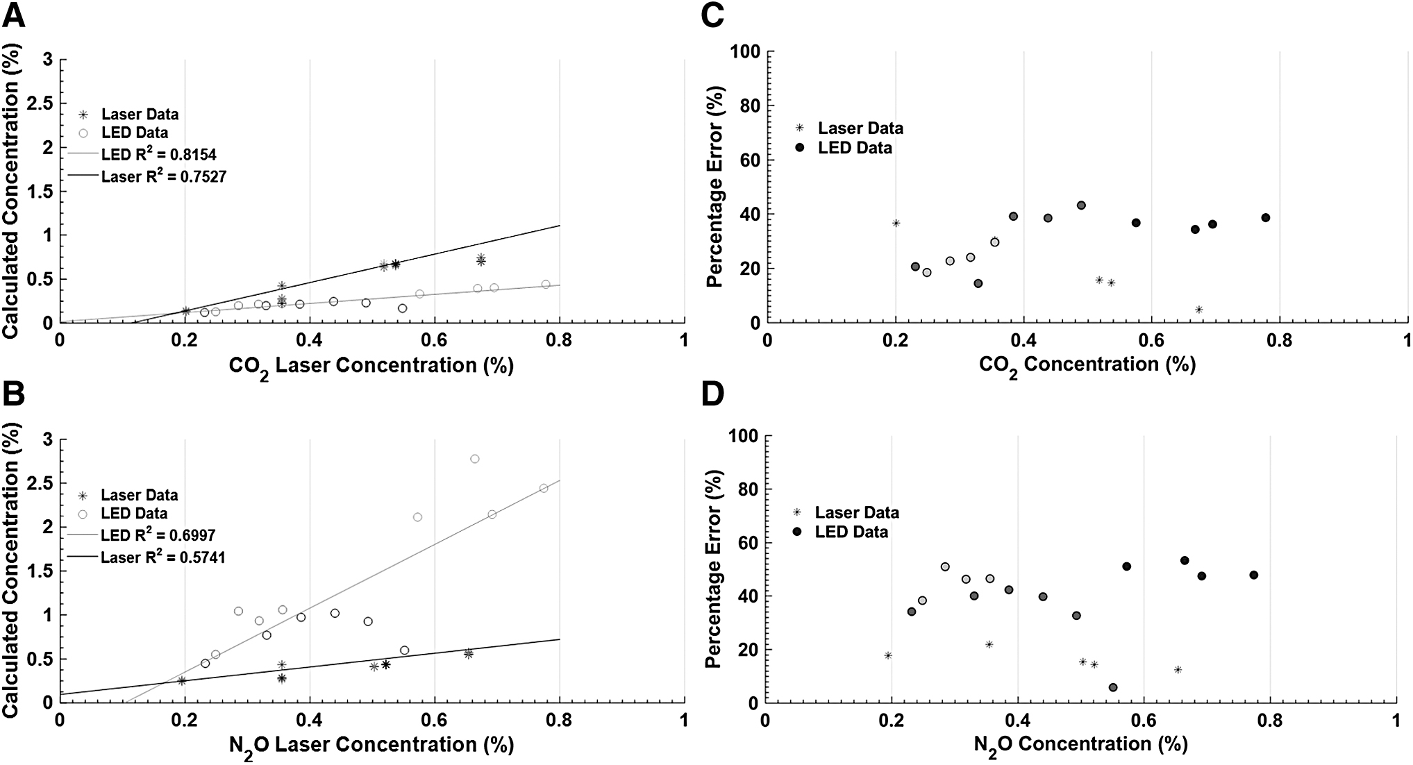
Figure 11 compares the calculated concentration data with similarly calculated concentration data from the LED experiments, again with the use of the Beer–Lambert law [Eq. (1)]. The laser intensities were recorded in terms of voltage, and the voltage levels were compared with those measured by the spectrum analyzer to ensure constant readings. Figure 11A shows the results for CO₂, and Figure 11B shows the results for N₂O; the LEDs interpolated absorbance data are used to find the point at a matching wavelength with the laser output. It is clear from the figure that the LED and laser values correlate better at lower concentrations. In general, the laser does much better at predicting the true relationship between the x- and y-axes than the LED. The CO₂ data for the LED, shown in Figure 11A, behave relatively as expected; it tends to predict the data better at lower concentrations than at higher values. The N₂O data, however, differ wildly. This is most likely because the N₂O laser is located at the end of the spectral range for the LED, and thus, the intensity is weaker in this region. Additionally, the laser is not located at the peak absorbance value detected by the LED. As a result, the method of looking at a single absorbance point for the LED and using this to calculate concentration results in a poorer fit for N₂O than for CO₂.

Fig. 11.

(A) CO₂ concentration for both the LED and laser experiments. (B) N₂O concentration for both the LED and laser experiments. The mixture concentration is shown along the x-axis, and the concentration calculated from intensity measurements is shown along the y-axis. (C) Percentage error for the CO₂ measurements for both the LED and laser. (D) Percentage error for the N₂O measurements for both the LED and laser.

The uncertainty in the calculated concentration measurements for the LEDs in Figure 11 is calculated by using the uncertainty values calculated earlier, for measured absorbance, and the Beer–Lambert law [Eq. (1)]. This results in a range of 9.2%–14.7% for CO₂ and 7.4%–12.4% for N₂O. For the lasers, the uncertainty is directly calculated through the Beer–Lambert law and results in average values of 7.3% for CO₂ and 6.1% for N₂O.

Summary and Future Work

An LED-based absorption spectroscopy sensor was developed and was proven functional for detecting CO₂ and N₂O in a laboratory environment. The grating design proves to be an effective method for using a single LED to detect multiple gases with absorption features at different wavelengths. While detection of both gases does not occur simultaneously, test time required for a full-range sweep can be ultimately reduced by optimizing wavelength range such that more tests are taken in a small range of interest and coarser measurements are taken elsewhere. Additionally, the technique of scanning across a wavelength range minimizes the potential for wavelength drift. This setup could also easily be expanded to include multiple LEDs centered at different wavelengths and ultimately expand the range of detectable gases. The successful testing in a laboratory fume hood introduces the potential for eventually using a similar setup to replace existing expensive and fragile sensor designs onboard space vehicles. As the complexities and costs associated with these basic safety measures deceases, the potential for commercial space travel increases.

Future work planned for this sensor includes increasing the wavelength test range while also decreasing the wavelength interval between test points. The eventual goal is to also test for other hazardous gases, such as CO. Additionally, this design should complete tests in harsher environments to further prove its capabilities.

Footnotes

Author Disclosure Statement

No competing financial interests exist.

Funding Information

Research at UCF was supported by financial assistance from the Federal Aviation Administration Center of Excellence for Commercial Space Transportation (FAA COE-CST), FAA Cooperative Agreement No. 15-C-CST-UCF-012, with Dr. Ken Davidian as program manager, Florida Space Institute (FSI), NASA Florida Space Grant Consortium (FSGC), the UCF Mechanical and Aerospace Department, and the UCF Office of Research and Commercialization.

References

Satish

, et al. Is CO2 an indoor pollutant? Direct effects of low-to-moderate CO2 concentrations on human decision-making performance. Environ Health Perspect. 2012; 120(12):1671–77.

Friedman

Risks and issues in fire safety on the space station. 1993. Presented at the Probabilistic Safety and Management Conference, San Diego, CA, 21–25 Mar. 1994.

Daues

K.R.

A history of spacecraft environmental control and life support systems. NASA Johnson Space Center; Houston, TX, United States. Preprint. 2006.

Teichert

, Fernholz

, Ebert

Simultaneous in situ measurement of CO, H 2 O, and gas temperatures in a full-sized coal-fired power plant by near-infrared diode lasers. Appl Opt. 2003; 42(12):2043–51.

Vurgaftman

, Meyer

, Ram-Mohan

High-power/low-threshold type-II interband cascade mid-IR laser-design and modeling. IEEE Photonics Technol Lett. 1997; 9(2):170–72.

Thurmond

, et al. A light-emitting diode-(LED-) based absorption sensor for simultaneous detection of carbon monoxide and carbon dioxide. Appl Spectrosc. 2016; 70(6):962–71.

Terracciano

, et al. Hazardous das detection sensor using broadband LED based absorption spectroscopy for space applications. New Space. 2018; 6(1):28–36.

Piatt

, Stutz

Differential Optical Absorption Spectroscopy, Principles and Applications. Heidelberg: Springer, 2008.

Rothman

L.S.

, et al. The HITRAN2012 molecular spectroscopic database. J Quantit Spectrosc Radiat Transf. 2013; 130:4–50.

10.

Palmer

C.A.

, Loewen

E.G.

Diffraction Grating Handbook. New York: Newport Corporation, 2005.

11.

Nickels

Memories of spaceshipone. Reinf Plastics, 2017; 61(2):83–86.

12.

Thorlabs. LED4300P -4200 nm LED with Parabolic Reflector, 10 μW Quasi-CW, 200 μW Pulsed, TO-18R. https://www.thorlabs.com/thorproduct.cfm?partnumber=LED4300P.

13.

Villar

M.S.

, et al. High-Altitude Balloon Flight Demonstration of LED-Based NDIR Multi-Gas Sensor for Space Applications, in AIAA SPACE and Astronautics Forum and Exposition. Orlando, FL: American Institute of Aeronautics and Astronautics, 2017.

14.

Thorlabs. Quantum Cascade Lasers (QCLs). https://www.thorlabs.com/newgrouppage9.cfm?objectgroup_id=6932 (Last accessed June 4, 2019).

15.

Yoo

, et al. Fast spatially resolved exhaust gas recirculation (EGR) distribution measurements in an internal combustion engine using absorption spectroscopy. Appl Spectrosc. 2015; 69(9):1047–1058.

16.

National Research

Council 2008

. Spacecraft Maximum Allowable Concentrations for Selected Airborne Contaminants: Volume 5. Washington

: The National Academies

Press

. https://doi.org/10.17226/12529 (Last accessed March 15, 2020).

17.

What Is the Allowable Level of Carbon Dioxide in an Occupied Space? https://www.ashrae.org/File Library/Technical Resources/Technical FAQs/TC-04.03-FAQ-35.pdf (Last accessed March 18, 2020).

18.

Henry

RJ.

Assessing environmental health concerns associated with nitrous oxide. J Am Dent Assoc. 1992; 123(12):41–47.