Bi-Modular Flow Characterization in Tissue Engineering Scaffolds Using Computational Fluid Dynamics and Particle Imaging Velocimetry

Abstract

As part of a tissue engineering (TE) therapy, cell-seeded scaffolds can be cultured in perfusion bioreactors in which the flow-mediated wall shear stress and the nutrient transport are factors that influence in vitro proliferation and osteogenic differentiation of the seeded progenitor cells. In this study both computational fluid dynamics simulations on idealized boundary conditions and circumstances and microparticle image velocimetry measurements on realistic conditions were carried out to quantify the fluid dynamic microenvironment inside a bone TE construct. The results showed that differences between actual and designed geometry and time-dependent character of the fluid flow caused a 19% difference in average fluid velocity and a 27% difference in wall shear stress between simulations and measurements. The computational fluid dynamics simulation enabled higher resolution and three-dimensional fluid flow quantification that could be quantitatively compared with a microparticle image velocimetry measurement. The coupling of numerical and experimental analysis provides a reliable and high-resolution bi-modular tool for quantifying the fluid dynamics that represent the basis to determine the relation between the hydrodynamic environment and cell growth and differentiation within TE scaffolds.

Introduction

In the last decades the tissue engineering (TE) field gained an increased interest for the repair of musculoskeletal tissue as an alternative to overcome complications related to tissue transplantation. Bone TE makes use of osteoprogenitor cells that are seeded into a suitable scaffold and cultured in a (perfusion) bioreactor, giving rise to a TE construct that is then implanted into the patient's bone defect site. Several requirements have been identified as fundamental for the in vitro production of three-dimensional (3D) tissues.¹ One of these factors is the creation of a flow environment that will in turn influence the biochemical and biophysical (such as mechanical) stimuli to which cells are exposed. On the one hand, determining the oxygen and nutrient distribution inside a bioreactor is a first step for overcoming mass transfer limitations that can otherwise lead to inhomogeneous cell and tissue growth and for establishing appropriate levels of oxygen and nutrients.² On the other hand, it is known that excessive fluid-flow-induced shear stress inside scaffolds can prevent cell attachment and hinder proliferation.³ Various studies showed that within a certain range fluid-flow-induced shear stress is responsible for modulating cell physiology and has a strong impact on tissue formation.^4–12 The optimal level of shear stress reported in these studies ranges between 0.05 mPa and 1 Pa depending not only on the cell type and the desired biological response. Wang and Tarbell found that when the same shear stress that was calculated to be present in a 3D scaffold was applied on the same cell type on a two-dimensional (2D) substrate, the production of prostaglandin was 10 times higher in 2D than in 3D.⁴ This illustrates that shear-stress-related cell response in 3D scaffolds cannot simply be deduced from 2D experiments and that it is important to accurately quantify not only the average but also the local distribution of shear stress in 3D scaffolds. There can be a considerable variance in shear stress within one scaffold. Boschetti et al. found in their model of a porous scaffold that the maximum local shear stress of scaffolds was up to 10 times the average value.¹³ Even in a scaffold for which the maximum shear stress was only 2.5–4.1 times the average, Vossenberg et al. found a higher cell density at the scaffold sites with the lowest local shear stress.¹⁴

In the last years different bioreactors were implemented both to allow perfusion of the culture medium and to provide flow-mediated mechanical stimuli that directly influence cell behavior.^15–18 The quantification of the nutrient supply and of the mechanical stimuli, both directly related to the medium fluid flow, is a key factor for the generation of bone tissue. To achieve this goal a number of studies have been performed using computational fluid dynamics (CFD)^19–26 or flow measurements techniques.^21,27

Different porous, macroscale, and microscale CFD models have been implemented to determine the shear stress distribution and the oxygen distribution inside TE constructs.^28–30 CFD simulations represent a powerful tool for describing the 3D cellular microenvironment, but they may present some limitations, depending on the simplifications of reality introduced when creating such models. Therefore, CFD models should be in conjunction with experimental validation when addressing questions such as scaffold optimization and bioreactor design.³¹

Since its introduction in 1998,³² microparticle imaging velocimetry (μ-PIV) has been applied by many researchers interested in fluid dynamics in microfluidic devices. μ-PIV can be used to quantify dynamic fluid flow at a sample rate up to 10 frames/s.³³ This technique has been improved, but more advanced techniques generally are less flexible and require more constraints. Three-dimensional velocity vectors at different depths have been determined using stereoscopic μ-PIV, but because this requires fluorescent particles, the maximum speed was limited to 10 nm/s.³⁴ Using a confocal microscope in combination with a pulsed laser, fluid velocity up to 0.5 mm/s is measurable.³⁵ This is until now limited to materials that are transparent, like polydimethylsiloxane, which was used by Provin et al. for μ-PIV measurements on a 330 μm high scaffold.³⁶ The majority of TE scaffolds made of ceramics and metals, however, are not transparent.

The objective of this study was to reliably and accurately quantify the spatial and temporal flow characteristics of the fluid flow inside a nontransparent bone TE scaffold using a bi-modular approach of modeling (CFD) and experiments (μ-PIV). The optical flow (OF)-based 2D μ-PIV technique was chosen instead of complicated high-end 3D systems to show how μ-PIV could be used in TE for fluid dynamics analysis inside a scaffold, without using specialized equipment and a steep learning curve. First, both CFD and μ-PIV were evaluated on a parallel plate bioreactor setup. Second, an analysis of the velocity field inside a scaffold was obtained by both techniques and a quantitative comparison was done.

Materials and Methods

2D+ concept

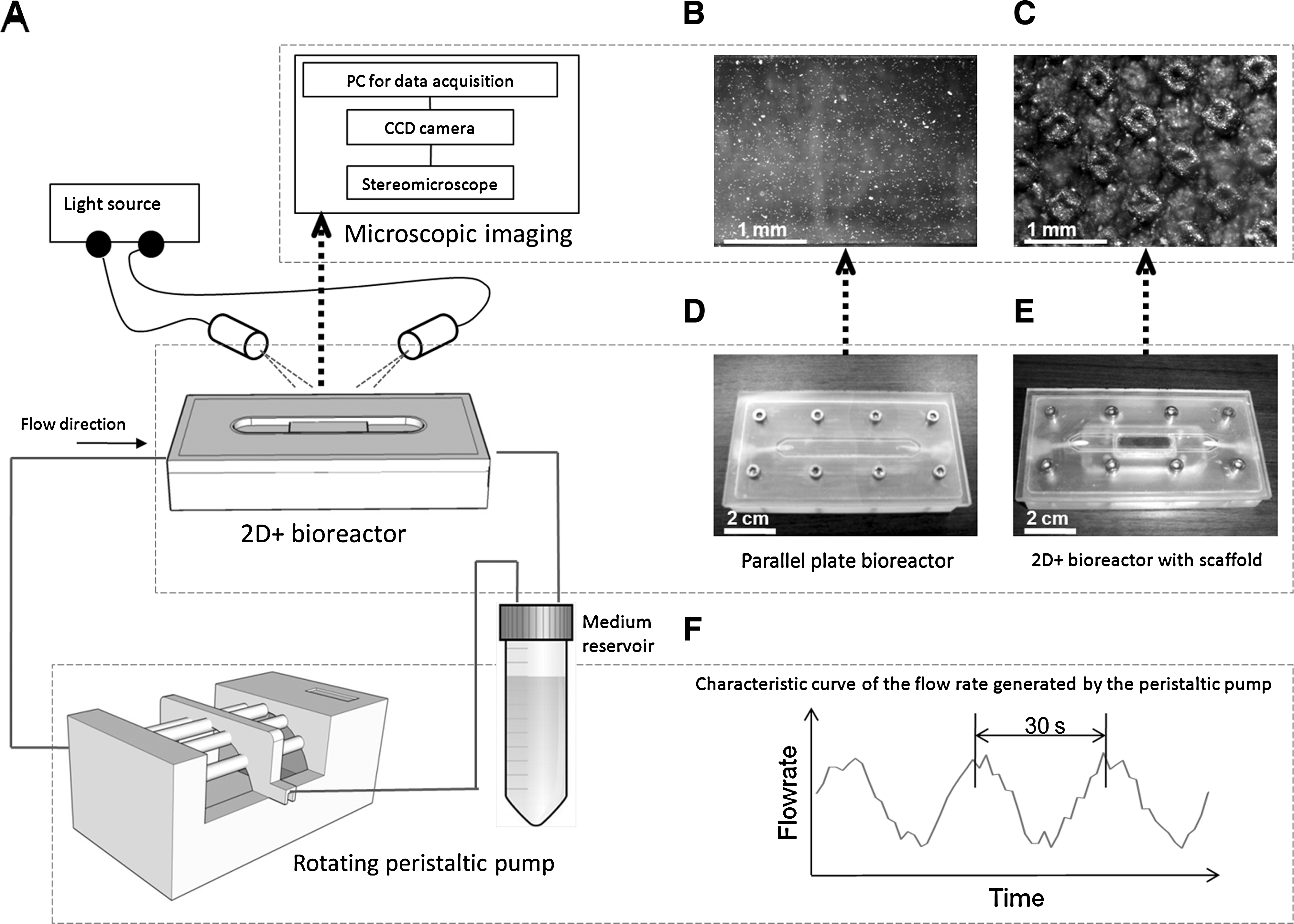
To realize observation of the fluid flow inside the nontransparent scaffold, a 2D+ concept was introduced in this study. The 2D+ bioreactor and scaffold represented a one geometrical unit cell high version of a full rapid prototyped 3D scaffold. As the 2D+ scaffold morphological and surface properties needed to resemble that of the 3D version, it also had to be produced in a similar way as the 3D scaffolds. The titanium alloy (Ti6Al4V) scaffold was produced by selective laser melting. Because scaffolds with similar material properties have been shown to enhance the growth of bone marrow stromal cells under perfusion, it makes them a suitable candidate for bone TE.³⁷ The parallel plate bioreactor, used for validation of the μ-PIV measurements, is shown in Figure 1D. The 2D+ bioreactor that was used to quantify the fluid flow inside the 2D+ scaffold is shown in Figure 1E.

FIG. 1.

(A) Scheme of the closed perfusion system used for μ-PIV experiments and CFD simulations consisting of a reservoir, a peristaltic pump (IPC-N; Ismatec SA), and a bioreactor all connected by tubing. (B) Representative image of the parallel plate bioreactor taken by the microscopic imaging system during experiments. (C) Representative image of the 2D+ bioreactor with scaffold taken by the microscopic imaging system during experiments. The 2D+ scaffold design is shown in Figure 2A. (D) Parallel plate bioreactor. The flow volume (50 × 6 × 0.5 mm) was created by using a transparent plate that covers the base plate using an O-ring and eight screws and was foreseen with an in- and outlet at the base plate. (E) 2D+ bioreactor containing a scaffold: similar to the parallel plate bioreactor, but with a void (20 × 6 × 0.5 mm) in the base plate that can contain a scaffold. (F) Peristaltic pump characteristic flow rate curve (illustration, not based on real data). CFD, computational fluid dynamics; μ-PIV, microparticle imaging velocimetry; 2D, two-dimensional.

CFD simulations

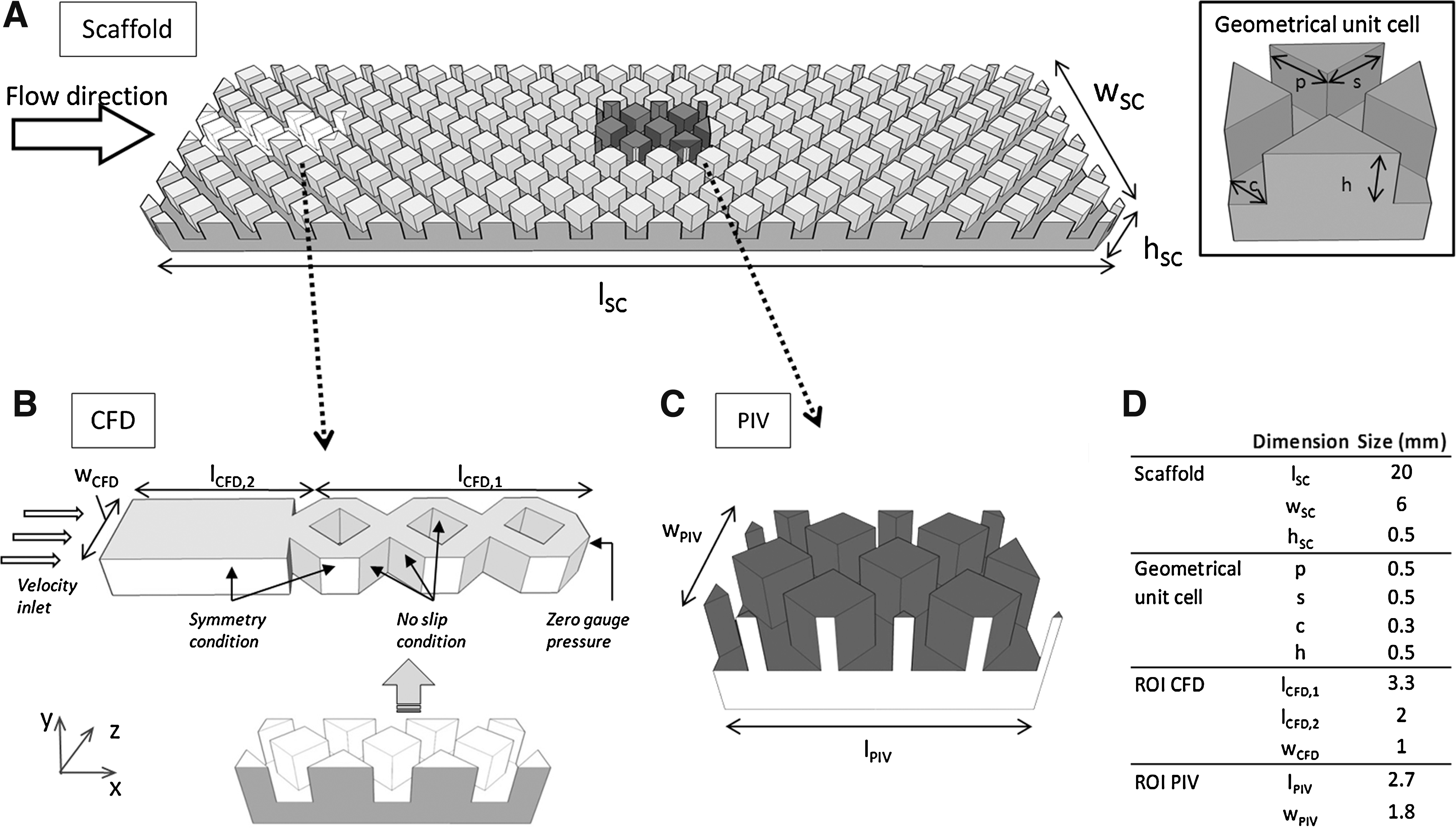
A CFD model was developed to predict the fluid velocity distribution and the wall shear stress (WSS). The ACIS-based solid modeler Gambit 2.2 (Fluent) was used to build the 3D model and the mesh, and the commercially available finite volume code Fluent 6.3 (Fluent) was used to set up and solve the problem. Due to the symmetry and the repeatability of the scaffold geometry (Fig. 2A), the domain was limited to one geometrical unit cell in width and three in length (Fig. 2B). The mesh was progressively refined through mesh sensitivity analysis until reaching convergence of the calculated velocity and WSS values (error below 1%). The final mesh presented 500,839 tetrahedral elements with an average edge length of 30 μm. The culture medium was regarded as an incompressible and homogeneous Newtonian fluid with a viscosity of 10⁻³ Pa · s and a density of 10³ kg/m³. A constant velocity of 0.1 mm/s was assigned to the inlet, corresponding to a flow rate of 0.018 mL/min or a pore volume refreshment rate of 0.5 min⁻¹ for this scaffold design. A zero-gauge pressure was applied to the outlet, a symmetry condition to the lateral surfaces, and a no slip condition to the walls of the structure. Steady-state Navier–Stokes equations were used to describe the flow problem.

FIG. 2.

(A) Design and dimensions of the 2D+ scaffold and its geometrical unit cell (inset), showing the ROI for μ-PIV in dark gray and for CFD in white. (B) ROI (bottom) and corresponding fluid domain (top) used for CFD, including an indication of the boundary conditions. Reference coordinate system used to represent fluid velocity components is displayed as well (C) ROI used for μ-PIV. (D) Overview of the dimensions. ROI, region of interest.

Experimental installation

To observe the fluid flow, the bioreactor was placed under a stereomicroscope (SteREO Discovery.V8; Carl Zeiss MicroImaging, Inc.). At a magnification of 3.2 × , the depth of focus of the objective lens was half of the scaffold height. The focus plane was manually set at 2/3 of the scaffold height to have the upper half of the flow volume in focus. For this 2D+ geometry, the flow in the upper half of the volume was assumed to be symmetrical to the bottom half and therefore representative for the entire height. The images were captured with a cooled charge-coupled device camera (SPOT Insight 2MP Firewire Colour Mosaic camera; Diagnostic Instruments Inc.) at a frame rate of 10 fps. To increase brightness 2 × 2 pixel binning was used to create 16 bit grayscale images of 600 × 800 pixels. Two gooseneck light spots were placed perpendicular to each other. Both spots were inclined at an angle of 10° to the bottom plane of the flow volume to reduce the direct reflection of the titanium scaffold and increase the contrast of the particles caused by light reflection. An overall view of this setup is shown in Figure 1A.

μ-PIV experiments

Before each experiment, all bioreactor parts and the scaffold were cleaned with demineralized water and household detergent in a sonic bath for 10 min, rinsed with distilled water, and dried. The scaffold was subsequently inserted in the base block void and the bioreactor was closed and checked for leakage. The medium reservoir was filled with distilled water containing opaque polyamide particles (Dantec Dynamics) with an average diameter of 20 μm and a density of 1.03 g/cm³. The perfusion loop parts were connected and the pump was activated. Once all air bubbles were removed from the perfusion loop, a flow rate of 0.018 mL/min was maintained constant for 10 min to make sure that a steady-state flow regime was obtained. Eventually, a 40 s image capturing sequence was performed, which was sufficiently long to cover one characteristic pump flow period (Fig. 1F).

Image processing

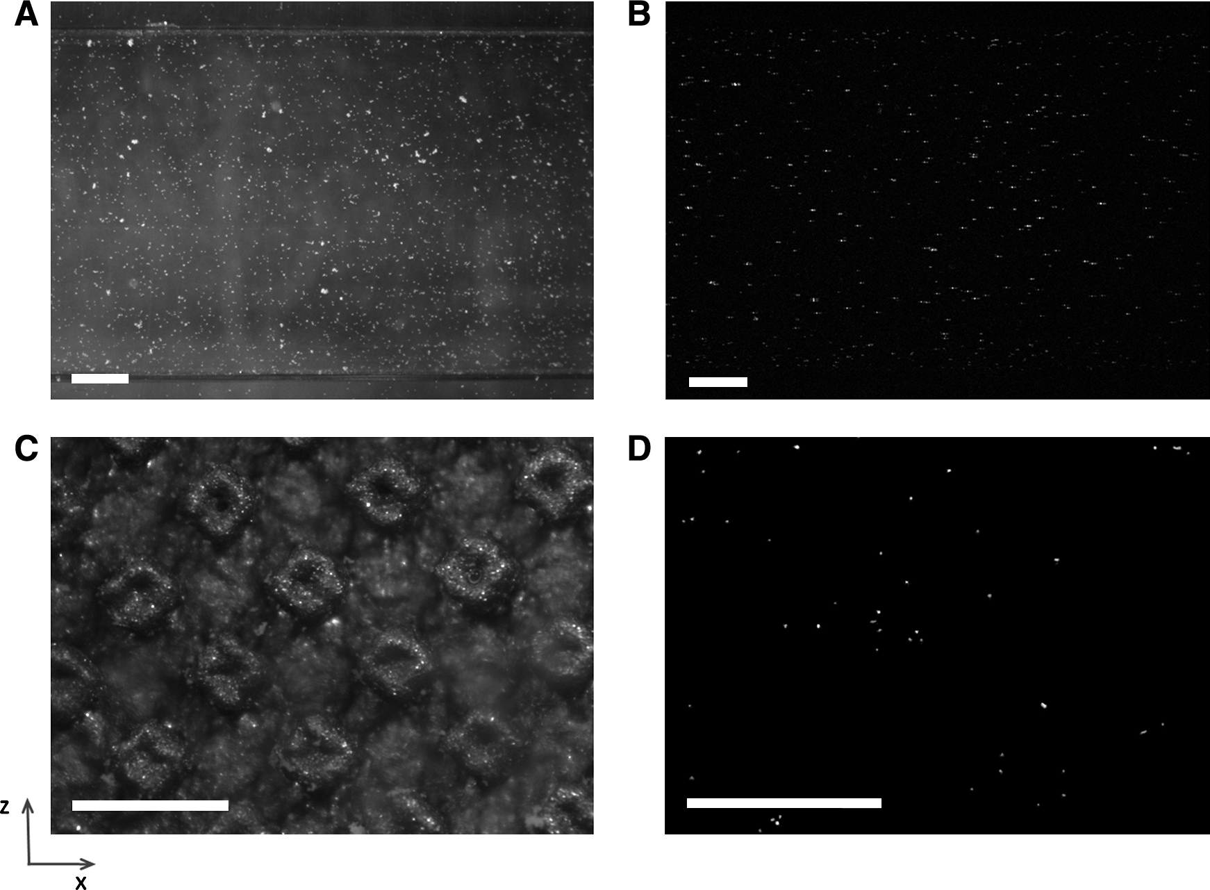
All image processing was done using Matlab (The Mathworks, Inc.). The representative image of the scaffold shown in Figure 3C illustrates the heterogeneous intensity of the background, which is caused by the reflection of light on the rough and highly reflective titanium surface. This makes it difficult to distinguish the particles from the background in a single image. To overcome this effect a background subtraction was done, to get images of the gray value texture of the moving particles on a black background. Examples of images of the parallel plate bioreactor and the bioreactor containing the scaffold before and after image processing are shown in Figure 3.

FIG. 3.

Image processing was done in Matlab as follows: for image 11 until 389 of the image sequence, the average of the gray values of previous 10 and the following 10 images in the sequence was taken to reconstruct the background. This was subtracted from the original image, increasing the contrast of the moving particles. Small particles and random noise were filtered out using a 3 × 3 size average filter. The image was then binarised, using a gray value threshold, to make the particles white and the background black. This image was used as a mask on the original image to retrieve the gray value information of the moving particles, which allows more accurate μ-PIV calculations. Representative example of a picture of the parallel plate and the 2D+ scaffold before (A, C) and after (B, D) image processing. Scale bar length = 1 mm.

OF algorithm

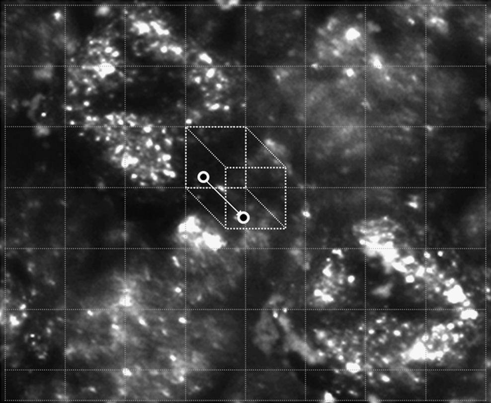
To quantify the flow from the processed image sequences, an OF algorithm was developed in Matlab. In this Lucas-Kanade-based OF algorithm, the velocity in the x and z direction of a particle in between two subsequent images is measured by searching for a (small) image region around the particle that is most similar to an equally sized region around the particle in the previous image (Fig. 4).³⁸ For this study 16 × 16 pixel regions were the smallest regions for which the algorithm performed well. For an image size of 600 × 800 pixels a 37 × 50 grid of velocity vectors could be measured, but only a 27 × 37 grid was used for further analysis to prevent possible inaccuracy at the image edges. For this 27 × 37 grid the velocity vectors were calculated for every two subsequent images.

FIG. 4.

Schematic representation of the Lucas–Kanade optical flow algorithm, measuring the displacement (= flow) of a particle in between two subsequent images by searching for a (small) image region around the particle that is most similar to an equally sized region around the particle in the previous image.

Statistical analysis

Statistical analyses were performed using one-way analysis of variance.

Results

Fluid flow in the parallel plate setup

Velocity as function of height: \documentclass{aastex}\usepackage{amsbsy}\usepackage{amsfonts}\usepackage{amssymb}\usepackage{bm}\usepackage{mathrsfs}\usepackage{pifont}\usepackage{stmaryrd}\usepackage{textcomp}\usepackage{portland, xspace}\usepackage{amsmath, amsxtra}\pagestyle{empty}\DeclareMathSizes{10}{9}{7}{6}\begin{document}$${\overline V}_{x} (Y)$$\end{document}

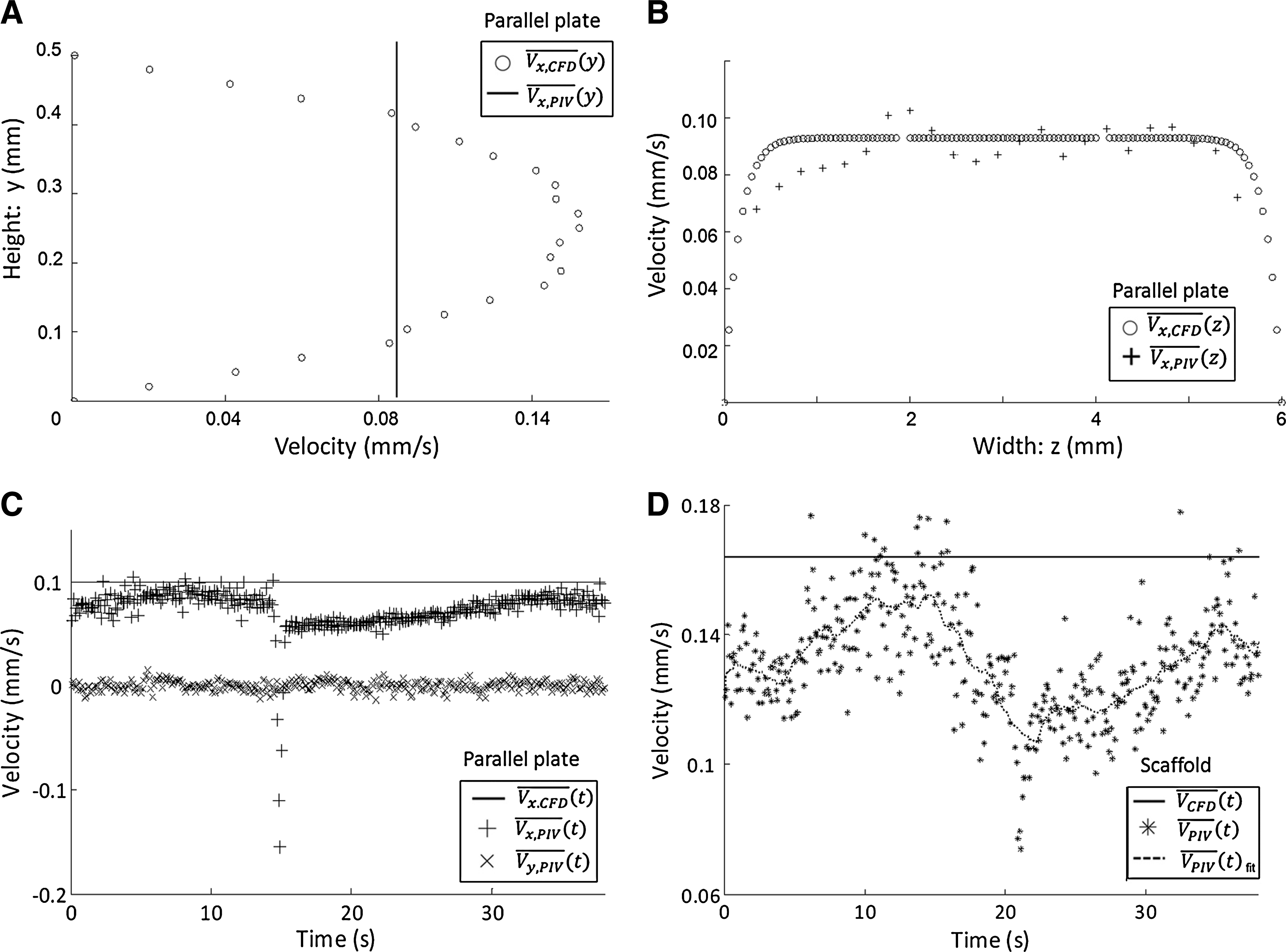
In the parallel plate setup, \documentclass{aastex}\usepackage{amsbsy}\usepackage{amsfonts}\usepackage{amssymb}\usepackage{bm}\usepackage{mathrsfs}\usepackage{pifont}\usepackage{stmaryrd}\usepackage{textcomp}\usepackage{portland, xspace}\usepackage{amsmath, amsxtra}\pagestyle{empty}\DeclareMathSizes{10}{9}{7}{6}\begin{document}$$\overline{V_{x, CFD}} (y)$$\end{document} , the velocity simulated with CFD in the flow direction averaged over width as function of the height, follows a parabolic velocity profile (Fig. 5A). The average of the velocity in the flow direction, given by the CFD simulation, \documentclass{aastex}\usepackage{amsbsy}\usepackage{amsfonts}\usepackage{amssymb}\usepackage{bm}\usepackage{mathrsfs}\usepackage{pifont}\usepackage{stmaryrd}\usepackage{textcomp}\usepackage{portland, xspace}\usepackage{amsmath, amsxtra}\pagestyle{empty}\DeclareMathSizes{10}{9}{7}{6}\begin{document}$$\overline{V_{x, CFD}}$$\end{document} is 0.087 mm/s. A similar parabolic profile cannot be measured with the μ-PIV measurement system, because this uses only 2D information. The average velocity in the flow direction, \documentclass{aastex}\usepackage{amsbsy}\usepackage{amsfonts}\usepackage{amssymb}\usepackage{bm}\usepackage{mathrsfs}\usepackage{pifont}\usepackage{stmaryrd}\usepackage{textcomp}\usepackage{portland, xspace}\usepackage{amsmath, amsxtra}\pagestyle{empty}\DeclareMathSizes{10}{9}{7}{6}\begin{document}$$\overline{V_{x, PIV}}$$\end{document} is therefore shown in Figure 5A as a vertical line and amounts to 0.083 mm/s, which is only 4.6% different from the value obtained by CFD.

FIG. 5.

(A) Modeled average velocity as a function of height in the parallel plate bioreactor, \documentclass{aastex}\usepackage{amsbsy}\usepackage{amsfonts}\usepackage{amssymb}\usepackage{bm}\usepackage{mathrsfs}\usepackage{pifont}\usepackage{stmaryrd}\usepackage{textcomp}\usepackage{portland, xspace}\usepackage{amsmath, amsxtra}\pagestyle{empty}\DeclareMathSizes{10}{9}{7}{6}\begin{document}$$\overline{{\rm V}_{\rm x, CFD}} {\rm (y)}$$\end{document} . The corresponding velocity measured with μ-PIV averaged over the 40 s period, \documentclass{aastex}\usepackage{amsbsy}\usepackage{amsfonts}\usepackage{amssymb}\usepackage{bm}\usepackage{mathrsfs}\usepackage{pifont}\usepackage{stmaryrd}\usepackage{textcomp}\usepackage{portland, xspace}\usepackage{amsmath, amsxtra}\pagestyle{empty}\DeclareMathSizes{10}{9}{7}{6}\begin{document}$$\overline{{\rm V}_{\rm x, PIV}} {\rm (y)}$$\end{document} , and is indicated with a vertical line. (B) Modeled and measured average velocity as a function of the width of the parallel plate bioreactor, \documentclass{aastex}\usepackage{amsbsy}\usepackage{amsfonts}\usepackage{amssymb}\usepackage{bm}\usepackage{mathrsfs}\usepackage{pifont}\usepackage{stmaryrd}\usepackage{textcomp}\usepackage{portland, xspace}\usepackage{amsmath, amsxtra}\pagestyle{empty}\DeclareMathSizes{10}{9}{7}{6}\begin{document}$$\overline{{\rm V}_{\rm x, CFD}} {\rm (z)}$$\end{document} and \documentclass{aastex}\usepackage{amsbsy}\usepackage{amsfonts}\usepackage{amssymb}\usepackage{bm}\usepackage{mathrsfs}\usepackage{pifont}\usepackage{stmaryrd}\usepackage{textcomp}\usepackage{portland, xspace}\usepackage{amsmath, amsxtra}\pagestyle{empty}\DeclareMathSizes{10}{9}{7}{6}\begin{document}$$\overline{{\rm V}_{\rm x, PIV}} {\rm (z)}$$\end{document} for the two techniques. (C) Measured average of the x and y components of the velocity in the parallel plate bioreactor as a function of time, \documentclass{aastex}\usepackage{amsbsy}\usepackage{amsfonts}\usepackage{amssymb}\usepackage{bm}\usepackage{mathrsfs}\usepackage{pifont}\usepackage{stmaryrd}\usepackage{textcomp}\usepackage{portland, xspace}\usepackage{amsmath, amsxtra}\pagestyle{empty}\DeclareMathSizes{10}{9}{7}{6}\begin{document}$$\overline{{\rm V}_{\rm x, PIV}} {\rm (t)}$$\end{document} and \documentclass{aastex}\usepackage{amsbsy}\usepackage{amsfonts}\usepackage{amssymb}\usepackage{bm}\usepackage{mathrsfs}\usepackage{pifont}\usepackage{stmaryrd}\usepackage{textcomp}\usepackage{portland, xspace}\usepackage{amsmath, amsxtra}\pagestyle{empty}\DeclareMathSizes{10}{9}{7}{6}\begin{document}$$\overline{{\rm V}_{\rm y, PIV}} {\rm (t)}$$\end{document} . The inlet velocity used for the CFD simulations is indicated with a horizontal line \documentclass{aastex}\usepackage{amsbsy}\usepackage{amsfonts}\usepackage{amssymb}\usepackage{bm}\usepackage{mathrsfs}\usepackage{pifont}\usepackage{stmaryrd}\usepackage{textcomp}\usepackage{portland, xspace}\usepackage{amsmath, amsxtra}\pagestyle{empty}\DeclareMathSizes{10}{9}{7}{6}\begin{document}$$\overline{{\rm V}_{\rm x, CFD}} {\rm (t)}$$\end{document} . (D) Similar graph as (C) for the bioreactor containing the scaffold.

Velocity as function of width: \documentclass{aastex}\usepackage{amsbsy}\usepackage{amsfonts}\usepackage{amssymb}\usepackage{bm}\usepackage{mathrsfs}\usepackage{pifont}\usepackage{stmaryrd}\usepackage{textcomp}\usepackage{portland, xspace}\usepackage{amsmath, amsxtra}\pagestyle{empty}\DeclareMathSizes{10}{9}{7}{6}\begin{document}$${\overline V}_{x} (Z)$$\end{document}

Velocity as a function of time V(t)

For the μ-PIV measurements, a 2D velocity vector grid is calculated every 0.1 s. For every time point t, the average x component of the velocity of all the grid points in the image was calculated, which was symbolized as \documentclass{aastex}\usepackage{amsbsy}\usepackage{amsfonts}\usepackage{amssymb}\usepackage{bm}\usepackage{mathrsfs}\usepackage{pifont}\usepackage{stmaryrd}\usepackage{textcomp}\usepackage{portland, xspace}\usepackage{amsmath, amsxtra}\pagestyle{empty}\DeclareMathSizes{10}{9}{7}{6}\begin{document}$$\overline{V_{x , PIV}} (t)$$\end{document} . Figure 5C shows that \documentclass{aastex}\usepackage{amsbsy}\usepackage{amsfonts}\usepackage{amssymb}\usepackage{bm}\usepackage{mathrsfs}\usepackage{pifont}\usepackage{stmaryrd}\usepackage{textcomp}\usepackage{portland, xspace}\usepackage{amsmath, amsxtra}\pagestyle{empty}\DeclareMathSizes{10}{9}{7}{6}\begin{document}$$\overline{V_{x , PIV}} (t)$$\end{document} inside the parallel plate bioreactor is not constant in time, but that there is a short reversed flow. \documentclass{aastex}\usepackage{amsbsy}\usepackage{amsfonts}\usepackage{amssymb}\usepackage{bm}\usepackage{mathrsfs}\usepackage{pifont}\usepackage{stmaryrd}\usepackage{textcomp}\usepackage{portland, xspace}\usepackage{amsmath, amsxtra}\pagestyle{empty}\DeclareMathSizes{10}{9}{7}{6}\begin{document}$$\overline{V_{x , PIV}} (t)$$\end{document} drops from 0.09 to −0.15 mm/s and then increases again to 0.05 mm/s within a time interval of 0.5 s (Fig. 5C). After this, \documentclass{aastex}\usepackage{amsbsy}\usepackage{amsfonts}\usepackage{amssymb}\usepackage{bm}\usepackage{mathrsfs}\usepackage{pifont}\usepackage{stmaryrd}\usepackage{textcomp}\usepackage{portland, xspace}\usepackage{amsmath, amsxtra}\pagestyle{empty}\DeclareMathSizes{10}{9}{7}{6}\begin{document}$$\overline{V_{x , PIV}} (t)$$\end{document} rises slowly to 0.09 mm/s during the next 30 s, after which there is again a reversed flow and the rest of the cycle is repeated. This 30 s period corresponds to the transition between two subsequent steel rollers in the peristaltic pump. The constant \documentclass{aastex}\usepackage{amsbsy}\usepackage{amsfonts}\usepackage{amssymb}\usepackage{bm}\usepackage{mathrsfs}\usepackage{pifont}\usepackage{stmaryrd}\usepackage{textcomp}\usepackage{portland, xspace}\usepackage{amsmath, amsxtra}\pagestyle{empty}\DeclareMathSizes{10}{9}{7}{6}\begin{document}$$\overline{V_{x , CFD}} (t)$$\end{document} is indicated in Figure 5C with a horizontal line at 0.1 mm/s, which is the uniform velocity in the x direction at the inlet cross section, used for the CFD simulation.

Fluid flow in the scaffold

Velocity as a function of time: V(t)

A periodic behavior can be noticed for the velocity in the 2D + bioreactor with scaffold as well. \documentclass{aastex}\usepackage{amsbsy}\usepackage{amsfonts}\usepackage{amssymb}\usepackage{bm}\usepackage{mathrsfs}\usepackage{pifont}\usepackage{stmaryrd}\usepackage{textcomp}\usepackage{portland, xspace}\usepackage{amsmath, amsxtra}\pagestyle{empty}\DeclareMathSizes{10}{9}{7}{6}\begin{document}$$\overline{V_{PIV}} (t)$$\end{document} fluctuates in a sine like way between 0.09 and 0.17 mm/s (Fig. 5D).

Velocity as a function of space: V(x, y, z)

The fluid flow in the scaffold predicted by the CFD simulation has a maximum velocity of 0.48 mm/s at the intersection of two channels (Fig. 6A). The velocity component in the y direction is zero. To make a quantitative comparison between the CFD and the μ-PIV results, the vector field of the irregular 3D CFD mesh was transformed to the regular 2D μ-PIV grid. This was done as follows: the scaffold volume was divided into equal rectangular prisms, centered at the 2D μ-PIV grid points. The velocity in every 2D grid point is calculated by taking the average velocity of all the 3D CFD grid points in the corresponding prismatic volume. Figure 6B shows the CFD vector field for one scaffold unit cell before (left) and after (right) this transformation. Because at the region of interest of the μ-PIV measurements (Fig. 2A) the flow is fully developed, the CFD simulated flow pattern is expected to be the same for every unit cell.

FIG. 6.

(A) A horizontal cross section at y = 0.25 mm of the 3D CFD simulation results for the 2D + scaffold. (B) Top view of the velocity vectors of a unit cell by CFD before (left) and after (right) transformation (averaging) from the mesh coordinates to the μ-PIV coordinates. Color images available online at www.liebertonline.com/ten.

In general, \documentclass{aastex}\usepackage{amsbsy}\usepackage{amsfonts}\usepackage{amssymb}\usepackage{bm}\usepackage{mathrsfs}\usepackage{pifont}\usepackage{stmaryrd}\usepackage{textcomp}\usepackage{portland, xspace}\usepackage{amsmath, amsxtra}\pagestyle{empty}\DeclareMathSizes{10}{9}{7}{6}\begin{document}$$\overline{V_{PIV}} (x, z)$$\end{document} and \documentclass{aastex}\usepackage{amsbsy}\usepackage{amsfonts}\usepackage{amssymb}\usepackage{bm}\usepackage{mathrsfs}\usepackage{pifont}\usepackage{stmaryrd}\usepackage{textcomp}\usepackage{portland, xspace}\usepackage{amsmath, amsxtra}\pagestyle{empty}\DeclareMathSizes{10}{9}{7}{6}\begin{document}$$\overline{V_{CFD}} (x, z)$$\end{document} inside the scaffold have the same three fluid flow characteristics: (1) in the channels the fluid flows parallel to the strut walls, (2) there is a narrow band of low velocity near the struts, and (3) there is a higher velocity in the central part of the channel. At the intersections the velocity is highest, and the flow direction gradually rotates with 90° to align to the direction of the next channel.

Although qualitatively both techniques display a similar flow field, there are several differences. Figure 7B shows that for the μ-PIV results the fluid flow follows the scaffold walls closely, which is not the case for the CFD results (Fig. 7A). The average channel width was measured on a scanning electron microscope image of the scaffold (data not shown) and was 0.371 mm, which is 17% higher than the designed width (0.3 mm). Because in reality the channels are wider than in the design, the average velocity in the scaffold is overestimated by the CFD simulation. \documentclass{aastex}\usepackage{amsbsy}\usepackage{amsfonts}\usepackage{amssymb}\usepackage{bm}\usepackage{mathrsfs}\usepackage{pifont}\usepackage{stmaryrd}\usepackage{textcomp}\usepackage{portland, xspace}\usepackage{amsmath, amsxtra}\pagestyle{empty}\DeclareMathSizes{10}{9}{7}{6}\begin{document}$$\overline{V_{PIV}} (x, z)$$\end{document} is 0.136 mm/s, while \documentclass{aastex}\usepackage{amsbsy}\usepackage{amsfonts}\usepackage{amssymb}\usepackage{bm}\usepackage{mathrsfs}\usepackage{pifont}\usepackage{stmaryrd}\usepackage{textcomp}\usepackage{portland, xspace}\usepackage{amsmath, amsxtra}\pagestyle{empty}\DeclareMathSizes{10}{9}{7}{6}\begin{document}$$\overline{V_{CFD}} (x, z)$$\end{document} amounts to 0.168 mm/s (19% difference).

FIG. 7.

Results and quantitative comparison of the 2D fluid flow pattern determined by CFD (after transformation) and μ-PIV. Velocity vectors determined by CFD (A, C) and μ-PIV (B, D) superimposed to a top view image of the scaffold (A, B) and to a contour plot of the velocity magnitude (C, D), respectively. (E) Contour plot of \documentclass{aastex}\usepackage{amsbsy}\usepackage{amsfonts}\usepackage{amssymb}\usepackage{bm}\usepackage{mathrsfs}\usepackage{pifont}\usepackage{stmaryrd}\usepackage{textcomp}\usepackage{portland, xspace}\usepackage{amsmath, amsxtra}\pagestyle{empty}\DeclareMathSizes{10}{9}{7}{6}\begin{document}$$[\overline{{\rm V}_{\rm CFD}} ({\rm x , z}) - \overline{{\rm V}_{\rm PIV}} ({\rm x , z})]$$\end{document} . (F) Velocity histogram of distribution of all 2D grid points of CFD and μ-PIV. Color images available online at www.liebertonline.com/ten.

A second phenomenon shown by the μ-PIV measurements is a nonzero flow over some parts of the struts. Contrary to what was assumed in the CFD simulations, the strut upper surface is not always in perfect contact with the cover plate, creating small voids that allow fluid flow. As a result of the wider channels and the voids between struts and cover plate, the area where there is no fluid flow is only 17.8% for the μ-PIV measurement as compared to 30.7% for the CFD simulation (Fig. 7F).

The contour plot of difference in velocity between the two techniques, \documentclass{aastex}\usepackage{amsbsy}\usepackage{amsfonts}\usepackage{amssymb}\usepackage{bm}\usepackage{mathrsfs}\usepackage{pifont}\usepackage{stmaryrd}\usepackage{textcomp}\usepackage{portland, xspace}\usepackage{amsmath, amsxtra}\pagestyle{empty}\DeclareMathSizes{10}{9}{7}{6}\begin{document}$$[\overline{V_{CFD}} (x, z) - \overline{V_{PIV}} (x, z)]$$\end{document} , shows that it is not random across the scaffold. In the center of the channels the difference is biggest (>0.2 mm/s), which means that the CFD velocity is higher (Fig. 7E). When moving from the center of the channels toward the struts, \documentclass{aastex}\usepackage{amsbsy}\usepackage{amsfonts}\usepackage{amssymb}\usepackage{bm}\usepackage{mathrsfs}\usepackage{pifont}\usepackage{stmaryrd}\usepackage{textcomp}\usepackage{portland, xspace}\usepackage{amsmath, amsxtra}\pagestyle{empty}\DeclareMathSizes{10}{9}{7}{6}\begin{document}$$[\overline{V_{CFD}} (x, z) - \overline{V_{PIV}} (x, z)]$$\end{document} becomes lower and it becomes negative near the strut walls, where \documentclass{aastex}\usepackage{amsbsy}\usepackage{amsfonts}\usepackage{amssymb}\usepackage{bm}\usepackage{mathrsfs}\usepackage{pifont}\usepackage{stmaryrd}\usepackage{textcomp}\usepackage{portland, xspace}\usepackage{amsmath, amsxtra}\pagestyle{empty}\DeclareMathSizes{10}{9}{7}{6}\begin{document}$$\overline{V_{CFD}} (x, z)$$\end{document} is lower than \documentclass{aastex}\usepackage{amsbsy}\usepackage{amsfonts}\usepackage{amssymb}\usepackage{bm}\usepackage{mathrsfs}\usepackage{pifont}\usepackage{stmaryrd}\usepackage{textcomp}\usepackage{portland, xspace}\usepackage{amsmath, amsxtra}\pagestyle{empty}\DeclareMathSizes{10}{9}{7}{6}\begin{document}$$\overline{V_{PIV}} (x, z)$$\end{document} .

Shear stress as function of space: \documentclass{aastex}\usepackage{amsbsy}\usepackage{amsfonts}\usepackage{amssymb}\usepackage{bm}\usepackage{mathrsfs}\usepackage{pifont}\usepackage{stmaryrd}\usepackage{textcomp}\usepackage{portland, xspace}\usepackage{amsmath, amsxtra}\pagestyle{empty}\DeclareMathSizes{10}{9}{7}{6}\begin{document}$$\overline{\tau} (\rm x, z)$$\end{document}

\documentclass{aastex}\usepackage{amsbsy}\usepackage{amsfonts}\usepackage{amssymb}\usepackage{bm}\usepackage{mathrsfs}\usepackage{pifont}\usepackage{stmaryrd}\usepackage{textcomp}\usepackage{portland, xspace}\usepackage{amsmath, amsxtra}\pagestyle{empty}\DeclareMathSizes{10}{9}{7}{6}\begin{document}$$\overline{\tau_{CFD}} (x, z)$$\end{document} and \documentclass{aastex}\usepackage{amsbsy}\usepackage{amsfonts}\usepackage{amssymb}\usepackage{bm}\usepackage{mathrsfs}\usepackage{pifont}\usepackage{stmaryrd}\usepackage{textcomp}\usepackage{portland, xspace}\usepackage{amsmath, amsxtra}\pagestyle{empty}\DeclareMathSizes{10}{9}{7}{6}\begin{document}$$\overline{\tau_{PIV}} (x, z)$$\end{document} were calculated from \documentclass{aastex}\usepackage{amsbsy}\usepackage{amsfonts}\usepackage{amssymb}\usepackage{bm}\usepackage{mathrsfs}\usepackage{pifont}\usepackage{stmaryrd}\usepackage{textcomp}\usepackage{portland, xspace}\usepackage{amsmath, amsxtra}\pagestyle{empty}\DeclareMathSizes{10}{9}{7}{6}\begin{document}$$\overline{V_{CFD}} (x, z)$$\end{document} and \documentclass{aastex}\usepackage{amsbsy}\usepackage{amsfonts}\usepackage{amssymb}\usepackage{bm}\usepackage{mathrsfs}\usepackage{pifont}\usepackage{stmaryrd}\usepackage{textcomp}\usepackage{portland, xspace}\usepackage{amsmath, amsxtra}\pagestyle{empty}\DeclareMathSizes{10}{9}{7}{6}\begin{document}$$\overline{V_{PIV}} (x, z)$$\end{document} and they have the following similarities: both have higher values at the strut walls than in the channels, and the highest shear stress values (5.1 and 4.8 mPa for CFD and μ-PIV, respectively) are located at the left and right corners of the struts (Fig. 8A, B). The average shear stress at the scaffold wall (WSS) equaled 2.4 mPa for μ-PIV measurements and 3.3 mPa for CFD simulations, respectively (27% difference). Figure 8D shows that the difference \documentclass{aastex}\usepackage{amsbsy}\usepackage{amsfonts}\usepackage{amssymb}\usepackage{bm}\usepackage{mathrsfs}\usepackage{pifont}\usepackage{stmaryrd}\usepackage{textcomp}\usepackage{portland, xspace}\usepackage{amsmath, amsxtra}\pagestyle{empty}\DeclareMathSizes{10}{9}{7}{6}\begin{document}$$[\overline{\tau_{CFD}} (x, z) - \overline{\tau_{PIV}} (x, z)]$$\end{document} has a pattern that follows the scaffold geometry. As a result of the difference in channel width some regions that were in the fluid domain for the μ-PIV measurements were in the scaffold domain for the CFD simulations. This means that the maximum local difference in shear stress calculated for the absolute coordinates, which was almost 100% of the average shear stress value, is not the true difference between simulated and measured WSS. At the same relative positions on the scaffold wall, the shear stress determined with μ-PIV is only between 5% and 50% lower than the CFD-simulated shear stress.

FIG. 8.

Results and quantitative comparison of the 2D shear stress pattern determined by CFD and μ-PIV. Contour plot of the shear stress determined by CFD (A) and μ-PIV (B). (C) Contour plot of the difference between the shear stress determined by CFD and μ-PIV \documentclass{aastex}\usepackage{amsbsy}\usepackage{amsfonts}\usepackage{amssymb}\usepackage{bm}\usepackage{mathrsfs}\usepackage{pifont}\usepackage{stmaryrd}\usepackage{textcomp}\usepackage{portland, xspace}\usepackage{amsmath, amsxtra}\pagestyle{empty}\DeclareMathSizes{10}{9}{7}{6}\begin{document}$$[\overline{\tau_{\rm CFD}} ({\rm x, z}) - \overline{\tau_{\rm PIV}} ({\rm x, z})]$$\end{document} for all grid points. (D) Histogram of shear stress distribution of all 2D grid points of CFD and μ-PIV. Color images available online at www.liebertonline.com/ten.

Discussion

In this study a bi-modular approach was used for a quantitative comparison of a CFD simulation for idealized geometrical and boundary conditions to a μ-PIV measurement for realistic conditions. The average velocity inside the 2D+ scaffold simulated with CFD was 19% higher than the measured velocity, and the average shear stress was 27% higher than the values obtained from the μ-PIV measurements. This work showed that there are two aspects of the difference between reality and idealized conditions in perfusion bioreactors: fluctuations in flow rate and scaffold geometry.

First, the μ-PIV measurements pointed out that the fluid flow in this particular setup is dynamic and cannot be regarded as constant in time. This is relevant information that illustrates the need for a good pump control in scaffold perfusion research, because previous studies showed that there is a difference between cellular behavior under constant versus dynamic flow conditions.³⁹ There was a less sudden change in flow rate in the scaffold compared to the parallel plate setup, and this was probably caused by the scaffold itself, which acts like a flow dampener owing to a reduced permeability, and making the system more inert to rapid changes in tube pressure.

Second, the differences in the designed scaffold geometry and the actual geometry after selective laser melting production had an important influence on the fluid flow pattern. The difference between the design of regular scaffolds and their actual geometry is a known property of rapid prototyped production techniques and has been quantified by others.⁴⁰ Williams et al., for instance, showed that actual porosity of their selective laser sintering produced polycaprolactone scaffolds was 30%–40% lower than the designed porosity. In our study, the scaffold channels were wider and the struts were thinner than in the design, which according to the work of Vossenberg et al. can have a mayor effect on the average and maximum shear stress values.¹⁴ To investigate the effect of channel width for the 2D+ scaffold, an additional CFD analysis was performed that took into account the actual width (0.371 mm instead of 0.3 mm, as mentioned before). Average velocity and WSS were no longer significantly different from the μ-PIV calculations and the average error between CFD and μ-PIV was reduced by 25%.

Another geometrical difference of the scaffold was that the corners of the struts were round instead of sharp and that at certain struts fluid could flow between the top of the scaffold and the cover plate of the bioreactor. Although the surface areas of these regions are smaller than the total surface area, the difference in microenvironment could locally cause the cells to respond differently, thereby influencing the experimental results.

Many studies have shown that shear stress and nutrient concentrations have an important influence on cell response, but the reported critical shear stress and nutrient concentration levels vary and are difficult to compare because of the difference in cell types, scaffolds, and cell culture methods. It is not known if the differences in velocity and shear stress that were found in this study are big enough to influence the outcome of biological experiments performed on this perfusion system. However, it can be concluded that a linear scaffold design and production process, entirely based on computer models, can lead to scaffolds that do not provide the predicted microenvironment and desired cell behavior. Modeling methods like CFD are powerful tools for TE, but to be reliable and accurate they should be part of an iterative approach where the models are continuously improved by feedback from physical experiments. μ-PIV is a suitable technique for such a bi-modular approach with CFD simulations, but was until now limited to transparent materials.³⁶ The 2D+ concept that was developed here provided a methodology for more challenging materials and wide variety of scaffold types.

To conclude, new directions for future quantification of the fluid flow inside scaffolds are illustrated in a scheme with four different approaches in Figure 9. Instead of using the designed geometry (Fig. 9, approach I), the actual geometry of the scaffold after production can be used for CFD analysis (Fig. 9, approach II). For irregular scaffolds this has already been done. In 2002 Raimondi et al. used light microscopic images of scaffold sections to do 2D CFD analysis of a fibrous scaffold.⁴² For a 3D measurement of the scaffold geometry, microcomputed tomography has been used for scaffolds made of different materials, like polylactic acid–calcium phosphate glass scaffolds,⁴³ titanium and hydroxy-apatite,⁴⁴ polyestherurethane foam,²³ and poly(ethylene glycol terephthalate) (PEGT)/poly(butylene terephthalate) (PBT).²⁸ For regular scaffolds this has not been done yet. The bi-modular approach (Fig. 9, approach III) that was used here provides an even higher reliability, because differences between the idealized circumstances and reality other than scaffold geometry can be quantified by comparing fluid flow simulations with measurements. Approaches II and III both require a physical scaffold. This, however, is not satisfactory for researchers who are interested in knowing the fluid flow inside the scaffold in the design phase, before the actual production. Boschetti et al., for example, investigated the effect of pore size on local fluid flow and WSS,¹³ and Olivares et al. proposed a gradient in pore sizes to trigger a gradient in differentiation, based on differences in fluid flow properties.⁴⁵ The production and measurement of such a range of scaffold designs would be costly and time consuming. A different approach IV (Fig. 9) is needed where the difference between the design and the geometry is simulated. This requires innovative models that do not exist today but are seemingly possible to make. The simulated geometry should then be used for CFD** analysis instead of the designed geometry.

FIG. 9.

Overview of approaches to quantify the fluid dynamic environment in tissue engineering scaffolds. In approach I, CFD based on the scaffold design is used as a stand-alone technique. Approach II uses the actual scaffold geometry instead of the designed geometry to perform a more accurate CFD* analysis. Approach III is the bi-modular approach used in this study, in which the CFD analysis is used together with μ-PIV measurements on the actual system. Approach IV is a new concept where the scaffold does not have to be produced. Instead, the CFD** analysis is done on a computer simulation of the scaffold geometry after production.

Footnotes

Acknowledgments

This work is part of Prometheus, the Leuven Research & Development Division of Skeletal Tissue Engineering of the Katholieke Universiteit Leuven.

Disclosure Statement

No competing financial interests exist.

References

Mikos

A.G.

, Herring

S.W.

, Ochareon

, Elisseeff

, Lu

H.H.

, Kandel

et al. Engineering complex tissues. Tissue Eng, 12:3307. 2006.

Malda

, Klein

T.J.

, Upton

The roles of hypoxia in the in vitro engineering of tissues. Tissue Eng, 13:2153. 2007.

Martin

, Vermette

Bioreactors for tissue mass culture: design, characterization, and recent advances. Biomaterials, 26:7481. 2005.

Wang

, Tarbell

J.M.

Effect of fluid flow on smooth muscle cells in a 3-dimensional collagen gel model. Arterioscler Thromb Vasc Biol, 20:2220. 2000.

Sikavitsas

V.I.

, Bancroft

G.N.

, Holtorf

H.L.

, Jansen

J.A.

, Mikos

A.G.

Mineralized matrix deposition by marrow stromal osteoblasts in 3D perfusion culture increases with increasing fluid shear forces. Proc Natl Acad Sci U S A, 100:14683. 2003.

Gutierrez

R.A.

, Crumpler

E.T.

Potential effect of geometry on wall shear stress distribution across scaffold surfaces. Ann Biomed Eng, 36:77. 2008.

McAllister

T.N.

, Frangos

J.A.

Steady and transient fluid shear stress stimulate NO release in osteoblasts through distinct biochemical pathways. J Bone Miner Res, 14:930. 1999.

Kreke

M.R.

, Goldstein

A.S.

Hydrodynamic shear stimulates osteocalcin expression but not proliferation of bone marrow stromal cells. Tissue Eng, 10:780. 2004.

Gerlach

J.C.

, Hout

, Edsbagge

, Bjorquist

, Lubberstedt

, Miki

et al. Dynamic 3D culture promotes spontaneous embryonic stem cell differentiation in vitro. Tissue Eng Part C Methods, 16:115. 2010.

10.

Kreke

M.R.

, Huckle

W.R.

, Goldstein

A.S.

Fluid flow stimulates expression of osteopontin and bone sialoprotein by bone marrow stromal cells in a temporally dependent manner. Bone, 36:1047. 2005.

11.

Datta Nh

, Pham

, Sharma

, Sikavitsas

V.I.

, Jansen

J.A.

, Mikos

A.G.

In vitro generated extracellular matrix and fluid shear stress synergistically enhance 3D osteoblastic differentiation. Proc Natl Acad Sci U S A, 103:2488. 2006.

12.

Jungreuthmayer

, Donahue

S.W.

, Jaasma

M.J.

, Al-Munajjed

A.A.

, Zanghellini

, Kelly

D.J.

et al. A comparative study of shear stresses in collagen-glycosaminoglycan and calcium phosphate scaffolds in bone tissue-engineering bioreactors. Tissue Eng Part A, 15:1141. 2009.

13.

Boschetti

, Raimondi

M.T.

, Migliavacca

, Dubini

Prediction of the micro-fluid dynamic environment imposed to three-dimensional engineered cell systems in bioreactors. J Biomech, 39:418. 2006.

14.

Vossenberg

, Higuera

, van Straten

, van Blitterswijk

, van Boxtel

Darcian permeability constant as indicator for shear stresses in regular scaffold systems for tissue engineering. Biomech Model Mechanobiol, 8:499. 2009.

15.

Bancroft

G.N.

, Sikavitsas

V.I.

, Mikos

A.G.

Design of a flow perfusion bioreactor system for bone tissue-engineering applications. Tissue Eng, 9:549. 2003.

16.

Cartmell

, Porter

, Garcia

, Guldberg

Effects of medium perfusion rate on cell-seeded three-dimensional bone constructs in vitro. Tissue Eng, 9:1197. 2003.

17.

Timmins

N.E.

, Scherberich

, Fruh

J.A.

, Heberer

, Martin

, Jakob

Three-dimensional cell culture and tissue engineering in a T-Cup (tissue culture under perfusion)

Tissue Eng, 13:2021. 2007.

18.

Pörtner

, Nagel-Heyer

, Goepfert

, Adamietz

, Meenen

N.M.

Bioreactor design for tissue engineering. J Biosci Bioeng, 100:235. 2005.

19.

Hutmacher

D.W.

, Singh

Computational fluid dynamics for improved bioreactor design and 3D culture. Trends Biotechnol, 26:166. 2008.

20.

Porter

, Zauel

, Stockman

, Guldberg

, Fyhrie

3-D computational modeling of media flow through scaffolds in a perfusion bioreactor. J Biomech, 38:543. 2005.

21.

Sucosky

, Osorio

D.F.

, Brown

J.B.

, Neitzel

G.P.

Fluid mechanics of a spinner-flask bioreactor. Biotechnol Bioeng, 85:34. 2004.

22.

Brown

, Meenan

B.J.

Investigating the effects of fluid shear forces on cellular responses to profiled surfaces in-vitro: a computational and experimental investigation. Conf Proc IEEE Eng Med Biol Soc, 2007:5387. 2007.

23.

Cioffi

, Boschetti

, Raimondi

M.T.

, Dubini

Modeling evaluation of the fluid-dynamic microenvironment in tissue-engineered constructs: a micro-CT based model. Biotechnol Bioeng, 93:500. 2006.

24.

Sander

E.A.

, Nauman

E.A.

Permeability of musculoskeletal tissues and scaffolding materials: experimental results and theoretical predictions. Crit Rev Biomed Eng, 31:1. 2003.

25.

Sengers

B.G.

, van Donkelaar

C.C.

, Oomens

C.W.

, Baaijens

F.P.

Computational study of culture conditions and nutrient supply in cartilage tissue engineering. Biotechnol Prog, 21:1252. 2005.

26.

Dvir

, Benishti

, Shachar

, Cohen

A novel perfusion bioreactor providing a homogenous milieu for tissue regeneration. Tissue Eng, 12:2843. 2006.

27.

Bilgen

, Sucosky

, Neitzel

G.P.

, Barabino

G.A.

Flow characterization of a wavy-walled bioreactor for cartilage tissue engineering. Biotechnol Bioeng, 95:1009. 2006.

28.

Cioffi

, Kuffer

, Strobel

, Dubini

, Martin

, Wendt

Computational evaluation of oxygen and shear stress distributions in 3D perfusion culture systems: macro-scale and micro-structured models. J Biomech, 41:2918. 2008.

29.

Williams

K.A.

, Saini

, Wick

T.M.

Computational fluid dynamics modeling of steady-state momentum and mass transport in a bioreactor for cartilage tissue engineering. Biotechnol Prog, 18:951. 2002.

30.

Obradovic

, Meldon

J.H.

, Freed

L.E.

, Vunjak-Novakovic

Glycosaminoglycan deposition in engineered cartilage: experiments and mathematical model. Aiche J, 46:1860. 2000.

31.

Mareels

, Poyck

P.P.

, Eloot

, Chamuleau

R.A.

, Verdonck

P.R.

Three-dimensional numerical modeling and computational fluid dynamics simulations to analyze and improve oxygen availability in the AMC bioartificial liver. Ann Biomed Eng, 34:1729. 2006.

32.

Santiago

J.G.

, Wereley

S.T.

, Meinhart

C.D.

, Beebe

D.J.

, Adrian

R.J.

A particle image velocimetry system for microfluidics. Exp Fluids, 25:316. 1998.

33.

Xiong

F.L.

, Chong

C.K.

PIV-validated numerical modeling of pulsatile flows in distal coronary end-to-side anastomoses. J Biomech, 40:2872. 2007.

34.

Bown

M.R.

, Macinnes

J.M.

, Allen

R.W.K.

, Zimmerman

W.B.J.

Three-dimensional, three-component velocity measurements using stereoscopic micro-Piv and Ptv. Meas Sci Technol, 17:2175. 2006.

35.

Lima

, Wada

, Tanaka

, Takeda

, Ishikawa

, Tsubota

et al. In vitro blood flow in a rectangular PDMS microchannel: experimental observations using a confocal micro-PIV system. Biomed Microdevices, 10:153. 2008.

36.

Provin

, Takano

, Sakai

, Fujii

, Shirakashi

A method for the design of 3D scaffolds for high-density cell attachment and determination of optimum perfusion culture conditions. J Biomech, 41:1436. 2008.

37.

van den Dolder

, Bancroft

G.N.

, Sikavitsas

V.I.

, Spauwen

P.H.M.

, Jansen

J.A.

, Mikos

A.G.

Flow perfusion culture of marrow stromal osteoblasts in titanium fiber mesh. J Biomed Mater Res Part A, 64A:235. 2003.

38.

Bruhn

, Weickert

, Schnorr

Lucas/Kanade meets Horn/Schunck: combining local and global optic flow methods. Int J Comput Vis, 61:211. 2005.

39.

Ponik

S.M.

, Triplett

J.W.

, Pavalko

F.M.

Osteoblasts and osteocytes respond differently to oscillatory and unidirectional fluid flow profiles. J Cell Biochem, 100:794. 2007.

40.

Williams

J.M.

, Adewunmi

, Schek

R.M.

, Flanagan

C.L.

, Krebsbach

P.H.

, Feinberg

S.E.

et al. Bone tissue engineering using polycaprolactone scaffolds fabricated via selective laser sintering. Biomaterials, 26:4817. 2005.

41.

Van Bael

, Vandenbroucke

, Kerckhofs

, Schrooten

, Kruth

J.P.

Design and production of bone scaffolds with selective laser melting. TMS 2009 138th Annual Meeting & Exhibition—Supplemental Proceedings, Vol. 1: Materials Processing and Properties, 2009; 333–339.

42.

Raimondi

M.T.

, Boschetti

, Falcone

, Fiore

G.B.

, Remuzzi

, Marinoni

et al. Mechanobiology of engineered cartilage cultured under a quantified fluid-dynamic environment. Biomech Model Mechanobiol, 1:69. 2002.

43.

Milan

, Planell

, Lacroix

Computational modelling of the mechanical environment of osteogenesis within a polylactic acid-calcium phosphate glass scaffold. Biomaterials, 30:4219. 2009.

44.

Maes

, Ransbeeck

, Van Oosterwyck

, Verdonck

Modeling fluid flow through irregular scaffolds for perfusion bioreactors. Biotechnol Bioeng, 103:621. 2009.

45.

Olivares

A.L.

, Marshal

, Planell

J.A.

, Lacroix

Finite element study of scaffold architecture design and culture conditions for tissue engineering. Biomaterials, 30:6142. 2009.