A Quantitative Three-Dimensional Image Analysis Tool for Maximal Acquisition of Spatial Heterogeneity Data

Abstract

Three-dimensional (3D) imaging techniques provide spatial insight into environmental and cellular interactions and are implemented in various fields, including tissue engineering, but have been restricted by limited quantification tools that misrepresent or underutilize the cellular phenomena captured. This study develops image postprocessing algorithms pairing complex Euclidean metrics with Monte Carlo simulations to quantitatively assess cell and microenvironment spatial distributions while utilizing, for the first time, the entire 3D image captured. Although current methods only analyze a central fraction of presented confocal microscopy images, the proposed algorithms can utilize 210% more cells to calculate 3D spatial distributions that can span a 23-fold longer distance. These algorithms seek to leverage the high sample cost of 3D tissue imaging techniques by extracting maximal quantitative data throughout the captured image.

Introduction

Native and engineered tissues maintain spatial architecture of cells, extracellular matrix proteins, and humoral factors through interactive adhesive motifs, paracrine niche interaction, and soluble factor gradients. The interplay of these factors promotes de novo cell and tissue formation, pathogen response, cellular chemotaxis, and tissue homeostasis.^1–5 Developments for the in situ capture of these cell–environment processes are focused on designing instruments and probes to enhance imaging depth, spatial resolution, speed, and specificity.^6–10 However, the quantitative characterization of imaged tissue environments is often constrained by spatially selective or underutilized image analyses that discard data that are expensive to acquire, which inherently limits the applicability of these algorithms.^11–16 Therefore, image analysis tools that enable quantitating spatial heterogeneity by unbiasedly utilizing the complete tissue sample image thus maximizing information output are required.

Quantitative image analysis has been applied in various systems to determine how spatial tissue organization influences cell activity and fate. Studies include in vivo animal models, centered around intravital imaging at continuous but short (<24 h) durations limited to the few animals or tissues (zebrafish and murine calvarial marrow) able to be imaged while alive,^17–21 or in vitro two-dimensional (2D) cell cultures appropriate for studies of spatial organization and cell–cell association.^22–24 Most in vivo and in vitro three-dimensional (3D) cultures are not able to implement intravital imaging throughout the growth area of interest and require invasive techniques or culture termination to characterize the formation of cell–environment tissue networks in situ.^{15–16,25–29} Maximizing extraction of data from these rare, expensive 3D analyses has been a major driver to develop new imaging instruments and techniques rather than the postimaging algorithms that quantitate their output.^6–10

Herein, quantitative tools are developed to analyze 3D spatial heterogeneity throughout the entire captured image to maximize data output for expensive, destructive imaging analyses. They work by dividing the full image space into regions, counting the number of cells within each region, and calculating the volume of each region so that regional cell density can be determined. The novel algorithms enable the assessment of complex volumes in regions toward the periphery of the image, thus increasing analysis distance (range) as well as information content (number of cells surveyed). Nonetheless, the proposed 3D analysis represents an estimation whose accuracy is dependent on user-defined inputs. Therefore, results must be validated against controls, such as regions of known volume and data of known density.

Two algorithms to quantify full-image spatial heterogeneity are presented and applied to immunofluorescent (IF) images of a 3D culture system consisting of a synthetic scaffold impregnated with hollow fibers.³⁰ The first algorithm quantifies the distribution of cellular density from a region of interest and is applicable to recent in vivo studies, including the measurement of oxygen and cellular phenotype, stress, and depiction of regional niches of cell activity and migration.^14–19 The second algorithm quantifies cellular association by calculating the distribution of cellular density from each cell imaged. Cell association metrics have been useful to assess roles of cell–cell communication, cell attraction and repulsion, as well as cell colocalization.^{11–13,23,29} Although current cellular distribution algorithms only analyze a central fraction of imaged data, the method presented herein allows for the utilization of all cells and environmental space imaged.^11–13 Specifically, the presented algorithms utilize 3.6-fold more 2D area or 2.5 × 10⁴-fold more 3D volume and survey 1116 cells instead of 235 cells using the 2D analysis or 524 cells using the 3D analysis to help leverage the high cost of tissue culture.

Materials and Methods

Three-dimensional cultures

Mononuclear cells (MNCs) from human umbilical cord blood were cultured in a hollow fiber bioreactor as previously described.³⁰ In brief, a polyurethane scaffold was formed around ceramic hollow fibers and coated with collagen. Cord blood MNCs were inoculated into the scaffold, whereas hollow fibers were perfused with serum-free medium for 28 days, when a representative scanning electron micrograph to demonstrate bioreactor topology was taken (Fig. 1A).

FIG. 1.

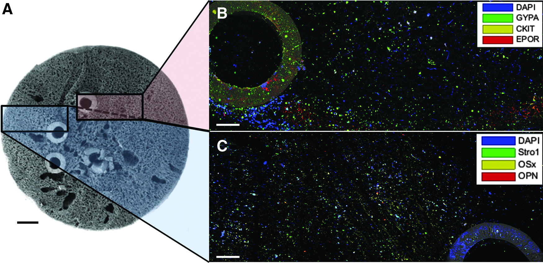
Imaging regions of the 3D culture device. (A) The topology of the hollow fiber bioreactor as a representative scanning electron micrograph cross-section and (B, C) surveyed five-color confocal images. Scale bar in (A) is 1 mm and in (B) and (C) is 100 μm, and bioreactor material reflection is represented in grayscale. Markers analyzed were 4′,6-diamidino-2-phenylindole for cell nuclei, and cell phenotypes: glycophorin-A (GYPA), erythropoietin receptor (EPO-R), and stem cell growth receptor (c-kit) shown in Figure 1B, and Stro-1 (Stro1), osterix (OSx), and osteopontin (OPN) shown in Figure 1C. 3D, three-dimensional. Color images available online at www.liebertpub.com/tec

IF sample preparation

For analyses, the 3D cultures were snap frozen in liquid nitrogen and preserved at −80°C until sectioning. Sectioning occurred at −20°C into thick histological sections of ∼1 mm. The frozen sections were directly fixed in ice cold 4% paraformaldehyde (BDH Laboratory Sciences, Poole, Dorset, United Kingdom) in phosphate-buffered saline (PBS; Life Technologies, Paisley, United Kingdom) overnight followed by a 2-h permeabilization with 0.1% Triton X-100 (Sigma-Aldrich, Poole, Dorset, United Kingdom) in staining buffer (1% bovine serum albumin [Sigma-Aldrich)], 0.5% Tween-20 [Promega, Southampton, Hampshire, United Kingdom], and 0.01% NaN3 [Sigma-Aldrich] in PBS). This was followed by a 4-h blocking step with 10% donkey serum (AbCam, Cambridge, United Kingdom) in staining buffer and overnight incubation with primary antibodies and isotype controls (Table 1; AbCam) in staining buffer at 4°C. Thereafter, 6-h staining was undertaken with secondary antibodies: donkey antirat Alexa Fluor 488, donkey antisheep Alexa Fluor 488 (AF488), donkey antirabbit Alexa Fluor 555 (AF555), and donkey antimouse Alexa Fluor 647 (AF647) all at 1:500 dilution in staining buffer at 4°C (Life Technologies). These steps were followed by a 4′,6-diamidino-2-phenylindole (DAPI) counterstain (Fisher Scientific, Loughborough, Leics, United Kingdom) overnight at 50 μM in PBS at 4°C, and samples were stored in 0.01% NaN₃ in PBS at 4°C. Each step was separated by single or multiple 15 min washing steps in appropriate buffer.

Table 1.

Confocal Three-Dimensional Immunofluorescent Microscopy Primary Antibody Staining Protocol

Figure 1B	Figure 1B isotype	Figure 1C	Figure 1C isotype	Unstained
1.7 μg/mL rat antihuman glycophorin-A (ab33386)	1.7 μg/mL rat IgG2b (ab18437)	6.7 μg/mL sheep antihuman Stro-1 (ab192766)	6.7 μg/mL sheep IgG (ab37385)	None
8.3 μg/mL rabbit antihuman C-Kit (ab111033)	8.3 μg/mL rabbit IgG (ab172730)	8.3 μg/mL rabbit antihuman osterix (ab94744)	8.3 μg/mL rabbit IgG (ab172730)	None
33.3 μg/mL mouse antihuman erythropoietin receptor (ab56310)	33.3 μg/mL mouse IgG2a (ab91361)	3.33 μg/mL mouse antihuman osteopontin (ab69498)	33.3 μg/mL mouse IgG2a (ab91361)	none

All products were obtained from AbCam with product number stated. The two samples presented in Figures 1 –5 were prepared alongside appropriate isotype and unstained controls.

IgG, immunoglobulin G.

Confocal microscopy image acquisition

The fixed, stained microscope sections were imaged on a Leica SP5 inverted confocal microscope with Leica LAS AF software (Leica, Milton Keynes, United Kingdom) using 405, 453, 488, 543, and 633 nm lasers and filters for DAPI, reflectance, AF488, AF555, and AF647 stains in two sequences of excitation for two-color collection then three-color collection without any detectable spill over. Images were taken at 512 × 512 pixel resolution using a 10 × dry microscope lens for a resolution of ∼3.03 μm per pixel with Z-stacks acquired in 5 μm slices, selected as the minimum lens magnification to ensure single-cell stain recognition.¹⁹ All laser voltage, filter wavelength, and capture settings were identical for corresponding samples and controls. Each sample was captured as three adjacent 3D images with 7% overlap to allow collation of three individual 1551 × 1551 μm² square images into a 4437 × 1551 μm² rectangular image with a depth of 350 μm for Figure 1B and 230 μm for Figure 1C. Unstained and isotype controls were captured under identical conditions. Images were not manipulated.

Cell localization

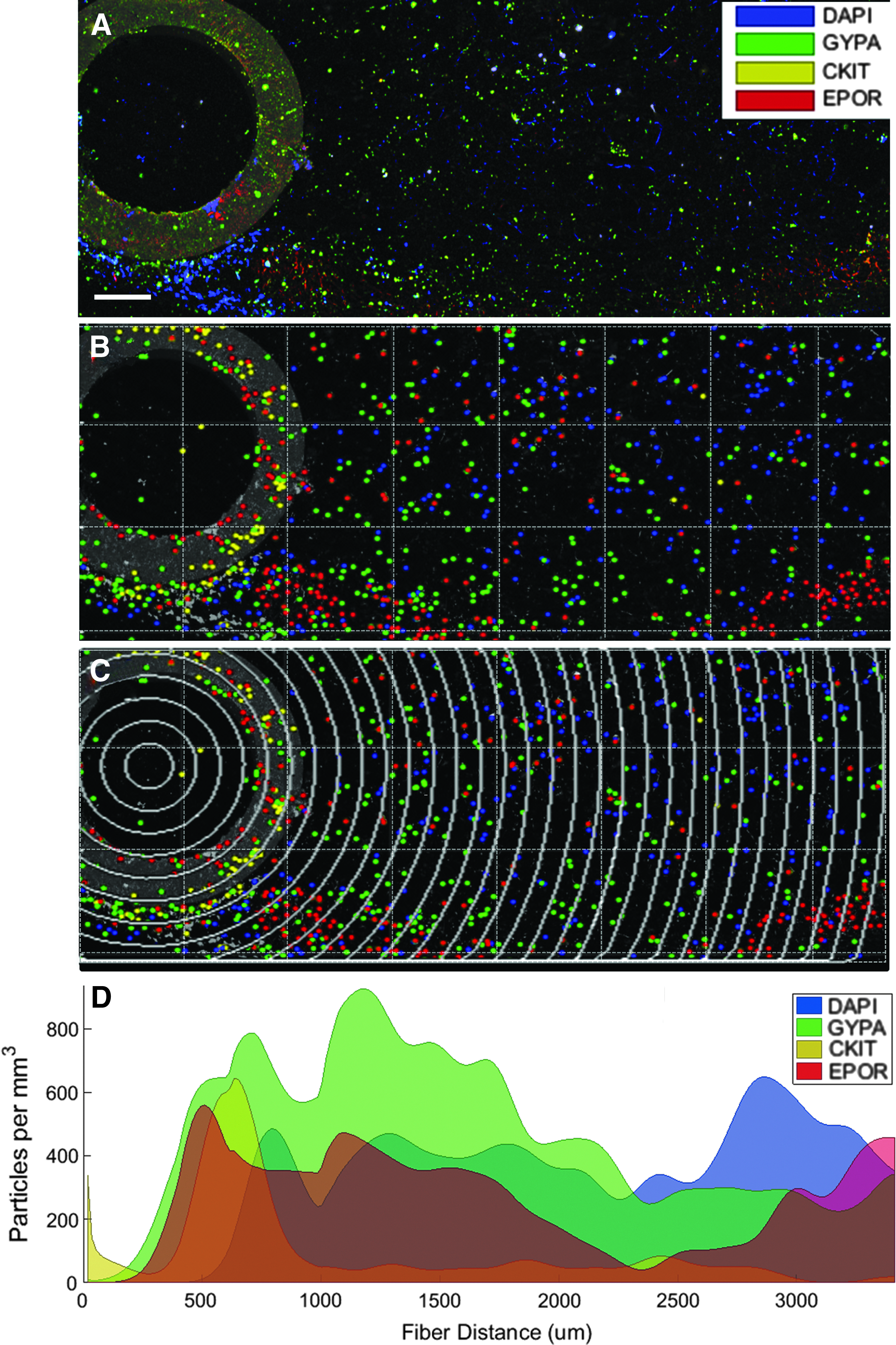
Once captured, images were analyzed using the Fiji image processing package of ImageJ: (1) the grid/collection package collated together adjacent 3D images, (2) the subtract background package decreased autofluorescence and self-absorbance, and, finally, (3) the 3D object counter package located the center of each individual fluorescence stain, (X,Y,Z)_c, which was exported into MATLAB for further analysis (The MathWorks, Inc., Natick, MA).^31–33 Representative confocal images are shown in Figure 1B and C in Table 2, with stain localization for Figure 1B shown in Figure 2A and B. The presence of each fluorescent antibody stain, (X,Y,Z)_c, was biologically validated in comparison with isotype controls, which contained <1% of detected sample stains. All computational postprocessing was run on a 3.4 GHz machine with 8 GB RAM and an Intel^® Core™ i7–4770 CPU. Processing times are provided and correspond as 1 s to 1.2 × 10⁸ random points sampled from a uniform distribution in MATLAB on this machine.

FIG. 2.

A visualization of the 2D distance cell density analysis. (A) Immunofluorescent images were captured and (B) fluorescent markers were identified by object-based colocalization. The fiber center was defined and (C) volumes of concentric spaces confined to image limits were calculated explicitly or estimated probabilistically to determine (D) cell and phenotype density at all distances captured by confocal microscopy. Scale bar in (A) is 100 μm. 2D, two-dimensional. Color images available online at www.liebertpub.com/tec

Table 2.

Mathematical Parameters

Parameter	Description	Ref.
(X,Y)_c; (X,Y,Z) _c	2D/3D cell position	^1,3
(X,Y)_a; (X,Y,Z)_a	Line or point of interest	^1,3
R_f	Cell-to-region of interest distance	^1,3
R_max	Maximum surveyable distance	—
A_i	Examined region area	²
R_i; R_i-1	Bin of examinable region	²
A_e; A_ee	Extraneous binned region area	²
V_L; (X,Y,Z)_L	Total image volume; limits	^4,5
V_i; V_i-1	Examined region volume	^4,5
V_LS; (X,Y,Z)_LS	Subset volume; limits	⁵

2D, two-dimensional; 3D, three-dimensional.

Two-dimensional distance distribution

Assessing cell density as a function of distance from an environmental region of interest is useful in examining cellular gradients across tissue sections.^14–19 To determine cellular distribution in 2D, 3D confocal image z-stacks (Fig. 1B) were compressed into 2D so that a given line of interest running perpendicular to the image plane becomes a point (X,Y)_a. Cellular heterogeneity was studied as a function of XY distance from this point of interest (Fig. 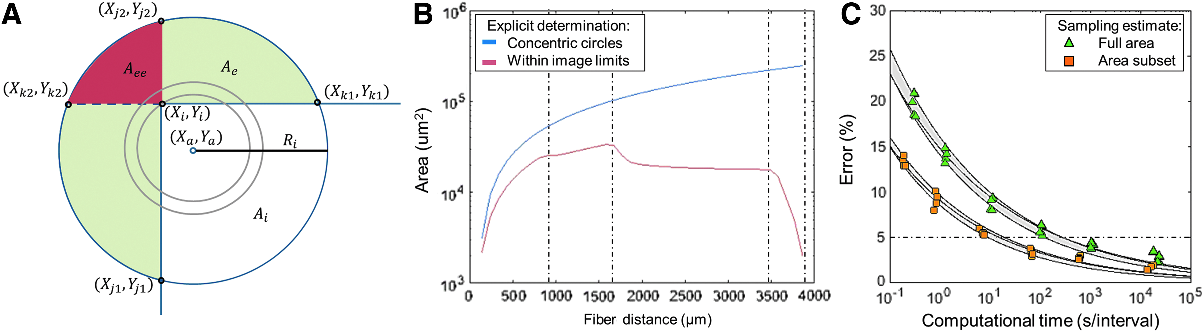2C, D), where individual cell position (X,Y)_c and its distance from the point of interest (X,Y)_a were defined as 2D Euclidean distance: \documentclass{aastex}\usepackage{amsbsy}\usepackage{amsfonts}\usepackage{amssymb}\usepackage{bm}\usepackage{mathrsfs}\usepackage{pifont}\usepackage{stmaryrd}\usepackage{textcomp}\usepackage{portland, xspace}\usepackage{amsmath, amsxtra}\usepackage{upgreek}\pagestyle{empty}\DeclareMathSizes{10}{9}{7}{6}\begin{document} \begin{align*} {R_c} = \sqrt {{{ \left( {{X_c} - {X_a}} \right) }^2} + {{ \left( {{Y_c} - {Y_a}} \right) }^2}} \tag{1} \end{align*} \end{document}

The full image field distance was defined as the distance from the point of interest to the furthest image pixel, R_max, and was then discretized into bins of radii, which form concentric circles of area \documentclass{aastex}\usepackage{amsbsy}\usepackage{amsfonts}\usepackage{amssymb}\usepackage{bm}\usepackage{mathrsfs}\usepackage{pifont}\usepackage{stmaryrd}\usepackage{textcomp}\usepackage{portland, xspace}\usepackage{amsmath, amsxtra}\usepackage{upgreek}\pagestyle{empty}\DeclareMathSizes{10}{9}{7}{6}\begin{document} $$\pi$$ \end{document} (R_i² − R_i-1²). Whenever the circle of radius R_i centered at (X,Y)_a encompassed space outside of the rectangular image limits, the extraneous area, A_e, was subtracted off for each breached side. In addition, if two of these breached sides overlapped to form a vertex of the rectangular limits, this overlapping extraneous area, A_ee, must be added back. The resulting equation becomes: \documentclass{aastex}\usepackage{amsbsy}\usepackage{amsfonts}\usepackage{amssymb}\usepackage{bm}\usepackage{mathrsfs}\usepackage{pifont}\usepackage{stmaryrd}\usepackage{textcomp}\usepackage{portland, xspace}\usepackage{amsmath, amsxtra}\usepackage{upgreek}\pagestyle{empty}\DeclareMathSizes{10}{9}{7}{6}\begin{document} \begin{align*} {A_i} = \pi \left( {R_i^2 - R_{i - 1}^2} \right) - {A_e} + {A_{ee}} \tag{2} \end{align*} \end{document}

Areas A_e and A_ee were arc angles of off-center circle area segments that were analytically calculated through a series of trigonometric identities (refer to Supplementary Data; Supplementary Data are available online at www.liebertpub.com/tec) and all terms correspond to Figure 3A and are summarized in Table 2. An illustration comparing concentric circle areas against concentric circle areas bounded to image limits (A_i) used in Figure 2 is shown in Figure 3B.

FIG. 3.

Two-dimensional tissue distance cell density analysis. (A) Mathematical notations used for 2D concentric neighborhoods surrounding the point of interest. (B) A visualization of concentric circle area (blue) and the area confined to discontinuous image limits (red) with iterative radii of 50 μm. (C) Monte Carlo estimation error from explicit solutions for successively tighter iterative Monte Carlo convergences (10⁻¹,…,10⁻⁶) averaged over four image geometries and 40 distance intervals per image inside (green) the full image cuboid or (orange) the smallest subset cuboid where trend lines were fitted to \documentclass{aastex}\usepackage{amsbsy}\usepackage{amsfonts}\usepackage{amssymb}\usepackage{bm}\usepackage{mathrsfs}\usepackage{pifont}\usepackage{stmaryrd}\usepackage{textcomp}\usepackage{portland, xspace}\usepackage{amsmath, amsxtra}\usepackage{upgreek}\pagestyle{empty}\DeclareMathSizes{10}{9}{7}{6}\begin{document} $$E = \;{k_1}{e^{ - {k_2} \ln t}}$$ \end{document} for the mean, m_E, and the 95% confidence interval, \documentclass{aastex}\usepackage{amsbsy}\usepackage{amsfonts}\usepackage{amssymb}\usepackage{bm}\usepackage{mathrsfs}\usepackage{pifont}\usepackage{stmaryrd}\usepackage{textcomp}\usepackage{portland, xspace}\usepackage{amsmath, amsxtra}\usepackage{upgreek}\pagestyle{empty}\DeclareMathSizes{10}{9}{7}{6}\begin{document} $$ { m_E } \pm 1.96 { \frac { { \sigma _E } } { \sqrt n } } $$ \end{document} for n = 4, shaded in gray. Color images available online at www.liebertpub.com/tec

To assess complex 3D geometries that can also be validated against analytical 2D solutions, Monte Carlo methods have been employed to estimate complex geometrical spaces by generating points from a uniform distribution within a measureable region, such as the complete image volume.³⁴ However, this method may be inaccurate when insufficient points are generated. Therefore, in the 2D case, estimation error was defined as the percentage difference of the Monte Carlo estimation from the analytical solution. As there was no analytical solution for many 3D cases, Monte Carlo convergence was defined as the percentage difference between estimated Monte Carlo solutions when 10⁴ additional uniformly generated points were appended.³⁵

The Monte Carlo method was validated for the typical 2D distance distribution (Fig. 3C) by calculating the average estimation error and Monte Carlo convergence across four image geometries, each broken into 40 equidistant intervals from a point of interest. An estimation error of 2.75% from the explicit calculation was reached for 10⁻⁶% Monte Carlo convergence in iterations of 10⁴ points, but required 8.6 min. A 10⁻²% Monte Carlo convergence, which corresponded to an average of 2.4 × 10⁶ generated points or 0.02 s per distance interval with estimation error less than 5% in the 2D distance distribution, was utilized for all subsequent distance distribution analyses.

3D distance distribution

The analysis of 3D cell distributions away from a specific point of interest is often utilized for cell colocalization studies, but is currently limited to cells either near the center of the image or only for very close cell proximities, creating regional bias in analysis.^{11–12,23,29} To analyze 3D cell distribution from a point of interest \documentclass{aastex}\usepackage{amsbsy}\usepackage{amsfonts}\usepackage{amssymb}\usepackage{bm}\usepackage{mathrsfs}\usepackage{pifont}\usepackage{stmaryrd}\usepackage{textcomp}\usepackage{portland, xspace}\usepackage{amsmath, amsxtra}\usepackage{upgreek}\pagestyle{empty}\DeclareMathSizes{10}{9}{7}{6}\begin{document} $${ \left( {X , Y , Z} \right) _a}$$ \end{document} throughout the entire image, the distance from \documentclass{aastex}\usepackage{amsbsy}\usepackage{amsfonts}\usepackage{amssymb}\usepackage{bm}\usepackage{mathrsfs}\usepackage{pifont}\usepackage{stmaryrd}\usepackage{textcomp}\usepackage{portland, xspace}\usepackage{amsmath, amsxtra}\usepackage{upgreek}\pagestyle{empty}\DeclareMathSizes{10}{9}{7}{6}\begin{document} $${ \left( {X , Y , Z} \right) _a}$$ \end{document} to the furthest pixel imaged was divided into intervals, R_i. Cell \documentclass{aastex}\usepackage{amsbsy}\usepackage{amsfonts}\usepackage{amssymb}\usepackage{bm}\usepackage{mathrsfs}\usepackage{pifont}\usepackage{stmaryrd}\usepackage{textcomp}\usepackage{portland, xspace}\usepackage{amsmath, amsxtra}\usepackage{upgreek}\pagestyle{empty}\DeclareMathSizes{10}{9}{7}{6}\begin{document} $${ \left( {X , Y , Z} \right) _c}$$ \end{document} exists within the interval \documentclass{aastex}\usepackage{amsbsy}\usepackage{amsfonts}\usepackage{amssymb}\usepackage{bm}\usepackage{mathrsfs}\usepackage{pifont}\usepackage{stmaryrd}\usepackage{textcomp}\usepackage{portland, xspace}\usepackage{amsmath, amsxtra}\usepackage{upgreek}\pagestyle{empty}\DeclareMathSizes{10}{9}{7}{6}\begin{document} $$\left( {{R_{i - 1}} , {R_i}} \right)$$ \end{document} if \documentclass{aastex}\usepackage{amsbsy}\usepackage{amsfonts}\usepackage{amssymb}\usepackage{bm}\usepackage{mathrsfs}\usepackage{pifont}\usepackage{stmaryrd}\usepackage{textcomp}\usepackage{portland, xspace}\usepackage{amsmath, amsxtra}\usepackage{upgreek}\pagestyle{empty}\DeclareMathSizes{10}{9}{7}{6}\begin{document} \begin{align*} {R_{i - 1}} < {R_c} = \sqrt {{{ \left( {{X_c} - {X_a}} \right) }^2} + {{ \left( {{Y_c} - {Y_a}} \right) }^2} + {{ \left( {{Z_c} - {Z_a}} \right) }^2}} \le {R_i}. \tag{3} \end{align*} \end{document}

Therefore, cell density within neighborhood \documentclass{aastex}\usepackage{amsbsy}\usepackage{amsfonts}\usepackage{amssymb}\usepackage{bm}\usepackage{mathrsfs}\usepackage{pifont}\usepackage{stmaryrd}\usepackage{textcomp}\usepackage{portland, xspace}\usepackage{amsmath, amsxtra}\usepackage{upgreek}\pagestyle{empty}\DeclareMathSizes{10}{9}{7}{6}\begin{document} $$\left( {{R_{i - 1}} , {R_i}} \right)$$ \end{document} can be calculated as the quantity of all cells within \documentclass{aastex}\usepackage{amsbsy}\usepackage{amsfonts}\usepackage{amssymb}\usepackage{bm}\usepackage{mathrsfs}\usepackage{pifont}\usepackage{stmaryrd}\usepackage{textcomp}\usepackage{portland, xspace}\usepackage{amsmath, amsxtra}\usepackage{upgreek}\pagestyle{empty}\DeclareMathSizes{10}{9}{7}{6}\begin{document} $$\left( {{R_{i - 1}} , {R_i}} \right)$$ \end{document} divided by the neighborhood's volume, V_i. If this neighborhood exists entirely within image boundaries, then the neighborhood volume is \documentclass{aastex}\usepackage{amsbsy}\usepackage{amsfonts}\usepackage{amssymb}\usepackage{bm}\usepackage{mathrsfs}\usepackage{pifont}\usepackage{stmaryrd}\usepackage{textcomp}\usepackage{portland, xspace}\usepackage{amsmath, amsxtra}\usepackage{upgreek}\pagestyle{empty}\DeclareMathSizes{10}{9}{7}{6}\begin{document} $$V_i = \frac { 4 } { 3 } \pi$$ \end{document} (R_i³−R_i-1³). However, if a portion of this neighborhood exists outside of the image boundaries, then calculation of V_i may not hold an explicit solution. In this case, Monte Carlo point sampling methods were implemented to estimate volume V_i: random 3D points \documentclass{aastex}\usepackage{amsbsy}\usepackage{amsfonts}\usepackage{amssymb}\usepackage{bm}\usepackage{mathrsfs}\usepackage{pifont}\usepackage{stmaryrd}\usepackage{textcomp}\usepackage{portland, xspace}\usepackage{amsmath, amsxtra}\usepackage{upgreek}\pagestyle{empty}\DeclareMathSizes{10}{9}{7}{6}\begin{document} $${P_N} = { \left( {X , Y , Z} \right) _N}$$ \end{document} were generated from a uniform distribution (known as Monte Carlo sampling) across the entire imaged space, such that \documentclass{aastex}\usepackage{amsbsy}\usepackage{amsfonts}\usepackage{amssymb}\usepackage{bm}\usepackage{mathrsfs}\usepackage{pifont}\usepackage{stmaryrd}\usepackage{textcomp}\usepackage{portland, xspace}\usepackage{amsmath, amsxtra}\usepackage{upgreek}\pagestyle{empty}\DeclareMathSizes{10}{9}{7}{6}\begin{document} $${P_N} \in \left[ { \left( {0 , 0 , 0} \right) , {{ \left( {X , Y , Z} \right) }_L}} \right]$$ \end{document} . Then, P_n is defined as the fraction of P_N within the sphere volume of interest, such that \documentclass{aastex}\usepackage{amsbsy}\usepackage{amsfonts}\usepackage{amssymb}\usepackage{bm}\usepackage{mathrsfs}\usepackage{pifont}\usepackage{stmaryrd}\usepackage{textcomp}\usepackage{portland, xspace}\usepackage{amsmath, amsxtra}\usepackage{upgreek}\pagestyle{empty}\DeclareMathSizes{10}{9}{7}{6}\begin{document} $${P_n} \in \left( {{{ \left( {X , Y , Z} \right) }_a} \pm {R_i}} \right)$$ \end{document} , and an estimate of concentric neighborhood volume is provided as \documentclass{aastex}\usepackage{amsbsy}\usepackage{amsfonts}\usepackage{amssymb}\usepackage{bm}\usepackage{mathrsfs}\usepackage{pifont}\usepackage{stmaryrd}\usepackage{textcomp}\usepackage{portland, xspace}\usepackage{amsmath, amsxtra}\usepackage{upgreek}\pagestyle{empty}\DeclareMathSizes{10}{9}{7}{6}\begin{document} \begin{align*} { V_i } = { V_L } { \frac { \sum { P_n } } { \sum { P_N } } } - { V_ { i - 1 } } , \tag { 4 } \end{align*} \end{document}

where V_L is the full image volume and the concentric neighborhood volume of the prior radial interval R_i−1 is given by V_i−1. This process of uniform point generation and volume calculation was repeated and appended until iterations of calculated V_i vary less than a chosen Monte Carlo convergence limit, as already discussed. The estimation of a 100 μm cell neighborhood (100 μm, 4.2 × 10⁻³ mm³) inside a large image volume, V_L (2.4 mm³), required sampling 5.8 × 10⁷ uniformly distributed random points and 0.49 s, or 9.1 min if repeated for the 1116 cells within Figure 1B.

FIG. 4.

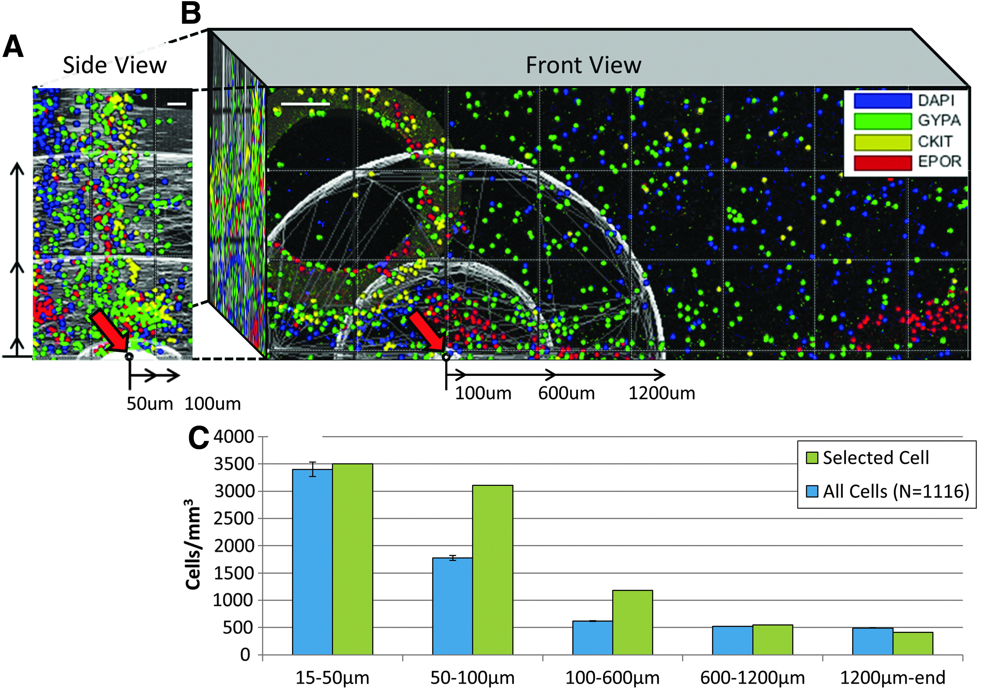
A visualization of the 3D cell clustering density analysis in confocal images. (A, B) A cell of interest was defined and volumes of concentric spheres confined to image limits were estimated through point sampling to determine (C) cell density at any imaged neighborhoods away from a given cell (red arrow, green bars), which can then be iterated for all 1116 (±SEM) cells throughout the image (blue bars). Scale bars in (A, B) are 100 μm. SEM, standard error of the mean. Color images available online at www.liebertpub.com/tec

Computational time decreased by 96% from 9.1 min to 22 s when Monte Carlo point sampling methods were applied within small regions around each cell rather than across the entire image space. A smaller cuboid of known volume, V_LS, was constructed to exactly encase the cell neighborhood [volume (2R_i)³ centered on cell \documentclass{aastex}\usepackage{amsbsy}\usepackage{amsfonts}\usepackage{amssymb}\usepackage{bm}\usepackage{mathrsfs}\usepackage{pifont}\usepackage{stmaryrd}\usepackage{textcomp}\usepackage{portland, xspace}\usepackage{amsmath, amsxtra}\usepackage{upgreek}\pagestyle{empty}\DeclareMathSizes{10}{9}{7}{6}\begin{document} $${ \left( {X , Y , Z} \right) _c}$$ \end{document} ] that was then confined within the image limits (V_LS ≤ 8 × 10⁻³ mm³ for R_i = 100 μm cell neighborhood). Points, \documentclass{aastex}\usepackage{amsbsy}\usepackage{amsfonts}\usepackage{amssymb}\usepackage{bm}\usepackage{mathrsfs}\usepackage{pifont}\usepackage{stmaryrd}\usepackage{textcomp}\usepackage{portland, xspace}\usepackage{amsmath, amsxtra}\usepackage{upgreek}\pagestyle{empty}\DeclareMathSizes{10}{9}{7}{6}\begin{document} $${P_{NS}}$$ \end{document} , were sampled within the cuboid subvolume such that \documentclass{aastex}\usepackage{amsbsy}\usepackage{amsfonts}\usepackage{amssymb}\usepackage{bm}\usepackage{mathrsfs}\usepackage{pifont}\usepackage{stmaryrd}\usepackage{textcomp}\usepackage{portland, xspace}\usepackage{amsmath, amsxtra}\usepackage{upgreek}\pagestyle{empty}\DeclareMathSizes{10}{9}{7}{6}\begin{document} $${P_{NS}} \in {V_{LS}} \subset {V_L}$$ \end{document} , and the fraction of \documentclass{aastex}\usepackage{amsbsy}\usepackage{amsfonts}\usepackage{amssymb}\usepackage{bm}\usepackage{mathrsfs}\usepackage{pifont}\usepackage{stmaryrd}\usepackage{textcomp}\usepackage{portland, xspace}\usepackage{amsmath, amsxtra}\usepackage{upgreek}\pagestyle{empty}\DeclareMathSizes{10}{9}{7}{6}\begin{document} $${P_{NS}}$$ \end{document} within the sphere volume of interest, \documentclass{aastex}\usepackage{amsbsy}\usepackage{amsfonts}\usepackage{amssymb}\usepackage{bm}\usepackage{mathrsfs}\usepackage{pifont}\usepackage{stmaryrd}\usepackage{textcomp}\usepackage{portland, xspace}\usepackage{amsmath, amsxtra}\usepackage{upgreek}\pagestyle{empty}\DeclareMathSizes{10}{9}{7}{6}\begin{document} $${P_{nS}} \in \left( {{{ \left( {X , Y , Z} \right) }_a} \pm {R_i}} \right)$$ \end{document} , provided a more efficient estimate of concentric neighborhood volume than sampling points within the entire image limits as \documentclass{aastex}\usepackage{amsbsy}\usepackage{amsfonts}\usepackage{amssymb}\usepackage{bm}\usepackage{mathrsfs}\usepackage{pifont}\usepackage{stmaryrd}\usepackage{textcomp}\usepackage{portland, xspace}\usepackage{amsmath, amsxtra}\usepackage{upgreek}\pagestyle{empty}\DeclareMathSizes{10}{9}{7}{6}\begin{document} \begin{align*} { V_i } = { V_ { LS } } { \frac { \sum { P_ { nS } } } { \sum { P_ { NS } } } } - { V_ { i - 1 } } . \tag { 5 } \end{align*} \end{document}

Fewer sampled points were required within V_LS than V_L to reach the same Monte Carlo convergence: 2.4 × 10⁶ uniformly distributed random points required 0.02 s per cell neighborhood, or 22 s for all 1116 cells shown in Figure 1B. Using the proposed method, 3D cell density distributions can be quickly analyzed at distances up to half the diagonal image distance, or \documentclass{aastex}\usepackage{amsbsy}\usepackage{amsfonts}\usepackage{amssymb}\usepackage{bm}\usepackage{mathrsfs}\usepackage{pifont}\usepackage{stmaryrd}\usepackage{textcomp}\usepackage{portland, xspace}\usepackage{amsmath, amsxtra}\usepackage{upgreek}\pagestyle{empty}\DeclareMathSizes{10}{9}{7}{6}\begin{document} $$0.5 \sqrt {X_L^2 + Y_L^2 + Z_L^2}$$ \end{document} , for every cell present in the image.

Alternatively, an equally spaced 3D grid of k points across the image volume, V_L, or a similar image subvolume, V_LS, can be used to estimate cell neighborhoods. However, iterative grid generations must be performed with \documentclass{aastex}\usepackage{amsbsy}\usepackage{amsfonts}\usepackage{amssymb}\usepackage{bm}\usepackage{mathrsfs}\usepackage{pifont}\usepackage{stmaryrd}\usepackage{textcomp}\usepackage{portland, xspace}\usepackage{amsmath, amsxtra}\usepackage{upgreek}\pagestyle{empty}\DeclareMathSizes{10}{9}{7}{6}\begin{document} $${ \left( {2k} \right) ^3}$$ \end{document} additional points, which greatly increases computational time, and is discussed as a different method to random point generation from a uniform distribution (refer to Supplementary Data, Supplementary Fig. S2).

Statistics

Quantitative results are represented as mean ± standard error of four replicate experimental samples prepared and assessed identically (Fig. 1B), or four replicate computationally generated samples as stated.

Results

Enhanced utilization of imaged data

The presented algorithms completely assess 2D and 3D cell density distributions of imaged histological data, whereas current methods disregard data near image boundaries.^11–13 Therefore, the algorithms herein enhance utilization of image data in two ways: (i) by surveying more points of interest and (ii) by probing further distances from each point of interest. With current approaches, an ideally centered point of interest within Figure 1B could only be inspected up to a maximum 2D distance of 775 μm (the closest image boundary); in contrast, using the presented algorithms, a 2D distribution of at minimum 2300 μm (the furthest imaged pixel) can now be calculated from any point within the image.

Cell density distribution algorithms are typically repeated for multiple points, or cells, of interest. A conservative comparison with current methods was performed by analyzing 3D cell density distributions within a 100 μm neighborhood around every cell to demonstrate cell-to-cell association as shown in Figure 1B (similar to Bjornsson et al.¹¹). Current methods utilize only cells further than 100 μm from an image boundary as points of interest (N = 524), whereas with the presented approach, all imaged cells were utilized (N = 1116) at a 23-fold greater distance. The inclusion of these cells improved cell density estimations by 26% and 23% within 15–50 and 50–100 μm intervals, respectively.

Accurate manual scoring allows for the exact measurement of cell positions and cell-to-cell distances, but would be infeasible to manually pinpoint thousands of cells in a large image and infeasible to measure the hundreds of thousands of intracellular distances and the volumetric neighborhoods to calculate cellular density distributions within. The proposed algorithm was compared to manual scoring of random fractions of the entire image shown in Figure 1B, which revealed that partial manual scoring reduced accuracy because of the nonuniform distribution of cells and was unable to analyze cell distributions at long distances as described in the Supplementary Data, while still reducing analysis time from 30 min down to 1 min.

Random sampling accuracy

The point sampling algorithm was validated by assessing uniformly generated random cell distributions, as shown in Figure 5A. These data sets comprised four types of 500 computationally generated cells, which were uniformly distributed within a 4437 × 1551 × 230 μm³ space to produce a known cell density while replicating the number of cells and image geometry of experimental samples, as performed in current studies.^14,15 The sampling method accurately analyzed the uniform distribution of cells, where 2000 uniformly generated cell positions were found to have an average of 1257.6 ± 44.8, 1244.8 ± 22.4, and 1297.2 ± 2.0 cells/mm³ in 15–50, 50–100, and 100–600 μm neighborhoods of all other cells, and 1297.0 ± 0.2 cells/mm³ throughout the remaining 2300 μm of the image space (n = 2000 cells). Small 50 and 100 μm neighborhoods contained significantly smaller number of cells, and may have accounted for their higher variability, but even so the density of cells was found to closely approximate a uniform distribution of 2000 cells in the image volume of 1.54 mm³.

FIG. 5.

Assessment of methods and applications for calculating 3D cell clustering density. (A) Cell clustering density estimation for four iterations (±SEM, red) of four types of 500 computationally generated cells, or, for (B) cells imaged from a hollow fiber bioreactor with and (C) without the hollow fiber region, representing a spatial asymmetry. Scale bars in (A–C) are 100 μm. Objects analyzed (D–F) include randomized control cells (RC1–RC4), as well as fluorescent markers. Color images available online at www.liebertpub.com/tec

Three-dimensional distribution with regional asymmetries

Many histological images contain gaps or spaces without cells, such as vessels, areas of decalcified bone, or the edge of the sectioned sample. These voids may underestimate cell density during computational analysis if they are averaged into dense cellular neighborhoods. However, if a significantly larger number of cells could be assessed with full image field analysis, regional asymmetries might be more accurately determined. Cell clustering density analyses were run on an identical image, including or excluding regions with engineered void space (Fig. 5B, C), and showed that the region containing the voidage played a relatively minor role in influencing paracrine cell–cell niche communication, but a much greater regional effect correlating with its inclusion or exclusion from the 2D distance cell density analysis. There was a 7.8%, 11.1%, and 44.6% difference in cell density in 15–50, 50–100, and 100–600 μm neighborhoods between the image with and without the fiber, and a 46.2% difference in cell density throughout the rest of the image, demonstrating that this regional phenomenon altered cell localization at large 2D tissue scales, but cell association at close intercellular distances remained consistent throughout the image.

Discussion

Three-dimensional image analyses enable the acquisition of information on spatial cell and tissue heterogeneity because of their quantitative algorithms.^6,7 However, current calculations of cell distributions are often constrained to a central subset of the image provided, and are further limited when phenomena of interest are off-center or replicate events per image are assessed. When the entire tissue volume of interest is infeasible to image, recent studies have compensated by quantitating images of incomplete tissue subsections either through normalization against uniformly generated random data within a similar tissue topology^13–15 or by only analyzing phenomena that exist within the most central subsection of the image.^11–12,16 The former method only provides relative quantitation of images, whereas the later discards nearly half of 3D imaged data.^11,12 The presented analyses in this study quantitate 2D and 3D distributions of phenomena throughout any full image, providing a minimum 50-fold increase in analytical range (increased distance times increased cells analyzed) throughout coupling complex Euclidean metrics with Monte Carlo point sampling estimations.

The analysis of cell distributions can be parametrically tuned for computational speed and analytical resolution to avoid miscalculation. Analytical resolution is dependent on the number of regions the image is partitioned into and, for 3D distributions, the Monte Carlo simulation is also dependent on the quantity of uniformly generated random points. The partitioning of image regions is a balance of precision, where larger, coarser partitions may average local spatial phenomena into a larger population of cells, whereas smaller, finer partitions could provide misleading cell densities because of the sharp geometrical discontinuities that exist at image boundaries and the small number of cells that exist within small partitions. The partition balance is observed as the measurement of small cell proximal 3D regions held larger error (4% standard error at 0.0042 mm³) than larger, cell distal 3D regions (0.015% standard error at 2.4 mm³). The generation of sufficient quantities of uniformly generated random points to estimate complex 3D volumes is dependent on system and user-specific error tolerance; in the presented case, an average of 2.4 × 10⁶ points were generated, which yielded a 5% error when compared against known controls, as already discussed.

Many studies of cell recognition and cell–cell or cell–tissue colocalization have avoided the need for efficient image analysis algorithms by capturing multiple or larger images at lower magnification, increasing the cost and time of these already demanding techniques. Morales-Navarrete et al.³⁶ proposed imaging at a moderate resolution (25 × , 1 μm³ voxel), then retiling parts of this low-resolution image with high resolution (63 × , 0.03 μm³ voxel) to capture both vasculature of ∼100–300 μm diameters for murine liver reconstruction followed by cellular and subcellular reconstruction of hepatocytes. Studies by Khorshed et al.¹⁹ and Sundaramurthy et al.³⁷ enumerated intravital murine hematopoietic cells at moderate resolutions (20–40 × , 0.2–7.3 μm³ voxel) to inspect intracellular and intercellular activity for small populations of ∼25 cells. The presented study depicts cells at significantly lower resolution (10 × , 46 μm³ voxel), as an optimal balance between image volume analyzed at a tissue scale while still capturing many hematopoietic cells (1000's of 500–33,500 μm³ cells) at high enough resolution to pinpoint cell nuclei and associated fluorescent markers among their environment. This lower magnification and resolution has also been employed in semiautomatic cell and fluorescent marker identification in 3D tissue cultures³⁸ to assess megakaryocyte distance from vascularization in murine bone marrow,³⁹ and used as standard images to compare cell motion tracking algorithms across 14 laboratories.⁴⁰

The quantitative evaluation of cellular density and heterogeneity is frequently studied and used in vitro and in vivo 3D applications inspecting roles of cellular and environmental interactions. Many 3D culture systems employ surfaces, scaffolds, carriers, or fibers as an aim to impart spatial heterogeneity to mimic and, upon implantation, integrate with many tissue asymmetries present physiologically.^{1–4,25–28} Pinpointing cell niche placement and cell association as a tool toward developmental understanding, tracking disease progression, and mammalian cell culture bioprocess design has become increasingly studied in ex vivo analogues; however, few intravital analyses have been performed until recently, and none in the adult human.^{14–29,36–40} Cell colocalization algorithms frequently inspect small distances from cells or tissues of interest such as the effect of high oxygen tension on cells within 150 μm of a vascular sinus and the migration of cells within 100 μm of bone surfaces.^16,19 The assessment of spatial heterogeneity away from more complex regions of interest, such as uneven bone surfaces or noncircular vessel walls, could utilize these proposed algorithms to capture the full image field in one of two ways: in an identical method if these phenomena can be described as a function, or through an iterative process once the complex phenomena of interest have been meshed or mapped similar to the detection of the murine marrow bone surface by Khorshed et al.¹⁹

These algorithms are capable of being applied to any quantitative 3D imaging platform, including magnetic resonance imaging (MRI), computed tomography (CT), and optical imaging (UV, visible, IR) because of their use of spatially “tagged” contrast agents or probes (e.g., nanomaterials, labeled small and large molecules, and fluorescent proteins), where discrete cells, phenomena, or regions of interest can be spatially identified.^6,7 MRI and CT imaging allow for full specimen penetration but lack multiplexed probe detection, have poorer sensitivity, and lower resolution; only recent advancements have allowed imaging at single-cell resolution.⁶ Optical imaging allows for the quantitative analysis of a wide variety of cell–environment interactions and can characterize multiple phenotypes, organelle, and matrix proteins simultaneously by implementing light microscopy with immunohistochemistry or IF imaging of probes and chemicals delineating cell or tissue type, status, and their interactions to quantify the effects of the tissue environment on cell differentiation, proliferation, and stimulation spatially at multiple aspect sizes.^8,9 The versatility of optical imaging is frequently implemented to determine quantitative colocalization from the subcellular protein-scale up to multicellular and tissue scales.^10–28

The complete quantitative utilization of 3D imaged space is required to leverage the high cost of native or engineered tissue histology. The study of spatial heterogeneity in tissue constructs has become increasingly popular from both advancements in 3D culture systems to mimic physiological structures and functions and advancements in imaging technologies able to better define the performance of natural and engineered cellular environments. The presented image analyses, for the first time, pair Euclidean metrics with Monte Carlo estimations to determine colocalization across the entire imaged data set, assessing 2.2-fold more area per frame in 2D distance metrics to depict cell populations in more distant, peripheral imaged areas from phenomena of interest. In 3D distance metrics, all cell neighborhoods can be analyzed to half the maximum image length, whereas basic algorithms may only assess one perfectly central cell per image; hence, these tools provide 10²–10⁴ more replicate cell measurements per image at a similar, if not greater, scope. The fabrication, culture, and analysis of tissue -engineered and clinical samples for image analysis represent a time-, labor-, and cost-intensive process, and efficient post-analysis tools to quantitatively assess the full image field, as presented here, are needed to detail cellular interactions among their environment.

Footnotes

Acknowledgments

This work is supported by ERC-BioBlood (No. 340719), the Richard Thomas Leukaemia Research Fund, and a Royal Academy of Engineering Fellowship to R.M. M.C.A. is grateful for the Imperial College Chemical Engineering Scholarship. The authors are grateful to Deborah Keller and Stephen Rothery of Imperial College's Core FILM Facilities for the useful discussions.

Disclosure Statement

No competing financial interests exist.

References

Cha

, Liechty

W.B.

, Khademhosseini

, and Peppas

N.A.

Designing biomaterials to direct stem cell fate. ACS Nano, 6, 9353, 2012.

Pampaloni

, Reynaud

E.G.

, and Stelzer

E.H.K.

The third dimension bridges the gap between cell culture and live tissue. Nat Rev Mol Cell Biol, 8, 839, 2007.

Baker

B.M.

, and Chen

C.S.

Deconstructing the third dimension: how 3D culture microenvironments alter cellular cues. J Cell Sci, 125, 3015, 2012.

Khademhosseini

, Langer

, Borenstein

, and Vacanti

J.P.

Microscale technologies for tissue engineering and biology. Proc Natl Acad Sci U S A, 103, 2480, 2006.

Niklason

L.E.

, Yeh

A.T.

, Calle

E.A.

, Bai

, Valentín

, and Humphrey

J.D.

Enabling tools for engineering collagenous tissues integrating bioreactors, intravital imaging, and biomechanical modeling. Proc Natl Acad Sci U S A, 107, 3335, 2010.

Appel

A.A.

, Anastasio

M.A.

, Larson

J.C.

, and Brey

E.M.

Imaging challenges in biomaterials and tissue engineering. Biomaterials, 34, 6615, 2013.

Weissleder

, and Nahrendorf

Advancing biomedical imaging. Proc Natl Acad Sci U S A, 112, 14424, 2015.

Ntziachristos

Going deeper than microscopy: the optical imaging frontier in biology. Nat Methods, 7, 603, 2010.

Flower

M.A.

(ed.). Webb's Physics of Medical Imaging. Boca Raton, FL: CRC Press, 2012.

10.

Ntziachristos

Floresence molecular imaging. Annu Rev Biomed Eng, 8, 1, 2006.

11.

Bjornsson

C.S.

, Lin

, Al-Kofahi

, Narayanaswamy

, Smith

K.L.

, Shain

, and Roysam

Associative image analysis: a method for automated quantification of 3D multi-parameter images of brain tissue. J Neurosci Methods, 170, 165, 2008.

12.

Delarue

, Joanny

J.F.

, Jülicher

, and Prost

Stress distributions and cell flows in a growing cell aggregate. Interface Focus, 4, 20140033, 2014.

13.

Meddens

M.B.

, Rieger

, Figdor

C.G.

, Cambi

, and Van Den Dries

Automated podosome identification and characterization in fluorescence microscopy images. Microsc Microanal, 19, 180, 2013.

14.

Acar

, Kocherlakota

K.S.

, Murphy

M.M.

, Peyer

J.G.

, Oguro

, Inra

C.N.

, Jaiyeola

, Zhao

, Luby-Phelps

, and Morrison

S.J.

Deep imaging of bone marrow shows non-dividing stem cells are mainly perisinusoidal. Nature, 526, 126, 2015.

15.

Takaku

, Malide

, Chen

, Calado

R.T.

, Kajigaya

, and Young

N.S.

Hematopoiesis in 3 dimensions: human and murine bone marrow architecture visualized by confocal microscopy. Blood, 116, e41, 2010.

16.

Nombela-Arrieta

, Pivarnik

, Winkel

, Canty

K.J.

, Harley

, Mahoney

J.E.

, Park

S.Y.

, Lu

, Protopopov

, and Silberstein

L.E.

Quantitative imaging of haematopoietic stem and progenitor cell localization and hypoxic status in the bone marrow microenvironment. Nat Cell Biol, 15, 533, 2013.

17.

Celso

C.L.

, Fleming

H.E.

, Wu

J.W.

, Zhao

C.X.

, Miake-Lye

, Fujisaki

, Côté

, Rowe

D.W.

, Lin

C.P.

, and Scadden

D.T.

Live-animal tracking of individual haematopoietic stem/progenitor cells in their niche. Nature, 457, 92, 2009.

18.

Spencer

J.A.

, Ferraro

, Roussakis

, Klein

, Wu

, Runnels

J.M.

, Zaher

, Mortensen

L.J.

, Alt

, Turcotte

, and Yusuf

Direct measurement of local oxygen concentration in the bone marrow of live animals. Nature, 508, 269, 2014.

19.

Khorshed

R.A.

, Hawkins

E.D.

, Duarte

, Scott

M.K.

, Akinduro

O.A.

, Rashidi

N.M.

, Spitaler

, and Celso

C.L.

Automated identification and localization of hematopoietic stem cells in 3D intravital microscopy data. Stem Cell Rep, 5, 139, 2015.

20.

Bertrand

J.Y.

, Kim

A.D.

, Violette

E.P.

, Stachura

D.L.

, Cisson

J.L.

, and Traver

Definitive hematopoiesis initiates through a committed erythromyeloid progenitor in the zebrafish embryo. Development, 134, 4147, 2007.

21.

Vera

, and Zon

L.I.

High throughput in vivo phenotyping: the zebrafish as a tool for drug discovery for hematopoietic stem cells and cancer. Drug Discov Today Dis Models, 10, e17, 2013.

22.

Thon

J.N.

, Mazutis

, Wu

, Sylman

J.L.

, Ehrlicher

, Machlus

K.R.

, Feng

, Lu

, Lanza

, Neeves

K.B.

, and Weitz

D.A.

Platelet bioreactor-on-a-chip. Blood, 124, 1857, 2014.

23.

, Wang

, Loskill

, Huebsch

, Koo

, Svedlund

F.L.

, Marks

N.C.

, Hua

E.W.

, Grigoropoulos

C.P.

, Conklin

B.R.

, and Healy

K.E.

Self-organizing human cardiac microchambers mediated by geometric confinement. Nat Commun, 6, 7413, 2015.

24.

Toh

Y.C.

, Xing

, and Yu

Modulation of integrin and E-cadherin-mediated adhesions to spatially control heterogeneity in human pluripotent stem cell differentiation. Biomaterials, 50, 87, 2015.

25.

Di Buduo

C.A.

, Wray

L.S.

, Tozzi

, Malara

, Chen

, Ghezzi

C.E.

, Smoot

, Sfara

, Antonelli

, Spedden

, and Bruni

Programmable 3D silk bone marrow niche for platelet generation ex vivo and modeling of megakaryopoiesis pathologies. Blood, 125, 2254, 2015.

26.

Frezza

, Wouters

B.G.

, and McGuigan

A.P.

A three-dimensional engineered tumour for spatial snapshot analysis of cell metabolism and phenotype in hypoxic gradients. Nat Mater, 15, 227, 2016.

27.

Eng

, Lee

B.W.

, Parsa

, Chin

C.D.

, Schneider

, Linkov

, Sia

S.K.

, and Vunjak-Novakovic

Assembly of complex cell microenvironments using geometrically docked hydrogel shapes. Proc Natl Acad Sci U S A, 110, 4551, 2013.

28.

Rnjak‐Kovacina

, Wray

L.S.

, Golinski

J.M.

, and Kaplan

D.L.

Arrayed hollow channels in silk‐based scaffolds provide functional outcomes for engineering critically sized tissue constructs. Adv Funct Mater, 24, 2188, 2014.

29.

Liu

, Gerner

M.Y.

, Van Panhuys

, Levine

A.G.

, Rudensky

A.Y.

, and Germain

R.N.

Immune homeostasis enforced by co-localized effector and regulatory T cells. Nature, 528, 225, 2015.

30.

Panoskaltsis

, Macedo

H.M.M.

, Blanco

M.T.M.

, Mantalaris

, and Livingston

A.G.

3D Hollow Fibre Bioreactor Systems for the Maintenance, Expansion, Differentiation, and HARVEsting of Human Stem Cells and their Progeny Patent. WO 2012/069841 A1, 2012.

31.

Schindelin

, Arganda-Carreras

, Frise

, Kaynig

, Longair

, Pietzsch

, Preibisch

, Rueden

, Saalfeld

, Schmid

, and Tinevez

J.Y.

Fiji: an open-source platform for biological-image analysis. Nat Methods, 9, 676, 2012.

32.

Preibisch

, Saalfeld

, and Tomancak

Globally optimal stitching of tiled 3D microscopic image acquisitions. Bioinformatics, 25, 1463, 2009.

33.

Bolte

, and Cordelieres

F.P.

A guided tour into subcellular colocalization analysis in light microscopy. J Microsc, 224, 213, 2006.

34.

Smith

R.L.

Efficient Monte Carlo procedures for generating points uniformly distributed over bounded regions. Oper Res, 32, 1296, 1984.

35.

Cowles

M.K.

, and Carlin

B.P.

Markov chain Monte Carlo convergence diagnostics: a comparative review. Am Stat Assoc, 91, 883, 1994.

36.

Morales-Navarrete

, Segovia-Miranda

, Klukowski

, Meyer

, Nonaka

, Marsico

, Chernykh

, Kalaidzidis

, Zerial

, and Kalaidzidis

A versatile pipeline for the multi-scale digital reconstruction and quantitative analysis of 3D tissue architecture. eLife, 4, e11214, 2015.

37.

Sundaramurthy

, Barsacchi

, Chernykh

, Stöter

, Tomschke

, Bickle

, Kalaidzidis

, and Zerial

Deducing the mechanism of action of compounds identified in phenotypic screens by integrating their multiparametric profiles with a reference genetic screen. Nat Protoc, 9, 474, 2014.

38.

De Boodt

, Poursaberi

, Schrooten

, Berckmans

, and Aerts

J.M.

A semiautomatic cell counting tool for quantitative imaging of tissue engineering scaffolds. Tissue Eng Part C Methods, 19, 697, 2013.

39.

Malara

, Currao

, Gruppi

, Celesti

, Viarengo

, Buracchi

, Laghi

, Kaplan

D.L.

, and Balduini

Megakaryocytes contribute to the bone marrow‐matrix environment by expressing fibronectin, type IV collagen, and laminin. Stem Cells, 32, 926, 2014.

40.

Chenouard

, Smal

, De Chaumont

, Maška

, Sbalzarini

I.F.

, Gong

, Cardinale

, Carthel

, Coraluppi

, Winter

, and Cohen

A.R.

Objective comparison of particle tracking methods. Nat Methods, 11, 281, 2014.

Supplementary Material

Please find the following supplemental material available below.

For Open Access articles published under a Creative Commons License, all supplemental material carries the same license as the article it is associated with.

For non-Open Access articles published, all supplemental material carries a non-exclusive license, and permission requests for re-use of supplemental material or any part of supplemental material shall be sent directly to the copyright owner as specified in the copyright notice associated with the article.

0.50 MB

0.00 MB