A New Automated Histomorphometric MATLAB Algorithm for Immunohistochemistry Analysis Using Whole Slide Imaging

Abstract

The use of animal models along with the employment of advanced and sophisticated stereological methods for assessing bone quality combined with the use of statistical methods to evaluate the effectiveness of bone therapies has made it possible to investigate the pathways that regulate bone responses to medical devices. Image analysis of histomorphometric measurements remains a time-consuming task, as the image analysis software currently available does not allow for automated image segmentation. Such a feature is usually obtained by machine learning and with software platforms that provide image-processing tools such as MATLAB. In this study, we introduce a new MATLAB algorithm to quantify immunohistochemically stained critical-sized bone defect samples and compare the results with the commonly available Aperio Image Scope Positive Pixel Count (PPC) algorithm. Bland and Altman analysis and Pearson correlation showed that the measurements acquired with the new MATLAB algorithm were in excellent agreement with the measurements obtained with the Aperio PPC algorithm, and no significant differences were found within the histomorphometric measurements. The ability to segment whole slide images, as well as defining the size and the number of regions of interest to be quantified, makes this MATLAB algorithm a potential histomorphometric tool for obtaining more objective, precise, and reproducible quantitative assessments of entire critical-sized bone defect image data sets in an efficient and manageable workflow.

Impact statement

The introduced MATLAB algorithm provides a new, objective, histomorphometric image analysis process for use with immunohistochemically stained tissue samples. Unlike traditional manual methods, the algorithm is configured for efficient use requiring relatively minimal expertise, decreasing the required amount of time for processing while achieving high-quality quantitative analysis. The algorithm is demonstrated here for the analysis of stained bone and soft tissue histological sections, especially those typical of large animal studies; however, it can be applied to any immunohistochemically stained tissue sections.

Introduction

Although most bone defects heal spontaneously, under pathological conditions bone loss may happen in critical quantities in which bone will not heal without clinical intervention.¹ Despite increased controversy about what is defined as a critical-sized bone defect, a specific length has not been agreed on. However, a defect length >1–2 cm, as well as bone loss considered >50% of the defect circumference have been suggested as parameters for critical-sized bone defects.²

Extensive investigations have been carried out using tissue engineered constructs (TECs) in combination with autologous bone grafts, vascularized cortical periosteal flaps, mesenchymal stem cells (MSCs), platelet-rich plasma (PRP), and bone growth factors (BMPs) as potential alternative techniques to the current clinical bone graft materials used in the reconstruction of critical-sized bone defects.^3–13 However, how the application of these TECs coordinate the temporal and spatial interactions between cells and the TEC in terms of mimicking the natural structure of the extracellular matrix (ECM) of native bone tissue remains to be fully elucidated.

Most articles related to bone research are often scientifically reasoned by X-rays, mechanical testing, microcomputed tomography evaluation, histological and immunohistochemical assessment, scanning electron microscopy (SEM), quantitative backscattered electron imaging (BSE), confocal laser scanning microscopy, as well as energy dispersive X-ray microanalysis (EDX) and synchrotron small angle X-ray scattering (SAXS).^{4,6,7,9–11,13–18} Owing to the hierarchical structure of these bone TECs, cell-to-cell and cell-to-scaffold interactions are usually evaluated using a combination of all these methods (Fig. 1).

FIG. 1.

Flowchart of the methods for assessing functional bone quality and new bone formation of critical-sized bone tissue engineered constructs.

Whereas the first approaches are focused on geometric macroscopic analysis of the scaffold and of the newly formed bone tissue within the scaffold, histological and immunohistochemistry assays, BSE, and SEM are usually centered on microscopic descriptive evaluations of cell morphology, tissue microstructure, and cell-to-medical device (scaffold) interactions.^19,20 Complementary nanoscale quantitative measures of the newly regenerated bone, such as the distribution of the structural elemental bone composition (EDX) and quantitative analysis mapping of mineral particle orientation and size within the collagen matrix (SAXS) are lesser used methods.

Despite monitoring the progression of the medical therapeutic approach and the ability to assess and correlate bone anatomy with limb function, sequential X-ray radiography assessment does not provide evaluation of the mechanical integrity of the restored bone defect.

Whereas mechanical testing allows for the evaluation of structural properties such as stiffness and strength, and μCT imaging techniques have greater scale resolution thus providing valuable assessment of 3D geometry and bone mineral density, bone strength and functionality are only partially explained by strength and mineral content.²¹ Moreover, the use of X-ray scattering techniques lacks cell morphological context and requires complex structural models to estimate detailed characterization of the elemental bone composition.²² Bone functionality and strength are also determined by the bone spatial arrangement, such as the inner and outer cortical width, as well as trabecular number, width, and separation.²³ Nonetheless, molecular and cellular interactions play a key role in bone formation and remodeling, thus also determining bone functionality.

Bone is a well-structured tissue composed of an outer cortical tissue region, and an inner trabecular layer composed of bone spicules within the marrow cavity, surrounded by fibrous tissue (periosteum). Despite bone repairing following an orchestrated sequence of biomolecular events under pathological conditions (bone defect, Fig. 2A), when analyzing this spatiotemporal chain of events, discrete changes contributing to bone repair and regeneration over time are challenging to evaluate. Endosteal cells (bone cells lining the inner surface of the cortical region) present within the remaining injured proximal and distal host bone sites (Fig. 2B, C), as well as MSCs and osteoprogenitors cells within the periosteum tissue (Fig. 2D) all contribute to bone repair through a simultaneous process of bone resorption and remodeling.²⁴

FIG. 2.

(A) Overview of a 30 mm critical-sized bone defect (© Beth Croce, Bioperspective.com). (B) Schematic overview of an immunohistochemically stained tissue section of the critical-sized bone defect illustrated in image A, showing the proximal and distal host bone (black arrows) and surrounding soft tissue (cream arrows) contributing to the new bone formation within the defect site. (C) Higher magnification of the proximal host bone site and new bone formed interface (dashed line) indicating the possible contribution of the endosteal cells present within the host bone to the new bone; and (D) higher magnification of the cortical bone interface with the surrounding periosteum layer, indicating the contribution of the mesenchymal stem cell and osteoprogenitor cell migration to the defect site (vascular endothelial growth factor staining). Arrows indicate the possible pathways of the bone healing. Scale bars: (B) 5 mm, (C) 200 μm, and (D) 100 μm. Color images are available online.

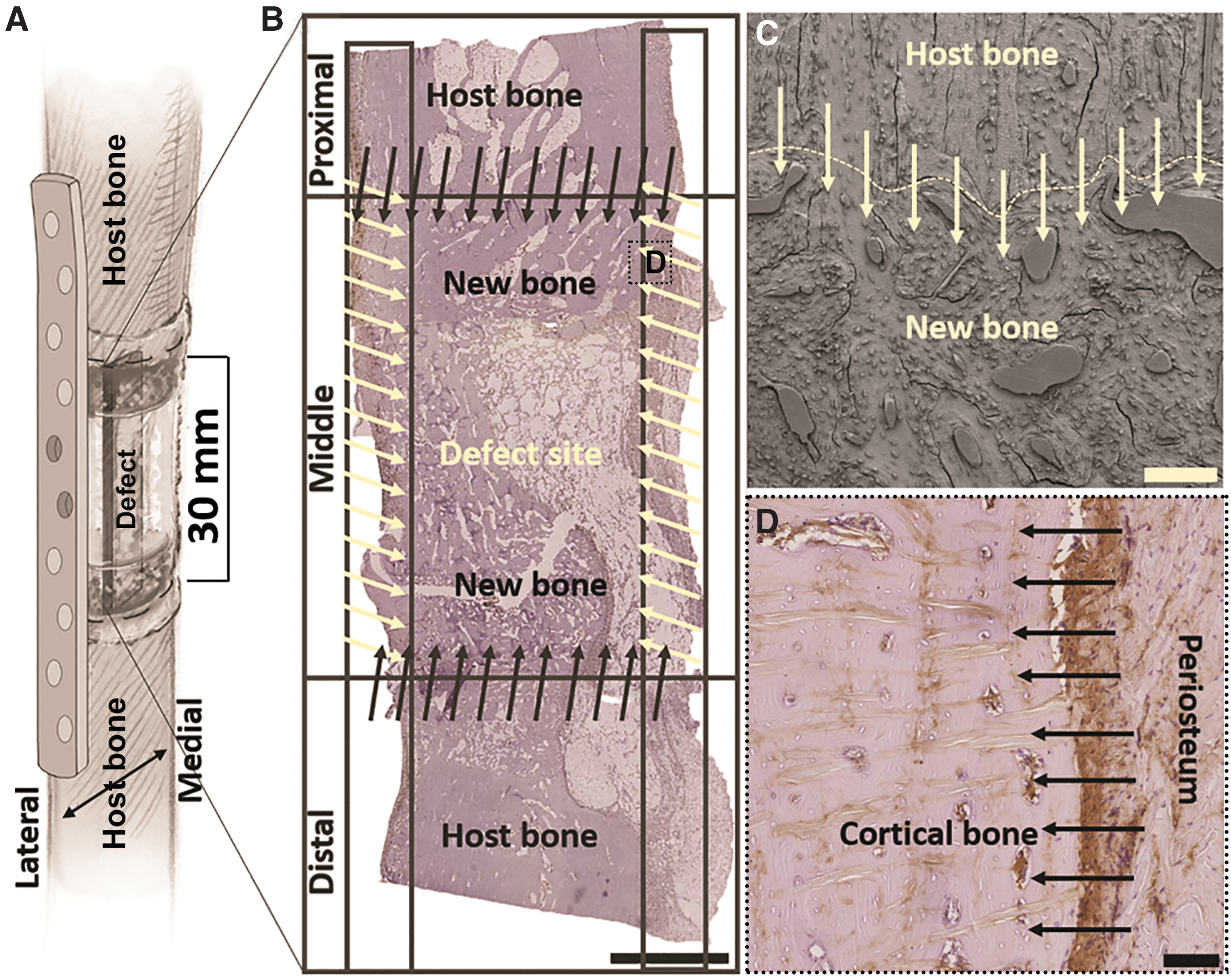
Evaluations such as the inclusion of the levels of surrounding tissue involvement in regulating the newly acquired vasculature for promoting osteogenic cell migration to the defect site, the extent of cortical and trabecular bone remodeling, and the contribution of the distal and proximal host bone in repairing critical-sized bone defects to its preinjury state are scarce.

Although most studies related to bone research have been employing the use of histological and immunohistochemical methods to evaluate bone formation and remodeling, a number of histological evaluations are still based on subjective descriptions and calculations of histological and immunohistochemical staining distributions. However, assumptions about shape, size, cell distribution, and postulations of cell and tissue ratios and densities are the typical sources of bias in semiquantitative and quantitative microscopic image analysis.²⁵

Over the past decade, considerable importance has been given to the use of semiquantitative and quantitative methods to evaluate bone responses to TECs through histological and immunohistochemical image evaluation of overall bone tissue formation, as well as the assessment of ECM-related proteins, inflammatory cells, calcium content, and vascularization.^26–34 Recent developments in quantitative analysis have also been attained with the use of the ImageJ platform^26,35–39 through the implementation and customization of macros and plugins.

Our group²⁸ has previously histomorphometrically evaluated digitized images of entire large bone defect samples based on manual and automated image segmentation modes, using two well-established systems, the Osteomeasure (Osteometrics, Atlanta, GA) and Aperio Image Scope (Leica Biosystems, ScanScope v. 12.3). Despite the ability to quantify features of interest based on measurements of lengths, perimeters, and areas, software programs such as the Osteomeasure system, Aperio Image Scope, Easy Image Measurement 2000, and the Microvid™ image analysis systems are based on a predefined range of color segmentation thresholds, have high variability with respect to the quantification methods, and have been regarded as time-consuming and labor intensive.^27,28,34

Although most image analysis software programs only require image input, image-processing tools including automated image segmentation usability is limited.⁴⁰ Such features are usually obtained by machine learning as described by Arganda-Carreras et al.⁴¹ and Visiofarm,^27,42,43 and with software platforms that provide image-processing tools such as MATLAB (Mathworks, Natick, MA).^44,45

MATLAB is a user-friendly, high-performance matrix-based programming platform designed for engineers and scientists. In the tissue engineering community, MATLAB is also used as an image analysis platform to perform bone histomorphometry.^{36,37,44,46–49} However, the MATLAB approaches employed were used to quantify histological tissue features such as percentage of bone formation, remaining graft material, soft tissue, void areas, and gray scale radiographic images to quantify the degree of bone mineralization. Moreover, none of the developed algorithms offered an automated histomorphometric analysis of immunohistochemically stained sections that would enhance the throughput of large image file data set analysis in an efficient and manageable workflow.

Specific quantification methods are needed to further explore the representative and quantitative structure–function interactions in such a highly hierarchically structured TECs. Here we propose and investigate an in-house written MATLAB algorithm for reviewing large digitized immunohistochemically stained images (∼37265 × 38413 pixels; 4 GB) data sets. The image-processing algorithm is configured to segment, display, and select and quantify regions of interest (ROIs) of a whole slide digital image, enabling the user to analyze the image in <3 min.

Materials and Methods

To evaluate the efficacy of the MATLAB algorithm, it was applied on a broad spectrum of image analysis problems, including: (1)

Sample size and image file size. To investigate the MATLAB algorithm potential and effectiveness we endeavored to test different sample sizes, such as the critical-sized bone defects composed of samples measuring ≥2 × 2 cm and image files (Study 1); abdominal and vaginal hernia defects measuring ≥1 × 3 cm (Study 2); and breast scaffold defect model with samples measuring ≥1 × 4 cm (Study 3). The objective was to evaluate not only on small size image files (≤500 MB), which does not require much time for the algorithm to upload/read the image, but also using larger image files (≥500 MB), which can take longer times to read and process quantification.

(2)

Nonstandardized harvesting sample. Occasionally when harvesting specimen, it is not possible to harvest samples appropriately. Sometimes the material implanted is completely degraded or have moved to make harvesting challenging to standardize. Such samples can have different anatomical sizes and quantification of those different groups cannot be compared equally as the size of the images will be different. The algorithms' ability to choose the size of the ROIs to be analyzed can make the quantification standardized in case of nonstandardized harvesting.

(3)

Diverse immunohistochemical protein markers. One of the major issues hindering the utilization of quantitative analysis of immunohistochemically stained tissue sections is attaining unwanted unspecific protein binding, which results in additional stain background and inherently additional inclusion of false-positive stained areas within the final pixel segmentation quantification. Tissue folds can also be mistaken as positive stained areas.

Study 1

The sample harvesting of this study was not standardized; hence, samples anatomically differ in size. Sample dimension cohort included samples of 1 × 2 cm, 1 × 3 cm, and 2 × 3 cm (W × H). Histological paraffin sections of six parous ewes were sourced from a previous study (Queensland University of Technology Animal Ethics Approval 1800000002).

Two different treatment groups, each containing samples with 3D printed medical grade polycaprolactone (mPCL) scaffolds enriched with platelet-rich plasma in the vagina (20 × 20 mm) and anterior abdominal wall (30 × 30 mm) (group I, n = 2 animals, 4 samples each animal) and samples with the same size light-weight polypropylene mesh scaffold implanted in the vagina and abdominal wall (group II, n = 2 animals, 4 samples each animal) of the sheep. Explanted grafts were retrieved at 3 months (n = 8) and the remainder at 6 months (n = 8). Immunohistochemical evaluation was assessed by von Willebrand factor (vWF, n = 16) and collagen type I (COL I, n = 16). Histological sample preparation and immunohistochemistry staining was performed as described previously.⁶

Study 2

The stained slide sections suffered from nonspecific stain binding. Histological paraffin sections of five pigs were sourced from a previous study (Queensland University of Technology Animal Ethics Approval 1500000613).

Sample size cohort included samples of ≥1 × 4 cm (W × H). A 100 mL tear drop 3D printed breast mPCL scaffolds were implanted in three submuscular pocket defects. Each animal received five different treatments. The five treatment groups, each containing samples with the 3D printed mPCL scaffolds were evaluated in this study: group I (9 samples analyzed), mPCL scaffolds only; group II (10 samples analyzed), mPCL scaffolds were combined with immediate fat graft; group III (10 samples analyzed), mPCL scaffolds were enriched with PRP; group IV (11 samples analyzed), mPCL scaffolds were combined with delayed fat graft; and group V (8 samples analyzed), mPCL scaffolds were combined with PRP and delayed fat graft. Immunohistochemical evaluation was assessed by vWF (n = 48). Histological sample preparation and immunohistochemistry staining was performed as described previously.⁶

Study 3

The sample cohort composed of critical-sized bone defect samples (>2 × 2 cm). Histological paraffin sections of sheep tibiae collected from eight Merino sheep were sourced from a previous study (Queensland University of Technology Animal Ethics Approval No. 0900000425).

Two different treatment groups, each containing samples with a critical-sized 3 cm tibial defect, were evaluated in this study: group I (n = 4; 3 samples each animal—proximal, middle, and distal), the microfiber membrane scaffold was combined with functionalized alginate hydrogel; and group II (n = 4; 3 samples each animal—proximal, middle, and distal), functionalized alginate hydrogel combined with recombinant human bone morphogenic protein 2 (rhBMP-2). Histological assessment was performed on paraffin sections stained with vWF (n = 24). Histological sample preparation and immunohistochemistry staining was performed as described previously.⁶

Experiment—Image Analysis

Images of studies 1 and 2 were acquired using a 3DHistech Scan II Brightfield slide scanner (3DHistech, Budapest, Hungary) at 20 × objective with a spatial resolution of 0.27 μm. Next, images were exported using Case Viewer 2.2 platform (server-based slide management system) in a 1:16 ratio resolution uncompressed tiled TIFF image. Images of Study 3 were acquired using a Leica SCN 400 slide scanner (Leica Microsystems, Wetzlar, Germany) at 20 × with a spatial resolution of 0.50 μm. Images were extracted from the digital image hub using the extract image region of Aperio Image Scope as a uncompressed TIFF image file in a 1:4 ratio resolution.

A total of 520 ROIs were analyzed for this study with 5 ROIs per sample image. Study 1: 16 vWF whole slide images (80 ROIs) and 16 COL I whole slide images (80 ROIs), Study 2: 48 vWF whole slide images (240 ROIs) and Study 3: 24 vWF whole slide images (120 ROIs). The whole slide images and ROI mages were analyzed using MATLAB and Aperio Image Scope software (v.12.3; Aperio Technologies, Inc., CA).

MATLAB

A flowchart describing a developed MATLAB algorithm is given in Figure 3A. The sequence of steps is described as follows:

FIG. 3.

Overview of the MATLAB sequence of steps flowchart (A). Based on L*a*b* color space, the L*a*b* channels threshold are adjusted (B). After the histogram threshold values fine-tuning, an image segmentation mask is created (C) and settings are saved on the MATLAB workspace. Original RGB image is displayed (D) and the image AOI is defined (E, left image). Zoomed-in AOI is displayed, and ROIs are selected (E, right image). ROIs and respective image masks are then displayed (F). AOI, area of interest; FOI, field of interest; ROI, region of interest. Color images are available online.

(1)

Upload original RGB image and run algorithm and variable initialization.

(2)

Define color threshold (algorithm tuning): the color threshold MATLAB application allows for thresholding color images by manipulating the image color based on the different color spaces. The L*a*b* (L*: lightness; a*: red/green value; and b*: blue/yellow value) color space was selected for tuning the immunohistochemically stained images used in this study (Fig. 3B). The live preview of the image allows the user to continuously check and accurately adjust the selection. Based on the chosen threshold values, a segmentation mask is interposed on the original RGB color image used for tuning the algorithm (Fig. 3C).

(3)

Export threshold values function to MATLAB workspace: after defining the threshold values for lightness (L*), red/green (a*), and blue/yellow (b*), the histogram settings function is exported to the MATLAB workspace.

(4)

Display original RGB image: zoom into the image and identify the image area of interest (AOI) (Fig. 3D).

(5)

Define the AOI where the quantification will be performed: using the displayed RGB image, draw rectangle to zoom into the desired field of interest. Define the number of ROIs and select ROIs within the AOI (Fig. 3E).

(6)

If ROI selection is satisfactory press ENTER. ROIs and respective image masks are then displayed according to the threshold values selected in step 2 (Fig. 3F). If ROI selection is unsatisfactory repeat step 2.

(7)

Pixel count for each variable of interest (vWF, Col I, blood vessels) is performed on the segmented ROIs (masks) from step 5 and results are displayed and exported as an Excel file.

The size of the five ROIs used for the image analysis quantification of studies 1 and 3 were 1000 (H) × 1000 (W) pixel, whereas for Study 2 the ROIs were 2000 (H) × 2000 (W) pixel. All ROIs created with MATLAB were saved individually as a TIF file.

To set the correct threshold values, it should be noted that the tuning of the image needs to be performed for each set of images (studies 1, 2 and 3) and for each IHC marker (COL I and vWF). Failure to do so will result in default thresholds being used, which may not represent the correct pixel segmentation.

The algorithm segments the positive immunohistochemically stained image pixels in each ROI according to the L*a*b* (channels 1, 2, and 3) thresholds. The segmented ROI images are then quantified relatively to the ROI total number of columns and rows.

The threshold values used for the vWF staining were based on the histogram settings function exported as follows: for channel 1 (L*) min = 2.632 and max = 37.233; for channel 2 (a*): min = −14.641 and max = 79.188; and for channel 3 (b*) min = −0.489; and max = 31.955. For COL I it was as follows: for channel 1 (L*) min = 45.261 and max = 83.505; for channel 2 (a*) min = 1.349 and max = 8.982; and for channel 3 (b*) min = −107.860 and max = 33.215.

Blood vessel pixel total number was performed by counting the pixels selected by the L*a*b* thresholds. Percentage (%) of blood vessel pixel number was calculated as follows: 100* × blood vessels pixel number within the ROI divided by the ROI size (total number of rows by the total number of columns measured in pixels). The same calculation parameters were applied to the COL I variable. Void areas were selected as grayscale image (0–255). The threshold value of 252 was selected for areas within each ROI where there was no tissue sample, or empty void spaces.

Aperio image scope

All the ROIs created with MATLAB were also analyzed using the Aperio Image Scope Positive Pixel Count (PPC) algorithm.

The Aperio PPC algorithm is an image analysis algorithm that performs whole slide digital image analysis, based on the hue, saturation, and intensity (HSI) color space. Although the Aperio PPC algorithm has input parameters settings selected by default, these parameters can be adjusted to best suit histological staining color selection.

By adjusting the intensity of a hue value, the Aperio PPC algorithm defines a specific stain hue value and subsequently sets this selection as a referential pixel. Hue saturation and hue intensity threshold are then adjusted. All pixels within that HSI range will be selected. Within these parameters adjusted, the Aperio PPC algorithm measures three categories of staining: strong positive staining (red color), medium positive staining (orange color), weak positive staining (yellow color), and negative staining (blue color). Aperio Image Scope color space and the Aperio PPC algorithm setting parameters are described in full in ref.²⁸

The Aperio PPC algorithm parameters were adjusted for each image to best identify the pixel selection related to the COL I immunohistochemical staining identified as weak positive and to the background identified as weak positive stain, and to the vWF immunohistochemical staining identified as strong positive and to the background identified as medium positive stain. Using the ROIs created and saved with MATLAB, the following settings were applied:

(1)

COL I immunohistochemically stained samples in Study 1: hue value of 0.1 (brown), hue width of 0.4, and color saturation of 0.04. The threshold of the intensity of the weak positive stain (Iwp (High)) was adjusted between 170 and 210 to eliminate unspecific and background staining.

(2)

vWF immunohistochemically stained samples in Study 1: hue value of 0.1 (brown), hue width of 0.5, and color saturation of 0.04. The threshold of the intensity of the medium positive stain (Ip(Low) = Isp(High)) was adjusted between 86 and 101 to eliminate unspecific and background staining.

(3)

The vWF immunohistochemically stained samples of Study 2: hue value of 0.1 (brown), hue width of 0.5, and color saturation of 0.04. A threshold within 63–85 was applied to the intensity of the medium positive stain to eliminate unspecific and background staining.

(4)

The vWF stained samples of Study 3: hue value of 0.1 (brown), hue width of 0.5, and color saturation of 0.04. A threshold within 35–102 was applied to the intensity of the strong positive stain to eliminate unspecific and background staining.

Based on the threshold intensity of COL I and vWF for each ROI, the number of pixels selected within the selected threshold range was obtained. A percentage of the total stained area in each ROI was calculated based on the total area pixel of that ROI. The average of the five ROIs was then calculated to plot the graphs.

Statistical analysis

For each sample, a sum of the quantified percentage area stained for the five ROIs was obtained. Statistical analysis was obtained with GraphPad Prism version 7.03 and Microsoft Excel. Agreement between the image analysis results were evaluated by Pearson correlation coefficient (R²) and 95% confidence intervals (CIs). A correlation coefficient of 1 or −1 corresponded to a perfect linear correlation between two measurements. A 0-value corresponded to no correlation between measurements. Intersystem analysis was performed between Aperio Image Scope and MATLAB image analysis methods according to Bland–Altman using the 95% limits of agreement (LOA) as the mean of the two paired measurements, minus and plus 1.96 standard deviations.⁵⁰ t-test was used to compare image analysis method (Aperio PPC algorithm vs. MATLAB) measurements without treatment distinction. Significance was defined as p < 0.05.

Results

The proposed MATLAB algorithm was tested on three different image data sets to demonstrate the efficacy of the proposed MATLAB algorithm on a broad spectrum of biomedical image analysis problems. In Study 1, the sample harvesting was not standardized, hence samples differed in anatomical size; in Study 2, the stained slide sections suffered from nonspecific stain binding; and in Study 3, the sample cohort composed of critical-sized bone defect samples. A total of 520 ROI images were analyzed using the Aperio PPC and MATLAB algorithms. The histomorphometric results of studies 1, 2, and 3 obtained with each algorithm were compared and investigated.

The intersystem comparison between the Aperio Image Scope and the MATLAB histomorphometric evaluation of the ROIs % area stained of Study 1 for COL I at 3- and 6-month time point (Fig. 4A, B) presented a high and positive correlation, R² = 0.99. The histomorphometric measurements were in excellent agreement with most of the paired measurements lying within the 95% LOA (Fig. 4C). Similarly, the Pearson's correlation of the histomorphometric evaluation of Study 1 vWF immunohistochemical stain at 3 and 6 months (Fig. 4D, E) was also high and positive (R² = 0.99). The vWF Bland–Altman analysis also indicated a strong agreement between the vWF PPC Aperio Image Scope and MATLAB measurements, with all the paired measurements lying within the 95% LOA (Fig. 4F).

FIG. 4.

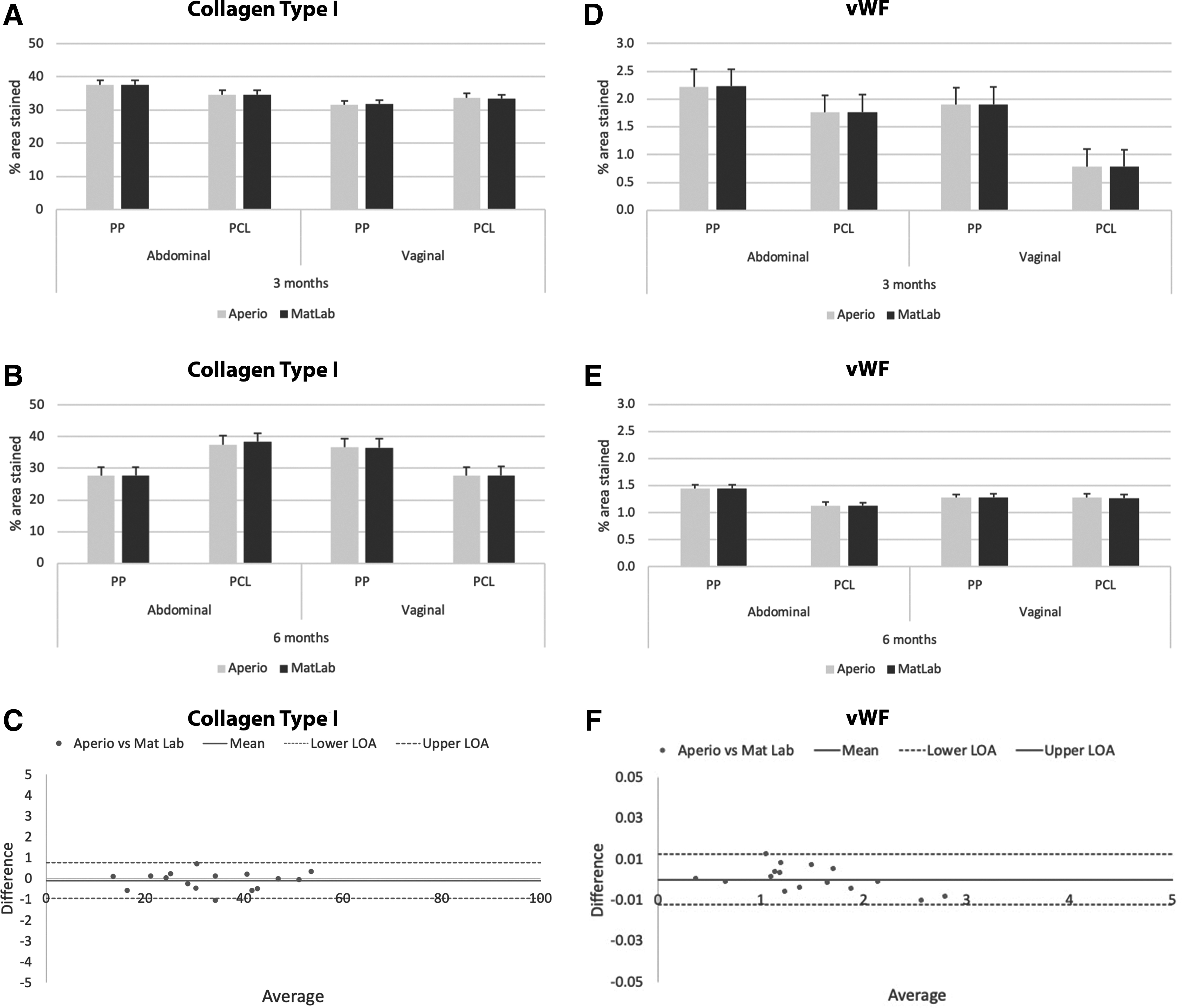
Study 1 intersystem comparison between Aperio Image Scope and MATLAB histomorphometric evaluation for COL I % area stained (A–C) and vWF (D–F) immunohistochemical stain. COL I measurements at 3 (A) and 6 (B) months using Aperio Image Scope and MATLAB (t-test, p = 0.9955, R² = 0.99); (C) COL I Bland–Altman plot comparing Aperio Image Scope and MATLAB measurements; vWF measurements at 3 (D) and 6 (E) months using Aperio Image Scope and MATLAB (t-test, p = 0.9842, R² = 0.99); (F) vWF Bland–Altman plot comparing Aperio Image Scope and MATLAB measurements (LOA, 1.96 SD). COL I, collagen type I; LOA, limit of agreement; SD, standard deviation; vWF, von Willebrand factor.

The descriptive statistical analyses of COL I and vWF obtained with the Aperio PPC algorithm did not differ from the MATLAB algorithm, which was further confirmed by calculated p-values of 0.9955 and 0.9994, respectively (Supplementary Table S1).

The intersystem comparison between the Aperio Image Scope and MATLAB histomorphometric evaluation of Study 2 for vWF immunohistochemical stain (Fig. 5A) were in excellent agreement (R² = 0.99). Most of the paired measurements were within 95% LOA as depicted by the Bland–Altman analysis (Fig. 5B), except for one pairwise of measurement, where the MATLAB histomorphometric measurement was higher than the measurements attained with the Aperio PPC algorithm, suggesting a slight variability between the measurements. However, when analyzing the vWF immunohistochemical stain descriptive statistical results, all the measurements obtained with the Aperio PPC and MATLAB algorithms were within the 95% CI, which was further confirmed by calculated p-value (p = 0.9920) (Supplementary Table S1, Study 2).

FIG. 5.

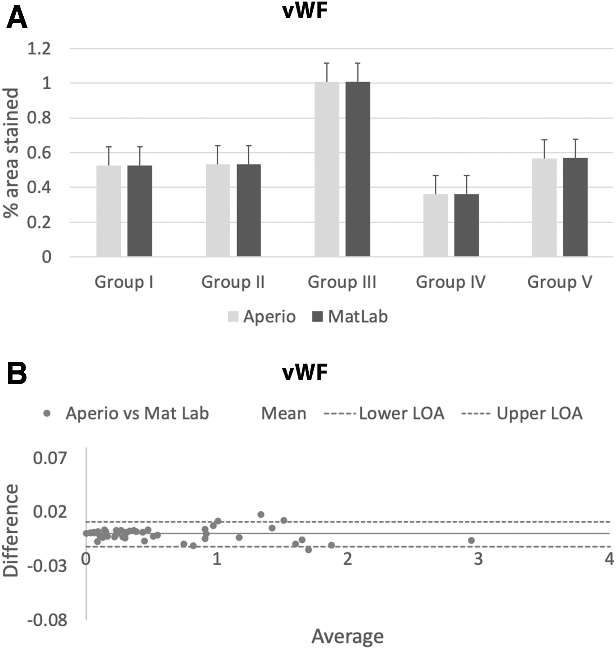
Study 2 intersystem comparison between Aperio Image Scope and MATLAB histomorphometric evaluation for vWF immunohistochemical stain % area stained. (A) vWF measurements using Aperio Image Scope and MATLAB (t-test, p = 0.9920, R² = 0.99); (B) vWF Bland–Altman plot comparing Aperio Image Scope and MATLAB measurements (LOA, 1.96 SD).

The intersystem comparison between Aperio Image Scope and MATLAB histomorphometric evaluation of Study 3 for vWF immunohistochemical staining showed the same measurements trends using the Aperio PPC and MATLAB algorithms (Fig. 6A). The measurements were in excellent agreement (R² = 0.99) and no significant difference were found within the paired measurements (p = 0.9615). However, there was one paired of measurements outside the 95% LOA as depicted by the Bland–Altman analysis in Figure 6B. The vWF histomorphometric measurements obtained with the MATLAB algorithm were slightly higher than the measurements obtained with the Aperio PPC algorithm; however, no significant differences were found between the measurements (p = 0.9874). All measurements obtained with the Aperio PPC and MATLAB algorithms were within the 95% CI (Supplementary Table S1, Study 3).

FIG. 6.

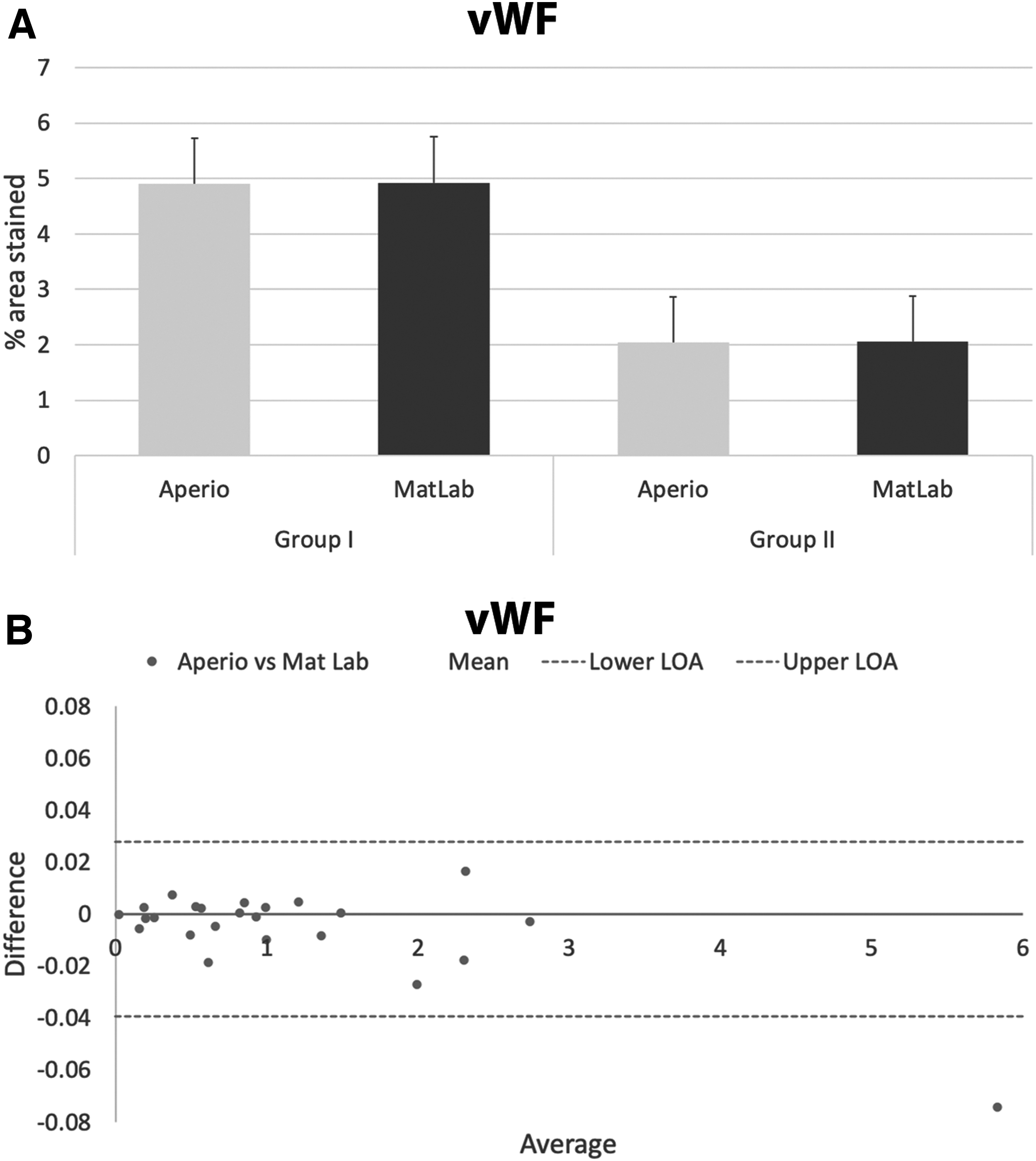
Study 3 intersystem comparison between Aperio Image Scope and MATLAB histomorphometric evaluation for vWF immunohistochemical stain % area stained. (A) vWF measurements using Aperio Image Scope and MATLAB (t-test, p = 0.9615, R² = 0.99); (B) vWF Bland–Altman plot comparing Aperio Image Scope and MATLAB measurements (LOA, 1.96 SD).

Figure 7 illustrates an overview and comparison of the original ROI images of COL I and vWF staining (Fig. 7A, D), and the ROI images mask selection obtained with the MATLAB (Fig. 7B, E) and Aperio PPC (Fig. 7C, F) algorithms for COL I and vWF staining, respectively.

FIG. 7.

Overview and comparison of the COL I and (A–C) and vWF (D–F) immunohistochemical staining segmentation using MATLAB (B, E) and Aperio PPC algorithms (C, F) of Study 1. (A, D) The original ROIs obtained with the MATLAB algorithm. (B, E) The ROI image masks of the COL I and vWF pixel segmentation obtained with the MATLAB algorithm. The light brown color (B) illustrates the positive COL I staining selection and the strong brown color (E) illustrates the positive vWF staining selection. (C, F) The ROI image masks of the COL I and vWF pixel segmentation obtained with the Aperio PPC algorithm. Yellow color (C) depicts the weak positive staining selection of the COL I staining. The orange color depicts the medium positive staining selection of the COL I and vWF in images (C, F). The red color (F) depicts the strong positive for vWF. Single black arrows in images (A–C) indicate staining color variability; red arrow in images (D–F) indicates a tissue section fold resultant from slide section preparation and double black arrows indicate staining background. Scale bars: 100 μm. Color images are available online.

Overall, the intersystem comparison of the MATLAB and Aperio PPC segmentation algorithms for the COL I and vWF histomorphometric did not differ as depicted by the mask images. However, Aperio PCC algorithm selection was slightly less selective in areas where there was color staining variability (Fig. 7C single black arrow), histological slide preparation artifacts (tissue folds) (Fig. 7F red arrows), and unspecific chromogenic binding (staining background) (Fig. 7F double black arrows). These issues did not interfere with the MATLAB segmentation process.

Discussion

While appraising quantitative data, histomorphometric analysis of digitized images can be compromised and biased by a variety of inherent specimen factors and intrinsic variation in histological and immunohistochemical staining protocols as well as by image analysis statistical assessment. Aspects inherent to sample specimens include the specimen sample size and the anatomical variation within animals. Intrinsic elements related to histological and immunohistochemical staining protocols include stain color variability and the presence of unspecific staining binding.

Factors affecting image analysis statistical assessment include microscope magnification, scale factors, image file size, color threshold, and the lack of appropriate statistical methods, including the absence of appropriate histomorphometric approaches that accurately represents anatomical sample section planes, histological sections numbers, and a minimum number of ROIs that accurately represent the entire defect sample analyzed.^28,51

Manual microscopy imaging is usually limited to the analysis of an ROI at a specific magnification within a limited tissue area, at a time. In parallel, most histological analyses are focused on a single structure or a type of tissue under the assumption that all features within an entire sample section would appear in a regular and cyclic spatial arrangement. Wagermaier et al.,²² reviewing scanning X-ray scattering methods for understanding the hierarchy and functions of bone, state that distinct levels of hierarchy from nanometer to the macroscopic scale can be observed during bone repair. Thus, image analyses are directly associated with the magnification used for acquiring the histological image and the image pixel array representing the image.

The ability of MATLAB to zoom into an AOI within an entire sample section makes this feature valuable. Decreased zoom displays less cellular details while providing a greater macroscopic histological overview, whereas increased zoom allows for greater observation of cellular details. When analyzing small structures, such as blood vessels, proper sample visualization is a requisite for distinguishing vascular basement membrane from the marrow tissue and ground substance of the connective tissue surrounding the tissue section samples.

Another advantage of the presented MATLAB approach includes the ability to define the size and the number of ROIs to be used. Key aspects that need to be considered in the validation of immunohistochemical staining include outdated nominal and sometimes ordinal data evaluations obtained through descriptive and semiquantitative methods, which rarely promote reproducibility.⁵² When animal sample harvesting is not standardized, it is difficult to compare treatment groups as there is anatomical tissue size disparity within the sample cohort. In defining the size of the ROI, the user is standardizing the quantification. Yet, this procedure will ensure that all treatments will be analyzed automatically and in the same manner.

The ability to define and choose the number of ROIs must be carefully pondered. Gerstenfeld et al.,⁵¹ reviewing the specific technical considerations for the application of histomorphometric methods to the study of bone repair, compared and developed reference values by measuring transverse callus fracture sections using ROIs at 100 μm apart. By comparing the mean values and 95% confidence intervals (CI) of the histomorphometric data, the authors concluded that the highest statistical variability was obtained when using less than five ROIs per section. Despite increasing the distance between the ROIs to 500 μm apart, the results still fell within the 95% CI. These findings corroborate our descriptive statistical analysis results. Although Study 1 presented a wider CI within the samples analyzed (less number of samples), the mean values obtained with the Aperio PPC and MATLAB algorithms using five ROIs fell within the 95% CI.

Whereas X-ray scattering approaches for correlating anatomy with function have improved and become more accessible, precise, accurate, and faster immunohistochemical evaluation methods are still stagnant. Although a few image analysis systems quantify large image files, these systems are based on the manual selection of tissue features, drawing of equidistant lines, and the use of superimposed grids containing boundary points to obtain measures of tissue regeneration.^21,28,53,54 These approaches require fine hand motor coordination for selecting specific stained areas as immunohistochemical assays stain specific portions of tissues or specific cells, making this procedure tiring and time-consuming, especially considering the size of large tissue sections.

In addition, most of these image analysis systems do not retain the selected measurements with respective image files, thereby requiring reloading of the images and their reassessment.²⁸ The capacity of our MATLAB algorithm to automatically select stained areas of specific protein markers, to save the ROIs and respective mask images, and to reanalyze the image files without the need of reloading the full image, saves the user's time.

The correlation between immunohistochemical outcomes to detect protein markers expressing specific cellular phenotypes to predict the likelihood of a response requires proper protein specific binding distinguishability from unspecific chromogenic binding. One of the major factors hindering the utilization of quantitative analysis of immunohistochemically stained tissue sections is the paucity of standardized immunohistochemical protocols for determining the specificity of antibodies. Immunohistochemistry relies upon the antibody–antigen binding specificity within a histological tissue section, and the following visualization of these bound antibodies.⁵⁵ There is an array of variables to consider, such as the diaminobenzidine (DAB) chromogenic stain detection, while preserving the sensitivity and specificity of the antibody.

The DAB chromogenic immunohistochemical stain relies on the development of a brown color at the site of enzymatic activity.⁵⁶ The protracted time of chromogen application results in unwanted unspecific protein binding. DAB incubation must be stringently controlled to achieve reproducible staining intensity.⁵⁷ This issue was observed with the vWF results obtained with the Aperio image analysis system. The threshold of the Aperio PPC algorithm had to be adjusted to avoid areas of unspecific protein binding, such as the ground substance within the connective tissue and bone morrow cavities of the vWF results of Study 2 and Study 3, respectively.

The possible reason for this issue may rely on the color space vector distance between two colors used. The Aperio PPC algorithm works with HSI color space, whereas MATLAB works with L*a*b* color space. Bueno et al.,⁵⁸ analyzing different color models for microscopic image processing based on the distance of two colors, proposed that the vector distance of the HSI color space differentiates well between two colors; however, the L*a*b* color space distinguishability of the original image color is of superior quality. Similarly, Wang et al.,⁵⁹ while proposing a color quantification algorithm based on the L*a*b* color space for evaluation of stained tissues, stated that the rationale behind the consistency of the L*a*b color space quantification relies on the perceptual similarity to human perception of color change.

One of the advantages of the presented MATLAB algorithm is the ability to adjust the image thresholding selection based on the live L*a*b* channels histogram preview. The Aperio PPC algorithm does not provide live histogram channels preview, instead, the thresholding settings is based on a specific HSI color threshold value range. Consequently, segmentation process is more challenging and time-consuming as it is very difficult to find a specific threshold value that can be used for input images containing histological artifacts such as uneven tissue section, tissue folds, and unspecific staining background. These areas are detected and mistaken as positive stained areas, thus affecting final histomorphometric quantifications.

When using very large image files (≥4 GB), most image analysis software packages become unresponsive, or owing to proprietary file format restrictions and file size limitations (defined number of image pixel dimension that the software can work with), do not display or allow zooming out to a smaller scale than the original saved image file. In addition, Aperio Image Scope does not provide live threshold preview selection, the user must manually select color threshold, apply to the image, and visualize. If threshold selection is not satisfactory, the user needs to repeat the threshold selection several times to achieve a satisfactory pixel color selection. On the contrary, machine learning segmentation approaches are based on a training set of features, where pixels are classified as belonging to a specific tissue feature, which considering the dynamic variability and heterogeneous distribution of cells within a remodeling tissue site, are likely to not present the same pattern and features within an entire tissue sample.

Quantitative evaluation of histologically or immunohistochemically stained tissue sections, usually involves selecting ROIs and excluding false-positive stained areas, including the exclusion of tissue folds and unspecific staining background. Bouzin et al.⁶⁰ assessing the influence of the presence and absence of tissue folds using automated image analysis reported that quantification was biased, however not affected by the presence of tissue folds, as long as the percentage area of tissue fold is <5%. Whether quantification is affected or not, the exclusion of background staining and tissue folds remains a challenging and time-consuming task, and the presented MATLAB algorithm overcomes this issue.

The lack of standardization of sample harvesting, preparation of the histological slide section, variability in staining protocols, interobserver subjectivity, variability and complexity in quantification methods, and the lack of well-defined quantifiable parameters to evaluate immunohistochemical results makes this MATLAB algorithm a potential approach to expedite and promote objective and reproducible quantitative assessments of large tissue sections (37265 × 38413 pixels; 4 GB).

Features of the proposed MATLAB approach include the ability to segment large image files, automated identification of immunohistochemically stained sections based on a lively color space tuning; selection of AOI and magnification of this area; definition of number and size of the ROIs to be analyzed; ability to reanalyze the image without the need of reloading the full image and the capability of displaying and exporting the results of all ROIs as an Excel file format in an efficient and manageable workflow.

Footnotes

Acknowledgments

The authors acknowledge distinguished professor Dietmar W. Hutmacher for his guidance, advice, and feedback on this article. The authors gratefully acknowledge Jan Henkel and Jan Janzekovic for providing the sheep and pig specimens used in this study. The authors also thank the Histology Facility Central Analytical Research Facility (CARF), and Institute of Health and Biomedical Innovation (IHBI) at Queensland University of Technology (QUT) for providing general facility support.

Disclosure Statement

No competing financial interests exist.

Funding Information

Financial support for this project was provided by the Australian Research Council (ARC) Industrial Transformation Training Centre in Additive Biomanufacturing (IC 160100026) and by the ARC Industrial Transformation Training Centre for Multiscale 3D Imaging, Modelling, and Manufacturing (IC 180100008).

Supplementary Material

References

Gugala

, and Gogolewski

Regeneration of segmental diaphyseal defects in sheep tibiae using resorbable polymeric membranes: a preliminary study. J Orthop Trauma, 13, 187, 1999.

Schemitsch

E.H.

Size matters: defining critical in bone defect size!. J Orthop Trauma, 31, S20, 2017.

Berner

, Boerckel

J.D.

, Saifzadeh

, et al. Biomimetic tubular nanofiber mesh and platelet rich plasma-mediated delivery of BMP-7 for large bone defect regeneration. Cell Tissue Res, 347, 603, 2012.

Berner

, Henkel

, Woodruff

M.A.

, et al. Delayed minimally invasive injection of allogenic bone marrow stromal cell sheets regenerates large bone defects in an ovine preclinical animal model. Stem Cells Transl Med, 4, 503, 2015.

Sparks

D.S.

, Savi

F.M.

, Saifzadeh

, et al. Convergence of scaffold-guided bone reconstruction and surgical vascularization strategies—a quest for regenerative matching axial vascularization. Front Bioeng Biotechnol, 7, 448, 2020.

Sparks

D.S.

, Saifzadeh

, Savi

F.M.

, et al. A preclinical large-animal model for the assessment of critical-size load-bearing bone defect reconstruction. Nat Protoc, 15, 877, 2020.

Kirby

, White

, Steck

, et al. Microparticles for sustained growth factor delivery in the regeneration of critically-sized segmental tibial bone defects. Materials (Basel), 9, 259, 2016.

Reichert

J.C.

, Cipitria

, Epari

D.R.

, et al. A tissue engineering solution for segmental defect regeneration in load-bearing long bones. Sci Transl Med, 4, 141ra93, 2012.

Berner

, Reichert

J.C.

, Woodruff

M.A.

, et al. Autologous vs. allogenic mesenchymal progenitor cells for the reconstruction of critical sized segmental tibial bone defects in aged sheep. Acta Biomater, 9, 7874, 2013.

10.

Cipitria

, Reichert

J.C.

, Epari

D.R.

, et al. Polycaprolactone scaffold and reduced rhBMP-7 dose for the regeneration of critical-sized defects in sheep tibiae. Biomaterials, 34, 9960, 2013.

11.

Reichert

J.C.

, Wullschleger

M.E.

, Cipitria

, et al. Custom-made composite scaffolds for segmental defect repair in long bones. Int Orthop, 35, 1229, 2011.

12.

Reichert

J.C.

, Woodruff

M.A.

, Friis

, et al. Ovine bone- and marrow-derived progenitor cells and their potential for scaffold-based bone tissue engineering applications in vitro and in vivo. J Tissue Eng Regen Med, 4, 565, 2010.

13.

Cipitria

, Wagermaier

, Zaslansky

, et al. BMP delivery complements the guiding effect of scaffold architecture without altering bone microstructure in critical-sized long bone defects: a multiscale analysis. Acta Biomater, 23, 282, 2015.

14.

Cipitria

, Lange

, Schell

, et al. Porous scaffold architecture guides tissue formation. J Bone Miner Res, 27, 1275, 2012.

15.

Kerschnitzki

, Kollmannsberger

, Burghammer

, et al. Architecture of the osteocyte network correlates with bone material quality. J Bone Miner Res, 28, 1837, 2013.

16.

Berner

, Henkel

, Woodruff

M.A.

, et al. Scaffold-cell bone engineering in a validated preclinical animal model: precursors vs differentiated cell source. J Tissue Eng Regen Med, 11, 2081, 2017.

17.

Donnelly

Methods for assessing bone quality: a review. Clin Orthop Relat Res, 469, 2128, 2011.

18.

Paris

, Götz

, Hettrich

, et al. Scaffold curvature-mediated novel biomineralization process originates a continuous soft tissue-to-bone interface. Acta Biomater, 60, 64, 2017.

19.

Y.H.

, and Martin

K.L.

Handbook of Histology Methods for Bone and Cartilage. Totowa, NJ: Humana Press, 2003.

20.

Rentsch

, Schneiders

, Manthey

, et al. Comprehensive histological evaluation of bone implants. Biomatter, 4, e27993, 2014.

21.

Dalle Carbonare

, Valenti

M.T.

, Bertoldo

, et al. Bone microarchitecture evaluated by histomorphometry. Micron, 36, 609, 2005.

22.

Wagermaier,. W., Gourrier, A., Aichmayer, B., et al. Understanding hierarchy and functions of bone using scanning x-ray scattering methods. In: Bréchet

, ed. Materials Design Inspired by Nature: Function Through Inner Architecture. Cambridge, United Kingdom: RSC Publishing, 2013, pp. 46–73.

23.

Kulak

.a.M., and Dempster

D.W

. Bone histomorphometry: a concise review for endocrinologists and clinicians. Arq Bras Endocrinol Metabol, 54, 87, 2010.

24.

Safadi,. F.F., Barbe, M.F., Abdelmagid, S.M., et al. Bone structure, development and bone biology. In: Khurana

J.S.

, ed. Bone Pathology. Totowa, NJ: Humana Press, 2009, pp. 1–50.

25.

Mühlfeld

, Nyengaard

J.R.

, and Mayhew

T.M.

A review of state-of-the-art stereology for better quantitative 3D morphology in cardiac research. Cardiovasc Pathol, 19, 65, 2010.

26.

van't Hof

R.J.

, Rose

, Bassonga

, et al. Open source software for semi-automated histomorphometry of bone resorption and formation parameters. Bone, 99, 69, 2017.

27.

Zhang

, Chang

, Beck

.a., et al. Analysis of new bone, cartilage, and fibrosis tissue in healing murine allografts using whole slide imaging and a new automated histomorphometric algorithm. Bone Res, 4, 15037, 2016.

28.

Medeiros Savi

, Lawrence

, Hutmacher

D.W.

, et al. Histomorphometric analysis of critical-sized bone defects using Osteomeasure and Aperio systems. Tissue Eng Part C Methods, 25, 732, 2019.

29.

Fedchenko

, and Reifenrath

Different approaches for interpretation and reporting of immunohistochemistry analysis results in the bone tissue—a review. Diagn Pathol, 9, 221, 2014.

30.

Lejeune

, Jaén

, Pons

, et al. Quantification of diverse subcellular immunohistochemical markers with clinicobiological relevancies: validation of a new computer-assisted image analysis procedure. J Anat, 212, 868, 2008.

31.

Tayrac

, Alves

, and Thérin

Collagen-coated vs noncoated low-weight polypropylene meshes in a sheep model for vaginal surgery. A pilot study. Int Urogynecol J, 18, 513, 2007.

32.

Goodwin

P.C.

, Johnson

, and Frevert

C.W.

Microscopy, immuno-histochemistry, digital imaging, and quantitative microscopy. In: Treuting

P.M.

, Dintzis

S.M.

, and Montine

K.S.

, eds. Comparative Anatomy and Histology. Contoocook, NH: Elsevier, 2018, pp. 53–66.

33.

Han

, Bhavsar

, Leppik

, et al. Histological scoring method to assess bone healing in critical size bone defect models. Tissue Eng Part C Methods, 24, 272, 2018.

34.

Egan

K.P.

, Brennan

T.A.

, and Pignolo

R.J.

Bone histomorphometry using free and commonly available software. Histopathology, 61, 1168, 2012.

35.

Della Mea

, Baroni

G.L.

, Pilutti

, et al. SlideJ: An ImageJ plugin for automated processing of whole slide images. PLoS One, 12, 1, 2017.

36.

Malhan

, Muelke

, Rosch

, et al. An optimized approach to perform bone histomorphometry. Front Endocrinol (Lausanne), 9, 1, 2018.

37.

Walsh

W.R.

, Oliver

R.A.

, Christou

, et al. Critical size bone defect healing using collagen-calcium phosphate bone graft materials. PLoS One, 12, 1, 2017.

38.

Wen

, Murach

K.A.

, Vechetti

I.J.

, et al. Myo Vision: software for automated high-content analysis of skeletal muscle immunohistochemistry. J Appl Physiol, 124, 40, 2018.

39.

Law

A.M.K.

, Yin

J.X.M.

, Castillo

, et al. Andy's Algorithms: new automated digital image analysis pipelines for FIJI. Sci Rep, 7, 1, 2017.

40.

Ducheyne

Comprehensive Biomaterials. Amsterdam: Elsevier, 2011.

41.

Arganda-Carreras

, Kaynig

, Rueden

, et al. Trainable Weka Segmentation: a machine learning tool for microscopy pixel classification. Bioinformatics, 33, 2424, 2017.

42.

Eriksen

A.C.

, Andersen

J.B.

, Kristensson

, et al. Computer-assisted stereology and automated image analysis for quantification of tumor infiltrating lymphocytes in colon cancer. Diagn Pathol, 12, 1, 2017.

43.

Stålhammar

, Fuentes Martinez

, Lippert

, et al. Digital image analysis outperforms manual biomarker assessment in breast cancer. Mod Pathol, 29, 318, 2016.

44.

Malhotra

, Pelletier

, Oliver

, et al. Platelet-rich plasma and bone defect healing. Tissue Eng Part A, 20, 2614, 2014.

45.

Sompuram

S.R.

, Vani

, Schaedle

A.K.

, et al. Quantitative assessment of immunohistochemistry laboratory performance by measuring analytic response curves and limits of detection. Arch Pathol Lab Med, 142, 851, 2018.

46.

Slyfield

C.R.

, Tkachenko

E.V.

, Wilson

D.L.

, et al. Three-dimensional dynamic bone histomorphometry. J Bone Miner Res, 27, 486, 2012.

47.

Dempster

D.W.

, Brown

J.P.

, Fahrleitner-Pammer

, et al. Effects of long-term denosumab on bone histomorphometry and mineralization in women with postmenopausal osteoporosis. J Clin Endocrinol Metab, 103, 2498, 2018.

48.

Klintström

, Smedby, Ö., Moreno

, et al. Trabecular bone structure parameters from 3D image processing of clinical multi-slice and cone-beam computed tomography data. Skeletal Radiol, 43, 197, 2014.

49.

Hyun Hong

Computer-automated static, dynamic and cellular bone histomorphometry. J Tissue Sci Eng, 05, 1, 2012.

50.

Martin Bland

, and Altman

Statistical methods for assessing agreement between two methods of clinical measurement. Lancet, 327, 307, 1986.

51.

Gerstenfeld

L.C.

, Wronski

T.J.

, Hollinger

J.O.

, et al. Application of histomorphometric methods to the study of bone repair. J Bone Miner Res, 20, 1715, 2005.

52.

Dunstan

R.W.

, Wharton

K.A.

, Quigley

, et al. The use of immunohistochemistry for biomarker assessment-Can it compete with other technologies? Toxicol Pathol, 39, 988, 2011.

53.

Stavropoulos

, Dahlin

, Ruskin

J.D.

, et al. A comparative study of barrier membranes as graft protectors in the treatment of localized bone defects: an experimental study in a canine model. Clin Oral Implants Res, 15, 435, 2004.

54.

Elgali

, Turri

, Xia

, et al. Guided bone regeneration using resorbable membrane and different bone substitutes: early histological and molecular events. Acta Biomater, 29, 409, 2016.

55.

Dagleish

M.P.

, Benavides

, and Chianini

Immunohistochemical diagnosis of infectious diseases of sheep. Small Rumin Res, 92, 19, 2010.

56.

Rimm

D.L.

What brown cannot do for you. Nat Biotechnol, 24, 914, 2006.

57.

Shi

S.R.

, Liu

, and Taylor

C.R.

Standardization of immunohistochemistry for formalin-fixed, paraffin-embedded tissue sections based on the antigen-retrieval technique: from experiments to hypothesis. J Histochem Cytochem, 55, 105, 2007.

58.

Bueno

, González

, Déniz

, et al. Colour model analysis for microscopic image processing. Diagn Pathol, 3, 1, 2008.

59.

Wang

, Shi

, Wang

Y.X.J.

, et al. Color quantification for evaluation of stained tissues. Cytom Part A, 79 A, 311, 2011.

60.

Bouzin

, Saini

M.L.

, Khaing

K.K.

, et al. Digital pathology: elementary, rapid and reliable automated image analysis. Histopathology, 68, 888, 2016.